https://doi.org/10.5194/cp-13-1851-2017 © Author(s) 2017. This work is distributed under the Creative Commons Attribution 3.0 License.
Comparing proxy and model estimates of hydroclimate
variability and change over the Common Era
PAGES Hydro2k Consortium
A full list of authors and their affiliations appears at the end of the paper.
Correspondence:Jason E. Smerdon ([email protected])
Received: 8 March 2017 – Discussion started: 7 April 2017
Revised: 24 August 2017 – Accepted: 11 September 2017 – Published: 20 December 2017
Abstract.Water availability is fundamental to societies and ecosystems, but our understanding of variations in hydrocli-mate (including extreme events, flooding, and decadal pe-riods of drought) is limited because of a paucity of mod-ern instrumental observations that are distributed unevenly across the globe and only span parts of the 20th and 21st centuries. Such data coverage is insufficient for character-izing hydroclimate and its associated dynamics because of its multidecadal to centennial variability and highly regional-ized spatial signature. High-resolution (seasonal to decadal) hydroclimatic proxies that span all or parts of the Common Era (CE) and paleoclimate simulations from climate mod-els are therefore important tools for augmenting our under-standing of hydroclimate variability. In particular, the com-parison of the two sources of information is critical for ad-dressing the uncertainties and limitations of both while en-riching each of their interpretations. We review the princi-pal proxy data available for hydroclimatic reconstructions over the CE and highlight the contemporary understanding of how these proxies are interpreted as hydroclimate indi-cators. We also review the available last-millennium simula-tions from fully coupled climate models and discuss several outstanding challenges associated with simulating hydrocli-mate variability and change over the CE. A specific review of simulated hydroclimatic changes forced by volcanic events is provided, as is a discussion of expected improvements in estimated radiative forcings, models, and their implementa-tion in the future. Our review of hydroclimatic proxies and last-millennium model simulations is used as the basis for articulating a variety of considerations and best practices for how to perform proxy–model comparisons of CE hydrocli-mate. This discussion provides a framework for how best to evaluate hydroclimate variability and its associated
dynam-ics using these comparisons and how they can better inform interpretations of both proxy data and model simulations. We subsequently explore means of using proxy–model compar-isons to better constrain and characterize future hydroclimate risks. This is explored specifically in the context of several examples that demonstrate how proxy–model comparisons can be used to quantitatively constrain future hydroclimatic risks as estimated from climate model projections.
1 Introduction
Research on the climate of the Common Era (CE) has ex-ploded in scope and extent over the last 2 decades (e.g., Jones et al., 2009; Masson-Delmotte et al., 2013; PAGES 2k Con-sortium, 2013; Schmidt et al., 2014; Luterbacher et al., 2016; Smerdon and Pollack, 2016; Christiansen and Ljungqvist, 2017; PAGES2k Consortium, 2017). Multiple developments have driven this expansion:
1. improved interpretations of high-resolution proxies (e.g., tree rings, corals, lake sediments, documentary evidence, and speleothems; Masson-Delmotte et al., 2013);
3. improved statistical methods for synthesizing proxy net-works into index or gridded climate reconstructions that span all or parts of the globe (e.g., Smerdon, 2012; Tin-gley et al., 2012; Anchukaitis and Tierney, 2013; Dan-nenberg and Wise, 2013; Emile-Geay et al., 2013a, b; Steiger et al., 2014; Guillot et al., 2015; Hakim et al., 2016; Steiger and Smerdon, 2017);
4. enhanced understanding of the forcings that have oper-ated on the climate system during the CE (e.g., Schmidt et al., 2012; Sigl et al., 2015; Jungclaus et al., 2017);
5. increased numbers of forced last-millennium simula-tions and simulation ensembles from fully coupled cli-mate models (e.g., Jungclaus et al., 2010; Fernandez-Donado et al., 2013; Schmidt et al., 2014; Otto-Bliesner et al., 2016; Jungclaus et al., 2017);
6. comparisons between climate reconstructions and cli-mate model simulations of the CE (e.g., Mann et al., 2009; Anchukaitis et al., 2010; Goosse et al., 2012b; Schmidt et al., 2014; Coats et al., 2015a, b; Cook et al., 2015a; Neukom et al., 2015; PAGES 2k-PMIP3 Group, 2015; Luterbacher et al., 2016; Li et al., 2017);
7. the development of new tools and techniques for proxy– model comparisons, in particular proxy system models (PSMs; Evans et al., 2013) and data assimilation tech-niques (Goosse et al., 2010, 2012b; Widmann et al., 2010; Bhend et al., 2012; Steiger et al., 2014; Hakim et al., 2016; Steiger and Smerdon, 2017).
These efforts are being combined to describe how and why climate varied over the CE, with critical implications for how we model climate and anticipate the risks associated with an-thropogenic climate change in the 21st century.
An important advance underlying several of the de-velopments listed above was the inclusion of the last-millennium (past1000; 850–1850 CE) experiment into the Coupled Model Intercomparison Project Phase 5 (CMIP5) and Paleoclimate Modelling Intercomparison Project Phase 3 (PMIP3) experimental protocol (e.g., Schmidt et al., 2011, 2014; Masson-Delmotte et al., 2013). For most of the last decade and a half, modeling CE climate relied primarily on computationally efficient energy balance models or Earth system models of intermediate complexity (e.g., Bertrand et al., 2002; Bauer et al., 2003; Crowley et al., 2003; Ger-ber et al., 2003; Goosse et al., 2010); only a few fully cou-pled climate models were initially used to derive forced transient simulations of CE climate (González-Rouco et al., 2003, 2006; Ammann et al., 2007; Hofer et al., 2011) or control simulations spanning several millennia (Raible et al., 2006; Wittenberg, 2009). More recently, however, and aided by the inclusion of the last-millennium simulation in the PMIP3 protocol, a large and growing ensemble of last-millennium simulations is available (Masson-Delmotte et al., 2013). Critically, the last-millennium simulations associated
with PMIP3 were performed with a constrained set of bound-ary conditions and the same model resolutions and configura-tions as those completed for the historical and future projec-tion experiments in CMIP5. This latter characteristic, which will also apply to PMIP4/CMIP6 simulations (Jungclaus et al., 2017), makes evaluations of the last-millennium sim-ulations directly comparable to the CMIP5 simsim-ulations and therefore offers the opportunity to use proxy–model compar-isons over the CE as truly quantitative constraints on future projections (e.g., Schmidt et al., 2014).
Relative to comparisons over other paleoclimatic time pe-riods that have a longer history of research, proxy–model comparisons specifically over the CE are a relatively new en-deavor and involve unique considerations because of the sea-sonal to annual resolution of many CE proxies and the spa-tially resolved reconstructions that are possible because of their broad spatial sampling (e.g., Pinot et al., 1999; Bracon-not et al., 2007; Otto-Bliesner et al., 2007; BraconBracon-not et al., 2012; Schmidt et al., 2014). Initial efforts to compare prox-ies and models over the CE largely focused on temperature (e.g., Mann et al., 2009; Widmann et al., 2010; Goosse et al., 2012a; Fernandez-Donado et al., 2013; Masson-Delmotte et al., 2013; Phipps et al., 2013; Lehner et al., 2015; PAGES 2k-PMIP3 Group, 2015; Luterbacher et al., 2016), but more recent efforts have considered aspects of hydroclimate (e.g., Anchukaitis et al., 2010; Coats et al., 2013b, 2015a–c; Lan-drum et al., 2013; Tierney et al., 2013; Gómez-Navarro et al., 2015; Smerdon et al., 2015; Ljungqvist et al., 2016; Otto-Bliesner et al., 2016; Stevenson et al., 2016; Li et al., 2017). These hydroclimate proxy–model comparisons have been made possible not only by the growing ensemble of last-millennium simulations, but also by the expanding num-ber of hydroclimate proxies and their syntheses into large-scale gridded hydroclimate reconstructions (e.g., Cook et al., 2004, 2010a, 2015b; Pauling et al., 2006; Jones et al., 2009; Neukom et al., 2010; Masson-Delmotte et al., 2013; Palmer et al., 2015; Brewer et al., 2007; Carro-Calvo et al., 2013).
of greenhouse gases. We review the principal proxy data available for hydroclimatic reconstructions over the CE and highlight the contemporary understanding of how these prox-ies are interpreted as hydroclimate indicators in Sect. 2. In Sect. 3, we review available last-millennium simulations and discuss several outstanding challenges associated with sim-ulating hydroclimate variability and change over the CE us-ing fully coupled climate models. A variety of considerations and best practices related to proxy–model comparisons of CE hydroclimate are discussed in Sect. 4, and Sect. 5 explores the possibility of using these comparisons to better constrain and characterize future hydroclimate risks. Each of these sec-tions is summarized in Sect. 6 along with the important rec-ommendations of our review.
2 High-resolution hydroclimate archives for the
Common Era
The following subsections review the principal proxies avail-able for hydroclimatic studies over the CE. We survey re-cent advances in the development and characterization of the proxy systems and the contemporary understanding of the uncertainties associated with their interpretation.
2.1 Corals
Shallow-water corals of the tropical and subtropical oceans provide an archive of environmental conditions near the sea surface. Isotopic and elemental tracers incorporated into their massive carbonate skeletons during growth enable the con-struction of temperature- and salinity-related proxy records (e.g., Lough, 2010). When analyzed at sub-seasonal resolu-tion to reveal annual cycles, and supported by distinct an-nual density bands, corals can provide accurately dated near-monthly resolved reconstructions of seasonal, interannual, and decadal climate variability (e.g., Cobb et al., 2001; Lins-ley et al., 2004; Felis et al., 2009b; DeLong et al., 2012). Because they only grow for a few centuries, corals are par-ticularly important for documenting ocean–atmosphere vari-ability and change during the observational period back into the Little Ice Age. On rare occasions, modern and young fos-sil corals can be spliced together when supported by radio-metric dating, which provides proxy records that cover time intervals spanning the last millennium (Cobb et al., 2003).
The most commonly analyzed variable in coral skeletons isδ18O, which reflects a combination of both the temperature and theδ18O of the seawater near the ocean surface. Seawater
δ18O (δ18Osw) can be influenced by atmospheric processes, such as the precipitation–evaporation (P–E) balance at the sea surface and the isotopic signature of precipitation, as well as oceanic processes such as the advection of surface currents and the upwelling of deeper water masses (Fairbanks et al., 1997; Conroy et al., 2014). Interpretations of coral records can therefore be complicated by sampling factors such as water depth and the temperature andδ18Oswof specific
mi-croenvironments. In general,δ18Oswis highly correlated with ocean salinity because they are both governed by the same fundamental processes, but surface δ18Osw salinity slopes vary appreciably through space and time where they have been studied (LeGrande and Schmidt, 2011; Conroy et al., 2014). Importantly, the relative contributions of temperature andδ18Oswto the coralδ18O signal may vary through time, as the ratio of temperature vs. δ18Osw in the ocean likely varies on different timescales. Calibration efforts that rely on in situ observations of temperature and δ18Osw contri-butions to coralδ18O over a period of several years cannot therefore be applied to constrain decadal- to centennial-scale changes in ocean temperature from coralδ18O. Tools such as the isotope-equipped Regional Ocean Modeling System (isoROMS; Stevenson et al., 2015a) hold great promise in probing the spatiotemporal variability ofδ18Oswand its dy-namical drivers; they remain under active development.
The coral Sr/Ca temperature proxy has the potential to de-couple the temperature andδ18Oswsignals from coralδ18O records in order to deliver reconstructions ofδ18Osw– a hy-drologically relevant climate variable – but only a handful of centuries-long coral Sr/Ca records currently exist (e.g., Linsley et al., 2000, 2004; Hendy et al., 2002; Felis et al., 2009b; Nurhati et al., 2011b; DeLong et al., 2012). While many studies suggest a high degree of reproducibility of coral Sr/Ca variations for corals of the most commonly used genusPorites(Stephans et al., 2004; Nurhati et al., 2009; De-Long et al., 2013), some studies find poor reproducibility of the Sr/Ca sea surface temperature (SST) proxy among con-temporaneousPoritescolonies recovered from the same reef (Linsley et al., 2006; Alpert et al., 2016). Other temperature proxies in corals include U/Ca (e.g., Hendy et al., 2002; Felis et al., 2009b), Li/Ca (e.g., Hathorne et al., 2013), and Sr-U (DeCarlo et al., 2016).
When paired with coralδ18O measurements, the measure-ment of temperature-sensitive proxies such as coral Sr/Ca provides a tool for reconstructingδ18Oswchanges of the sur-face ocean on seasonal, interannual, and decadal timescales (e.g., Gagan et al., 2000; Hendy et al., 2002; Ren et al., 2003; Cahyarini et al., 2008; Felis et al., 2009b; Nurhati et al., 2011b). The calculation of paleo-δ18Oswchanges neverthe-less requires careful assessment of the associated errors (e.g., Schmidt, 1999; Cahyarini et al., 2008; Nurhati et al., 2011a; Giry et al., 2013), including quantitative estimates of the an-alytical error of both coralδ18O and the paleo-temperature proxy in question (i.e., coral Sr/Ca), as well as the uncer-tainties associated with the coral temperature proxy–SST re-lationship that are typically estimated via in situ calibration.
Figure 1.Annual reconstructions of seawaterδ18O (δ18Osw) near the ocean surface derived from sub-seasonal Sr/Ca andδ18O measure-ments in shallow-water corals. Top to bottom: Ogasawara (Felis et al., 2009a, b) (average of Sr/Ca-δ18Oswand U/Ca-δ18Osw reconstruc-tion), Palmyra (Nurhati et al., 2011b, 2016), Fiji (Linsley et al., 2004, 2006; Linsley, 2017a), Great Barrier Reef (Hendy et al., 2002, 2017) (pentannual resolution), Rarotonga (Linsley et al., 2000; Ren et al., 2003; Linsley, 2017b), Mayotte (Zinke et al., 2008, 2016), and Guade-loupe (Hetzinger et al., 2010, 2017). Calculatedδ18Oswis derived from original publications. Note that the absolute magnitude of changes in reconstructedδ18Oswis dependent on the selected proxy–temperature relationships. Bold lines: 13-year running averages (Great Barrier Reef: three-point running average). The red and blue shading is centered on the mean of each record.
SST over the last millennium (Emile-Geay et al., 2013a). More recently, the PAGES (PAst Global ChangES) Ocean2k project has used available coralδ18O and Sr/Ca records (39 sites) to reconstruct regional tropical SST for the past 4 cen-turies at annual resolution (Tierney et al., 2015a), and further efforts are underway to address reconstructions of the spa-tiotemporal patterns ofδ18Osw(McGregor et al., 2016).
With regard to hydroclimate variability and change dur-ing the CE, the few availableδ18Oswreconstructions derived from paired coral Sr/Ca andδ18O that extend back for a cen-tury or more suggest freshening in the southwestern tropi-cal Pacific around the mid-19th century (Hendy et al., 2002; Ren et al., 2003; Linsley et al., 2004), in the northwestern
in most cases. Efforts to quantify and describe variations in
δ18Oswhave thus far relied on scant observational data avail-able from limited monitoring campaigns (Fairbanks et al., 1997; Benway and Mix, 2004; McConnell et al., 2009; Con-roy et al., 2014) compiled into a global database (Schmidt et al., 1999; LeGrande and Schmidt, 2006).
Despite existing uncertainties and challenges, δ18Osw is closely related to ocean salinity, which has been referred to as “nature’s rain gauge” for the data-sparse expanses of the ocean (Terray et al., 2011). Unlocking the full po-tential of coral δ18Osw reconstructions would perhaps en-able researchers to resolve natural vs. anthropogenic trends in the hydrological cycle. The marine hydrological cycle and the terrestrial hydrological cycle are also importantly linked through atmospheric moisture transport and continen-tal runoff (e.g., Gordon, 2016). Moisture evaporating from the ocean feeds terrestrial precipitation, and recent studies indicate that interannual changes in the ocean-to-land mois-ture transport leave an imprint on sea surface salinity, es-tablishing the potential to improve seasonal rainfall predic-tions in regions such as the Sahel and the Midwestern United States (Li et al., 2016a, b). Coralδ18Oswreconstructions can also provide marine perspectives on past ocean–atmosphere– land interactions and on terrestrial hydroclimate variability and change observed in continental-scale tree-ring networks (e.g., Cook et al., 2015b). The ultimate potential of these ap-plications is further enhanced by a new generation of ocean, atmosphere, and fully coupled climate models equipped with water isotope tracer modules (see Sects. 3 and 4) that promise to deliver additional insights into the dynamical controls – both oceanic and atmospheric – onδ18Oswvariations.
2.2 Tree rings
Tree-ring proxies are an important source of high-resolution, absolutely dated information about the hydroclimate of the CE. They are widespread and well replicated, and they can be statistically calibrated against overlapping instrumen-tal records to produce validated reconstructions and associ-ated estimates of uncertainty in past climate variability at an annual resolution. Annual ring width is the most com-mon proxy measurement, but sub-annual increments (Grif-fin et al., 2013; Knapp et al., 2016), wood density (Briffa et al., 1992b), the blue intensity proxy of wood density ob-tained from high-resolution images (McCarroll et al., 2002; Campbell et al., 2007; Wilson et al., 2014), and stable and ra-diogenic isotopes (Suess, 1980; McCarroll and Loader, 2004; Gagen et al., 2011a) also provide information from tree-ring archives about past environmental conditions. The process of developing tree-ring proxy time series begins with collecting multiple increment cores from multiple trees at a site. The annual rings are exactly dated using a process of visual and statistical cross-comparison and correlation called cross dat-ing (Douglass, 1941; Stokes and Smiley, 1968; Fritts, 1976; Holmes, 1983). All dating issues are resolved prior to
mea-surement, which is at high resolution (0.01 or 0.001 mm) and with high precision. Statistical validation of the dating is performed using the software COFECHA (Holmes, 1983). Tree-ring width, sub-annual increment, and density series typically consist of dozens of trees with multiple cores per tree. More labor-intensive or costly methods using isotopes may be derived from fewer series. Proxy measurements on individual cores are combined into mean time series called “chronologies”. The similarity among individual series is assessed using the inter-series correlation (the mean corre-lation between individual series and the other series) and the expressed population signal (EPS), which estimates how well a sample reflects the signal of a hypothetical population based on the number of samples and the inter-series correla-tion (Wigley et al., 1984; Cook and Kairiukstis, 1990).
Tree-ring proxy measurements reflect a combination of in-ternal and exin-ternal influences on tree growth that include cli-mate, but also tree age and geometry and disturbance. Cook (1987) proposed a linear aggregate model of tree growth, a heuristic model to describe the different influences on the growth of annual rings:
Rt=At+Ct+Dit+D e
t +εt, (1)
whereRt is the width of the ring in year t, At is growth imposed by tree age and geometry, Ct is the influence of climate,Dt represents the impact of tree-level (i) and site-level disturbance (e), respectively, andεt is variability not captured by the other terms, including random error. The in-fluence of climate is not necessarily limited to the year or growing season associated with the ring, as prior-year cli-mate and growth can influence subsequent ring formation (Fritts, 1966). For the application of tree-ring proxies to pale-oclimatology, the objective is to isolate the climatic influence on tree-ring growth, remove age-related growth trends, and minimize the influence of disturbance such that past climate as a function of ring width can be estimated.
2016; Anchukaitis et al., 2017), although high-latitude lo-cations away from the tree line may also reflect precipita-tion and moisture (Hughes et al., 1994). Tree-ring growth within temperate mesic forests of the midlatitudes often re-flects species-specific or mixed environmental signals in-cluding both moisture and temperature (Cook and Jacoby, 1977; Graumlich, 1993; Meko et al., 1993; Pederson et al., 2004; Babst et al., 2013), with some notable exceptions (e.g., Stahle et al., 1998).
The majority of tree-ring proxies reflect seasonal rather than annual climate variability. For moisture-sensitive trees, the climate response can vary across regional and continental scales. In Mediterranean regions and the American South-west, winter, spring, and water-year (October–September) precipitation usually dominate moisture variability and tree-ring formation, whereas continental and mesic forests re-flect summer or growing season precipitation (Meko et al., 1993; Touchan et al., 2005, 2014; Esper et al., 2007; Buent-gen et al., 2010, 2011; St. George et al., 2010, 2014). Tree-ring proxies may also record winter snow accumulation, ei-ther via the subsequent influence of spring melt on growing season water balance or more directly via limitations on the initiation of growth (Pederson et al., 2011; Coulthard and Smith, 2016). Tree rings have also been used with consid-erable success to reconstruct river flow (e.g., Stockton and Jacoby, 1976; Woodhouse et al., 2006; Meko et al., 2007; Maxwell et al., 2011; Cook et al., 2013b; Harley et al., 2017) and runoff ratio (Lehner et al., 2017), as tree growth can re-flect an integrated seasonal moisture balance signal in a fash-ion similar to watersheds. Sub-annual chronologies isolating earlywood and latewood width can provide differential sea-sonal resolution. In the North American monsoon region, for instance, earlywood width reflects winter–spring precipita-tion, while latewood width can more strongly reflect the sum-mer rains associated with the monsoon (Meko and Baisan, 2001; Stahle et al., 2009; Griffin et al., 2013). Stable carbon and isotope chronologies are less common than ring width or wood density series, but can reflect a host of hydroclimatic processes, including drought (Treydte et al., 2007; Andreu-Hayles et al., 2016), cloud cover (Young et al., 2010; Gagen et al., 2011b), relative humidity (Edwards and Fritz, 1986; Anchukaitis and Evans, 2010), rainfall amount (Evans and Schrag, 2004), snow (Treydte et al., 2006), vapor pressure (Voelker et al., 2014), and moisture source and atmospheric circulation (Saurer et al., 2012; Williams et al., 2012).
Ring width proxies of hydroclimate in many cases reflect soil moisture as opposed to rainfall directly. Metrics that model the integrated effect of precipitation, evapotranspira-tion, and soil water processes on moisture balance may ac-count for more variability in ring width than precipitation alone (e.g., Kempes et al., 2008). More importantly, the use of these metrics as climate reconstruction targets, including the Palmer Drought Severity Index (PDSI) and the Standard-ized Precipitation Evapotranspiration Index (SPEI), also per-mits large-scale uniform field reconstructions of droughts
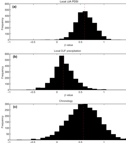
and pluvials even in the presence of a seasonality in rain-fall sensitivity or mixed climate response (Cook et al., 1999). Franke et al. (2013) and Bunde et al. (2013) raised concerns about the spectral fidelity of tree-ring proxies, observing that the slope of their frequency continuum resembled neither that of temperature nor precipitation; however, a reexamina-tion of the coeval spectra of a global network of tree-ring chronologies presented here in Fig. 2 suggests that this ap-parent discrepancy is because hydroclimate tree-ring proxies reflect soil moisture, which displays greater power at decadal to centennial frequencies. In a related example, Wahl et al. (2017) developed spatially explicit annual precipitation re-constructions for the western United States, which exhibit the same spectral characteristics as the corresponding instru-mental data. The approach used existing river flow recon-structions as the predictor data to explicitly take advantage of the integrated moisture balance signal reflected in river flow.
−10 −0.5 0 0.5 1 1.5 100
200 300 400 500 600
β value
Freq
uency
−10 −0.5 0 0.5 1 1.5
100 200 300 400 500 600
β value
Local DJF precipitation
−10 −0.5 0 0.5 1 1.5
50 100 150 200 250 300
β value
Chronology
(a)
(b)
(c)
Freq
uency
Freq
uency
[image:7.612.85.513.69.555.2]Local JJA PDSI
Figure 2. The slope of the multitaper spectrum expressed asβvalue (Huybers and Curry, 2006) for climate and tree-ring variables at locations with tree-ring chronologies from the North American Drought Atlas (Cook et al., 1999, 2010b), the Monsoon Asia Drought Atlas (Cook et al., 2010a), the Old World Drought Atlas (Cook et al., 2015b), and the Mediterranean and North Africa (Touchan et al., 2011, 2014).(a)β-value frequency distribution for summer (JJA) PDSI from van der Schrier et al. (2011) at tree-ring chronology locations,(b) β-value frequency distribution for winter (DJF) GPCC precipitation (Schneider et al., 2014) at tree-ring chronology locations, and(c)for the tree-ring chronologies themselves. All data were normalized [0,1] over their common interval and theirβvalues were calculated using the multitaper method (Thomson, 1982).
2.3 Speleothems
Speleothems (e.g., stalagmites, stalactites) are cave deposits that form when calcium carbonate precipitates from de-gassing solutions as they seep into limestone caves, leaving
and 234U, to provide absolute chronologies for stalagmite-based paleoclimate records (Edwards et al., 1987; Cheng et al., 2000) with precisions of<1 % (2 sigma; Shen et al., 2012) over the last∼650 thousand years (e.g., Cheng et al., 2016b). Stalagmite-based paleoclimate records typically re-solve millennial- to orbital-scale variations in climate at a given site, owing to their slow and often steady growth averaging 2–20 µm yr−1 over many tens of millennia. Cur-rently, numerous absolutely dated, well-replicated stalagmite
δ18O records with decadal to centennial resolution exist from South America (Cruz et al., 2005; Wang et al., 2007), the western Pacific (Partin et al., 2007; Griffiths et al., 2009, 2010; Meckler et al., 2012; Carolin et al., 2013; Griffiths et al., 2016), China (Wang et al., 2001; Zhang et al., 2008; Cheng et al., 2016a), and the Eastern Mediterranean and Middle East (Bar-Matthews et al., 1997; Bar-Matthews et al., 1999; Fleitmann et al., 2007, 2009; Cheng et al., 2015; Flohr et al., 2017).
The generation of sub-annual to annually resolved stalag-mite records holds immense potential to reconstruct hydro-climate conditions in many regions through the CE. In most cases, such high-resolution records rely on 10–500 µm sam-pling of unusually fast-growing stalagmites that form on the order of 100–2000 µm yr−1(Treble et al., 2003; Partin et al., 2013; Chen et al., 2016). Even for these fast-growing records, however, the period of the CE may only span several cen-timeters to, in exceptional cases, many tens of cencen-timeters, ultimately limiting the number of 1–2 mm scale samples that can be drilled for conventional, high-precision U/Th dating. In many cases, stalagmite growth rates also vary significantly over the CE, and/or growth can slow to near-zero values, causing a hiatus that can be poorly resolved by the rela-tively small number of available U/Th dates. These circum-stances represent a significant challenge to the generation of age models for stalagmites spanning the CE based on radio-metric dates. Two programs – BChron (Haslett and Parnell, 2008) and StalAge (Scholz and Hoffmann, 2011) – allow researchers to calculate age models and their uncertainties for stalagmite records given a set of radiometric dating con-straints, including the identification of potential hiatuses (see Scholz et al. (2012) for a review of age modeling approaches to speleothem records). In rare cases, annually banded sta-lagmites afford the generation of layer-counted chronologies that can be tested against radiometric ages (Polyak et al., 2001), although recent work has demonstrated that apparent annual banding in stalagmites may not always be strictly an-nual (Shen et al., 2013).
The most widely used and best-understood measurement for speleothem-based climate reconstructions is the oxygen isotopic composition, or δ18O, of calcite (e.g., Fleitmann et al., 2004), which under constant precipitation conditions reflects changes in cave temperature and changes in theδ18O of the cave dripwater feeding the stalagmite. Over the CE, air temperature in a given cave likely changed very little (<1◦C or∼0.2 ‰ in stalagmiteδ18O units) such that the observed
speleothemδ18O variations of up to 1 ‰ are governed pri-marily by groundwaterδ18O variability. In most scenarios, groundwaterδ18O composition reflects a weighted mean of rainfall δ18O averaged over the preceding months in wet environments (Moerman et al., 2014), while it may reflect years in semiarid and arid environments (Ayalon et al., 1998). Some studies also show that recharge of the aquifer occurs only during months when rainfall passes a given threshold, typically during the wet season in the tropics (e.g., Jones and Banner, 2003; Partin et al., 2012), but possibly associ-ated with the winter storm season in the extratropics. While other indicators, such as band thickness (e.g., Rasbury and Aharon, 2006; Asmerom et al., 2007), trace metal ratios (see Fairchild and Treble, 2009 and references therein), and car-bon isotopes (Fairchild et al., 2000; Frappier et al., 2002; Os-ter et al., 2015) reflect hydroclimate variability at certain sites and continue to be developed, speleothemδ18O remains the primary hydroclimate proxy.
Modern studies of rainfall δ18O, cave dripwater δ18O, rainfall amount, and speleothem δ18O show that, depend-ing on the location, speleothemδ18O may be a record of lo-cal rainfall amount, regional hydroclimate variability, and/or changes in the source of the moisture that is linked to re-gional hydroclimate variability (e.g., Flohr et al., 2017 and references therein). In the past, the so-called “amount effect” was invoked to interpret a speleothemδ18O record (Dans-gaard, 1964), which assumed an inverse, empirical relation-ship between rainfall amount and rainfall δ18O (Rozanski et al., 1993; Gat, 1996). Over the tropical ocean or over small tropical islands, the amount effect dominates the rela-tionship on monthly to interannual timescales (Kurita, 2013), whereby local rainfallδ18O reflects the cumulative fraction-ation of water isotopes over the transit of the vapor par-cel through space and time. As such, many calibration ef-forts demonstrate that speleothem δ18O is inversely corre-lated with the instrumental rainfall at the site on annual to decadal timescales (e.g., Partin et al., 2013). In other loca-tions, rainfallδ18O and cave dripwaterδ18O correlate better with indices of large-scale circulation patterns (e.g., ENSO indices) than with local rainfall amount (Moerman et al., 2013, 2014). Lastly, some studies show that speleothemδ18O can reflect changes in the source of precipitation, which al-ters theδ18O of rainfall (Aggarwal et al., 2004; Breitenbach et al., 2010). Unified frameworks and theories are now being tested to determine the underlying mechanisms controlling rainfallδ18O in order to more directly compare rainfall out-put from climate models with speleothemδ18O records (e.g., Lewis et al., 2010; Aggarwal et al., 2012; Jones et al., 2016; Tharammal et al., 2017). These efforts are also relevant for other proxy records of precipitationδ18O andδD, for exam-ple sediments (Sect. 2.4) and coral records that are sensitive to the isotopic composition of rainfall (Sect. 2.1).
Cheng et al., 2012; Denniston et al., 2015; Cai et al., 2017). A recent paper by Hu et al. (2017) pointed out several chal-lenges that especially apply over the CE, including serial autocorrelation, the test multiplicity problem in connection with a climate field, and the presence of age uncertainties. Hu et al. (2017) include information and code on how to address these issues when interpreting a record. Additionally, PSMs (see Sect. 4 for more discussion) are used to simulate deposi-tional processes, which can incorporate karst processes that may redden the karst signal (Dee et al., 2015). Such stud-ies indicate that even in the simplest of karst models, signal reddening and the impacts of high- to low-frequency signal enhancement can be captured and explained (Partin et al., 2013).
Finally, an expanding network of speleothem records is being compiled and characterized by the PAGES2k Trans-Regional Project, Iso2k (Partin et al., 2015). This effort has identified over 65 published records of speleothem-based hy-droclimate estimates over the CE. These records span ev-ery major continent outside of Antarctica. Continuing co-ordinated efforts to generate well-replicated, high-resolution records of speleothemδ18O that span all or part of the CE will yield robust reconstructions of hydroclimate that can be directly compared to the expanding number of simulations spanning the CE, some of which are isotope equipped (and more are expected as part of the CMIP6 archive).
2.4 Sediments
Marine and lacustrine sediment cores play an important role in the reconstruction of past hydroclimate variability over the CE, as they often extend further back in time than corals and tree rings. There are typically multiple hydroclimate proxies that can be measured in any given sediment core, theoreti-cally allowing for better isolation of the climatic signal from noise. Such proxies include the following:
Lake level indicators: Inference of past lake levels, particu-larly from closed-basin lakes, serves as a sensitive indictor of P–E and therefore regional moisture balance (cf. Verschuren et al., 2000; Shuman et al., 2009; Xu et al., 2016; Goldsmith et al., 2017).
Pollen and other microfossil transfer functions: Micro-fossil assemblages such as pollen and diatoms can be di-rectly regressed against modern climatic variables such as P–E or mean annual precipitation. A number of statistical approaches may be employed, such as the modern analog technique (e.g., Overpeck et al., 1985), artificial neural net-works (e.g., Peyron et al., 1998), variation partitioning and redundancy analysis (e.g., Li et al., 2017), and hierarchical Bayesian models (Haslett et al., 2006).
Runoff indicators: Physical and chemical characteristics of lake and marine sediments, such as the concentration of ma-jor elements (Ti, Fe, Ca) or grain size, can be used to in-fer runoff intensity, which is in turn related to the intensity, frequency, or amount of rainfall. Scanning XRF techniques
make it possible to analyze such characteristics at very high temporal resolution (e.g., Haug et al., 2001, 2003; Moreno et al., 2008).
Proxies for water isotopes: In marine cores, measurement of theδ18O of surface-dwelling foraminifera provides insight into hydroclimatic change over the ocean, just asδ18O does in corals (see Sect. 2.1). Simultaneous measurement of the Mg/Ca ratio in foraminifera gives an independent constraint on temperature, allowing for the isolation of the signal asso-ciated with the δ18O of seawater (Elderfield and Ganssen, 2000). In both marine and lacustrine sediments, measure-ments of the hydrogen isotopic composition of lipids from aquatic algae and terrestrial higher plants can be used to re-construct sea- or lake-waterδD and precipitationδD, respec-tively (e.g., Sachs et al., 2009; Tierney et al., 2010; Richey and Sachs, 2016). Such proxies provide important constraints on processes that influence isotopes of precipitation, such as rainfall amount, source, and seasonality.
The diverse and independent proxy systems available are a clear strength of sedimentary archives. Nevertheless, work-ing with sediment records on recent timescales presents a number of challenges that must be considered when inter-preting data and incorporating them into a multi-proxy recon-struction framework. An obstacle inherent to working with sediments is the uncertainty related to chronology – that is, the assignment of depth horizons to points in time. Varved sediments (sediments in which distinct layers are deposited on a demonstrably annual basis) have relatively tightly con-strained chronologies, although counting errors will prop-agate downcore, as is the case with any annually layered archive that is not cross-dated (Comboul et al., 2014). Varves are nevertheless rare in marine environments and in the ter-restrial tropics, and in their absence chronological assign-ment depends on radiometric methods. The two most com-mon systems used in dating recent marine sediments are 210Pb and14C. With a half-life of 22.2 years,210Pb is ideal
for dating sediments spanning the last 100–150 years and can provide an accuracy ranging from 1–20 years. Older sediments are dated primarily with14C, which has a half-life of 5730 years. In lakes,14C may be measured on ter-restrial macrofossils or bulk organic carbon, although the latter can be affected by the presence of old carbon (com-ing from, for example, an isolated hypolimnion or terrestrial CaCO3 input). In marine sediments, 14C is typically mea-sured on species of planktonic foraminifera. In this case, one must account for the14C age of the ocean water (ca. 200– 1500 years) or the marine “reservoir effect”. Globally, the average 14C age of ocean water is 400 years (Stuiver and Braziunas, 1993). Local deviations from this age are com-monly expressed as1R, the values of which are determined by measuring the14C age of contemporary known-age, pre-nuclear marine specimens such as bivalves and corals.
Figure 3.Examples of the effect of age model uncertainty and spectral reddening on paleoclimate signatures in sedimentary archives.(a)Age model uncertainty associated with the Lake Naivasha (East Africa) lake level record (Verschuren et al., 2000) spanning the last millennium. Data on the published age model are plotted in black. Blue regions represent the 1σ and 2σ uncertainty bounds for the dating of the data, applying a Monte Carlo method for iterating age model uncertainty (Anchukaitis and Tierney, 2013). Red triangles denote the locations of chronological constraints (dates). Note that the timing of lake overflow during the Little Ice Age may have occurred anytime between 1600 and 1800 CE. Figure after Tierney et al. (2013).(b)Comparison of historical monthly precipitation (from the Global Historical Climatology Network; Peterson and Vose, 1997) and lake level data (from Stager et al., 2007) for Lake Victoria, East Africa. Both the precipitation and the lake level data are from Jinja, Uganda. Note the step-change response of lake level to an extreme rainfall event in 1961. Inset shows a comparison of the power spectra; note the loss of high-frequency and increase in low-frequency power in the lake level data compared to precipitation.
the 14C calibration curve (placement on a radiocarbon pro-duction “plateau” will increase error), and uncertainties in reservoir corrections (see example in Fig. 3a). Thus, over the timeframe of the CE, chronological uncertainties can be formidable. Increased density of dating and independent con-straints on sedimentation rates can improve the precision of the chronology, but multiple age–depth models are always possible. This uncertainty is best dealt with through an en-semble approach, i.e., the use of a Monte Carlo or Bayesian age modeling method to produce a posterior ensemble of age–depth models that can then be used iteratively in a recon-struction framework (Ramsey, 2008; Blaauw and Christen, 2011; Anchukaitis and Tierney, 2013; Tierney et al., 2013; Werner and Tingley, 2015).
Another special consideration for sedimentary archives is the role of bioturbation. In low-oxygen environments, sedi-ments may be deposited essentially “undisturbed” and will appear laminated. In most locations, however, bottom water oxygen is present and the benthos (organisms living on and in the seafloor) will mix the upper layers of the sediment. In the ocean, bioturbation depths average 8 cm globally but vary from 0–20 cm depending on productivity, bottom water oxy-gen, and sedimentation rate (Teal et al., 2008). Bioturbation
thus acts as a low-pass filter on sedimentary proxy signatures and will redden the spectra of proxy time series. Diffusion-based forward models for bioturbation exist and can be incor-porated into reconstruction frameworks (e.g., Trauth, 2013). The proxy systems in sediment archives also have the ca-pability to redden the spectra of paleoclimate signatures, and this must be considered both for inter-archive and proxy– model data comparisons. Lake level records, for example, are typically low-pass-filtered representations of regional hydro-climate. Lake water residence time and hydraulic considera-tions buffer variability in P–E such that lake levels will have more power at low frequencies and less at high frequencies than the local climate variable (see example in Fig. 3b). The amount of reddening depends on individual lake systems and can be forward modeled if lake geometry, inputs, and outputs are known (e.g., Hurst, 1951; Hostetler and Benson, 1994).
or pluvials and complement higher-resolution perspectives from other hydroclimatic proxies.
2.5 Documentary evidence
Documentary evidence includes noninstrumental informa-tion on past climate and weather condiinforma-tions before the ad-vent of continuous meteorological measurements, the prin-cipal sources of which are descriptive documentary data (i.e., descriptive observations of weather, reports from chron-icles, ship logbooks, travel diaries, etc.) and documentary proxy data. This latter source of information refers to indi-rect records of events or practices tied to specific weather events or climatic conditions; examples include the begin-ning of agricultural activities, the freeze and thaw dates of waterways, records of floods, and reports of religious cere-monies in response to impactful meteorological conditions (see Brazdil et al., 2005, for a review).
Descriptive evidence generally has good dating control and high temporal resolution (for specific periods and re-gions, even daily resolution is possible), but this evidence is also typically discontinuous. Documentary sources also tend to emphasize extreme events because the consequences of their socioeconomic impacts render them more likely to have been recorded (Brazdil et al., 2005). Typical exam-ples include hydrometeorological extremes (flooding, hail, torrential rains) and other natural hazards that impacted the success of harvests or placed livestock in jeopardy (Pfister et al., 1999; Camenisch et al., 2016). China, Japan, and Eu-rope comprise the three main geographic regions where an abundance of historical climatological sources exist. More recently, assessments have been initiated for records from South America that date back to the beginning of Spanish colonization (Neukom et al., 2010). Data from Africa, North America, and Australia are available for much shorter pe-riods into the past in comparison with other regions where more abundant documentary data exist (e.g., Grab and Nash, 2010; Nash and Grab, 2010; Fenby and Gergis, 2013; Gergis and Ashcroft, 2013; Neukom et al., 2014; Nash et al., 2016).
2.5.1 Europe
Research on documentary-based past hydroclimate in Eu-rope is temporally and geographically heterogeneous (e.g., Brazdil et al., 2005; Pauling et al., 2006). Potentially useful documentary evidence is available in most of Europe and the Mediterranean regions, although only a few regions include hydroclimatic studies (including droughts, floods, and other extremes), these being in the Czech Republic, Germany, the eastern Mediterranean, Byzantium, Hungary, Italy, Portugal, Spain, Switzerland, and the UK (Brazdil et al., 2005, 2010, 2012, 2013, 2016; Luterbacher et al., 2006; Wetter et al., 2011, 2014; Dobrovolny et al., 2015; Mozny et al., 2016; Xoplaki et al., 2016; Domínguez-Castro et al., 2008, 2014; Barriendos et al., 2003, 2014; Todd et al., 2013; Benito et
al., 2015; Himmelsbach et al., 2015). New and promising data from other regions do exist, but they have not yet been fully explored. Some records prior to 1000 CE (e.g., Xoplaki et al., 2016 and references therein) are available during the Byzantine Empire (including the Balkans) and the Carolin-gian Empire. Subsequent to 1000 CE, specific periods can be characterized (Brazdil et al., 2005; Pfister et al., 2008) that include a progression from individual reports of significant socioeconomic anomalies and disasters (weather induced, floods, droughts) from 1000–1200 CE to almost full descrip-tions for monthly weather (including some daily weather and extremes) from 1500–1800 CE. From around 1650 through 1860 CE, early instrumental measurements made by individ-uals and organized by scientific and economic societies be-come available. These earlier efforts are followed by short-lived international instrumental networks (up to the end of the 18th century) and initiatives within 19th century emerg-ing nation states.
Despite the relative abundance of information in Eu-rope, our understanding of hydroclimate variability (includ-ing short-duration and extensive drought and flood periods) is still limited because only a small number of well-dated documentary proxy records with high temporal resolution are available and because they are unevenly distributed over the continent (e.g., Brazdil et al., 2005). Some synthesis efforts have nevertheless been pursued. Pauling et al. (2006) and Carro-Calvo et al. (2013) combined early instrumental series, documentary proxy time series, and natural proxies to recon-struct seasonal precipitation fields for European and Mediter-ranean land areas covering the past half millennium. A sim-ilar reconstruction was provided by Casty et al. (2007), who used only documentary and natural proxies tied to precipi-tation, which allows for comparison to independently recon-structed temperature and pressure fields. Collectively, identi-fying and characterizing historical extreme events that have severely stressed human or natural systems (e.g., the onset, duration, frequency, and intensity of droughts and floods) is a critical endeavor, and our capacity for studying these events is possible through the continued development and interpre-tation of documentary records in Europe.
2.5.2 Asia
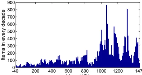
re-Figure 4.The amount of climatic information extracted from Chi-nese classical documents (a reproduction of Fig. 7 in Ge et al., 2008b).
constructions. Qualitative reconstructions are generated by counting the number of dry and wet events, which occasion-ally consider the timing, scale, and severity of these events based on written descriptions in a wide range of historical papers (Gong and Hameed, 1991; Ge et al., 2016). Numerous reconstructions in this class have been published, for instance D–W series for 120 subregions across China from 1470– 2000 CE (CMA, 1981; Zhang et al., 2003), a regional D–W dataset from 960–1992 CE (Zhang et al., 1997), a 1000-year D–W dataset for the Guanzhong Plain (Hao et al., 2017), the history of moisture conditions for the last 2000 years (Gong and Hameed, 1991), D–W series for 63 sites since 137 BCE (Zhang, 1996), and a relatively new D–W dataset for the pe-riod 501–2000 CE that has been subsequently extended to cover the last 2000 years (Zheng et al., 2006, 2014). The characteristics of droughts and floods based on these records have been extensively studied, such as the frequency, sever-ity, spatial patterns, and decadal to centennial variability of hydroclimate, as well as the relationship between D–W in-dices and temperature (e.g., Wang and Zhao, 1979; Zhang and Crowley, 1989; Yan et al., 1992; Qian et al., 2003; Shen et al., 2009; PAGES 2k Consortium, 2013).
For quantitative reconstructions, around 300 years of an-nual and/or seasonal precipitation time series are available in northern China and the mid-lower Yangtze River valley (Zhang and Liu, 2002; Zhang et al., 2005; Zheng et al., 2005) using accurate weather and climate descriptions from “Qing Yu Lu” (clear and rain records), “Yu Xue Fen Cun” (rainfall infiltration and snowfall depth, Ge et al., 2005), and others. Qualitative precipitation reconstructions have been used to study meiyu (plum rain) activity (Zhang and Wang, 1991; Ge et al., 2008a; Ding et al., 2014a), an exceptional flood-ing event in 1755 CE (Zhang et al., 2013), and East Asian summer monsoon variations at multidecadal and centennial scales (Hao et al., 2015). Because quantitative precipitation reconstructions over China are relatively short and spatially limited, researchers have tried to provide quantitative pre-cipitation information by combining D–W indices and other
high-resolution proxies. For example, by incorporating D–W indices and tree-ring proxies, Yi et al. (2012) reconstructed annual summer precipitation in north-central China back to 1470 CE, and Feng et al. (2013) generated a gridded recon-struction of warm season precipitation over Asia spanning the last 500 years. Some of these Chinese efforts are comple-mented by efforts in Japan – many documents dating from the Edo era (1603–1868 CE) contain records of daily weather conditions. The majority of the known daily weather records have been digitized and added to the Historical Weather Database of Japan (Mikami, 1988, 2008). Other long doc-umentary records come from phenological information from Kyoto (Aono and Kazui, 2008) and from direct human ob-servations of freezing dates for Lake Suwa, Japan (Sharma et al., 2016, and references therein).
3 Coupled model simulations of the Common Era
In concert with hydroclimate proxy development over the last several decades, efforts to model the CE have also pro-gressed considerably. In the last decade, two complementary approaches have enhanced the relevance of paleoclimate sim-ulations for our understanding of past climate evolution. The first is the use of single-model ensembles (Jungclaus et al., 2010; Hofer et al., 2011; Otto-Bliesner et al., 2016) com-prising multiple simulations with the same model configura-tion and experimental design (i.e., Schmidt et al., 2011; Otto-Bliesner et al., 2016). These ensemble frameworks allow for the systematic characterization of simulated internal climate variability and forced responses, as well as an assessment of uncertainties in boundary forcing estimates. Single-model ensembles are nevertheless subject to the peculiarities and deficiencies of the individual model used.
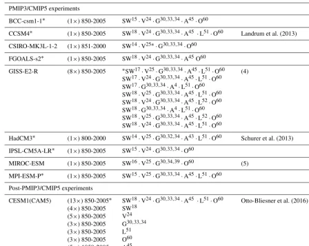
[image:12.612.49.284.72.197.2]Table 1.PMIP3/CMIP5 and post-PMIP3/CMIP5 simulations of the CE and their associated forcings.
PMIP3/CMIP5 experiments
BCC-csm1-1∗ (1×) 850-2005 SW15·V24·G30,33,34·A45·O60
CCSM4∗ (1×) 850-2005 SW18·V24·G30,33,34·A45 ·L51·O60 Landrum et al. (2013)
CSIRO-MK3L-1-2 (1×) 851-2000 SW14·V25∗·G30,33,34·O60
FGOALS-s2∗ (1×) 850-2005 SW18·V24·G30,33,34·A45O60
GISS-E2-R (8×) 850-2005 ∗SW17·V25·G30,33,34·A45·L51·O60 SW17·V24·G30,33,34·A45·L51·O60 SW17·G30,33,34·A4·L51·O60 SW18·V25·G30,33,34·A45·L51·O60 SW18·V24·G30,33,34·A45·L52·O60 SW18·G30,33,34·A4·L51·O60 SW18·V25·G30,33,34·A45·L52·O60 SW18·V24·G30,33,34·A45·L51·O60
(4)
HadCM3∗ (1×) 800-2000 SW14·V25·G30,32,34·A43·L51·O60 Schurer et al. (2013)
IPSL-CM5A-LR∗ (1×) 850-2005 SW15·V24·G30,33,34·O60
MIROC-ESM (1×) 850-2005 SW16·V25·G30,34,39·O60 (5)
MPI-ESM-P∗ (1×) 850-2005 SW15·V25·G30,33,34·A45·L51·O60
Post-PMIP3/CMIP5 experiments
CESM1(CAM5) (13×) 850-2005∗ (4×) 850-2005 (5×) 850-2005 (3×) 850-2005 (3×) 850-2005 (3×) 850-2005 (5×) 1850-2005
SW18·V24·G30,33,34·A45 ·L51·O60 SW18
V24 G30,33,34 L51 O60 A45
Otto-Bliesner et al. (2016)
(1) Key for superscript indices in forcing acronyms:
[1]Solar:
[14]Steinhilber et al. (2009) spliced to Wang et al. (2005).
[15]Vieira and Solanki (2010) spliced to Wang et al. (2005).
[16]Delaygue and Bard (2011) spliced to (Wang et al., 2005).
[17]Steinhilber et al. (2009) spliced to Lean et al. (2005).
[18]Vieira et al. (2011) spliced to Lean et al. (2005).
[2]Volcanic:
[24]Gao et al. (2008). In the GISS-E2-R simulations this forcing was implemented twice as large as in Gao et al. (2008).
[25]Crowley and Unterman (2013). In the CSIRO simulation this forcing was implemented as a global mean reduction in total solar irradiance.
[3]GHGs:
[30]Fluckiger et al. (1999); Fluckiger et al. (2002); Machida et al. (1995).
[32]Johns et al. (2003).
[33]Hansen and Sato (2004).
[34]MacFarling Meure et al. (2006).
[39]CO2diagnosed by the model. [4]Aerosols:
[43]Johns et al. (2003).
[45]Lamarque et al. (2010).
[5]Land use, land cover:
[51]Pongratz et al. (2009) spliced to Hurtt et al. (2006).
[52]Kaplan (2011).
[6]Orbital:
[60]Berger (1978).
3.1 Simulating hydroclimate over the Common Era
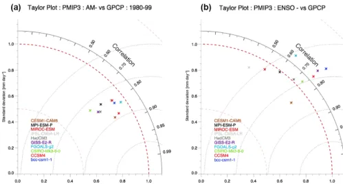
In general, climate models do not simulate hydroclimatic variables, such as precipitation, as realistically as surface temperatures (Flato et al., 2013; e.g., Fig. 5a). This is due
represen-Figure 5.Taylor diagrams of global precipitation over land(a)and ENSO (as defined by the Nino3.4 index) correlations to precipitation over land(b). Each panel shows models that completed PMIP3 simulations of the last millennium compared to precipitation observations from GPCP for the overlapping periods of 1980–1999(a)1980–2014 for(b)(not all models simulated the full period, but all are at least 1980–2004).
tation of hydroclimatic impacts associated with modes of variability (Davini and Cagnazzo, 2014; see Fig. 5b). Nev-ertheless, models are generally successful at simulating the large-scale atmospheric circulations that drive areas of subsi-dence and uplift, and thus generally represent the zonal mean hydroclimate well, particularly in the multi-model ensemble mean (Flato et al., 2013). This is less true of regional hy-droclimate dynamics, as many models struggle to reproduce the full characteristics of observed phenomena such as the global monsoon systems (e.g., Geil et al., 2013; Langford et al., 2014, for the North American monsoon; Sperber et al., 2013, for the Asian monsoon), some midlatitude storm tracks and the frequency of associated cyclonic systems (e.g., in the western and northern Atlantic; Colle et al., 2013; Dunn-Sigouin and Son, 2013; Sheffield et al., 2013; Zappa et al., 2013), and atmospheric blocking (Masato et al., 2013). A full consideration of hydroclimate also includes the representa-tion of land surface processes. While hydrology, vegetarepresenta-tion, and soil moisture modeling has become increasingly com-plex, these components of models have not been as widely validated, and paleoclimate simulations often do not include important processes such as dynamic vegetation (Braconnot et al., 2007, 2012). To overcome some of these challenges, regional climate model simulations are used where processes important for simulating hydroclimate are better resolved. Due to the high computational demand, however, few
re-gional modeling studies have been applied in the context of proxy–model comparisons over the CE. Gómez-Navarro et al. (2015) is one of the few examples of a regional simu-lation study for Europe that has been used to assess drought indices (Raible et al., 2017), covariability of seasonal tem-perature and precipitation (Fernandez-Montes et al., 2017), and the interpretation of lake sediments (Hernandez-Almeida et al., 2017).
[image:14.612.47.546.63.331.2]At the continental scale, Ljungqvist et al. (2016) presented a spatial reconstruction of NH hydroclimate variability for the last 1200 years and compared the data with PMIP3 last-millennium simulations. They discussed the relationship be-tween long-term temperature evolution and hydroclimate and diagnosed a statistically significant covariability for partic-ular regions, but also widespread deviations from this rela-tionship. In particular, the authors found that reconstructions and simulations agree reasonably well over the preindustrial interval and indicate that the 13th century had the most ex-tensive dry conditions. Attribution to external forcing could, however, not be obtained from the assessment.
Models are also capable of reproducing multidecadal drought periods in some arid regions, a prominent and socioeconomically relevant feature of past hydroclimate variations. For instance, Coats et al. (2015b) analyzed megadroughts in the American Southwest in proxy recon-structions and in PMIP3 simulations, finding that models can reproduce events that are similar in extent and severity to tree-ring-derived reconstructions. The authors neverthe-less also described pronounced differences between paleo-climatic reconstructions and models. For example, not all of the PMIP3 models associate megadroughts with teleconnec-tions originating in the tropical Pacific Ocean, which is the assumed origin in the real climate system, and therefore may not accurately represent the dynamics underlying real-world megadroughts (Coats et al., 2016a, b). Conversely, internal atmospheric variability and land surface coupling may have instead been the dominant mechanism behind the occurrence of many megadroughts (Stevenson et al., 2015b). Whereas Coats et al. (2015b) diagnosed the general ability of climate models to reproduce low-frequency hydroclimate variability from a dynamical perspective, other studies based on statis-tical rescaling (Ault et al., 2012) find that model simulations underestimate low-frequency (in the 50 to 200 year range) precipitation variability. Spectra of reconstructed hydrocli-matic variables from western North America show a consid-erably “redder” characteristic than those from models (Ault et al., 2013a). These findings are also tied to interpretations of proxy spectral fidelity, as discussed in Sect. 2.
3.2 Natural forcing of hydroclimate
Natural exogenous forcing factors have led to hydroclimate variability during the CE; the strongest influences are vol-canic eruptions and changes in solar activity. The former, namely stratospheric aerosols from strong volcanic erup-tions, is the most important of these two forcings at the global scale during the preindustrial interval of the CE. Although the impacts persist for only a few years, volcanic forcing from multiple events constitutes the most important contrib-utor to the global centennial-scale cooling observed from 850–1800 CE based on comparisons of single-forcing ex-periments (Otto-Bliesner et al., 2016) or through the use of all-forcing simulations in which the contributions from
in-dividual forcings are isolated offline (Atwood et al., 2016). For this reason, volcanic eruptions are particularly impor-tant for gauging the forced hydroclimatic response in last-millennium simulations.
Both observational and modeling studies consistently find a decrease in global precipitation following large explosive eruptions; the main regions experiencing decreased precipi-tation tend to be the tropics (Robock and Liu, 1994; Yoshi-mori et al., 2005; Trenberth and Dai, 2007; Schneider et al., 2009) and monsoon regions (Schneider et al., 2009; Joseph and Zeng, 2011; Wegmann et al., 2014; Stevenson et al., 2016). Iles and Hegerl (2014) further examined the precip-itation response to volcanic eruptions in the CMIP5 histor-ical simulations compared to three observational datasets. Global precipitation significantly decreases following erup-tions in CMIP5 models, with the largest decrease in wet trop-ical regions. Iles et al. (2013) examined the global precipita-tion response to large low-latitude volcanic erupprecipita-tions using an ensemble of last-millennium simulations from HadCM3 that indicated a significant reduction in global mean pre-cipitation following these events. In the tropics, areas ex-periencing post-eruption drying coincide with climatologi-cally wet regions, while dry regions get wetter on average, but the changes are spatially heterogeneous; a similar pat-tern has also been noted over Europe (Rao et al., 2017). These responses are physically consistent with future global warming projections, but of opposite sign because volcanoes and greenhouse gases have contrasting influences on radia-tive forcing. It must also be noted that the general pattern of wet regions getting wetter and dry regions getting drier in re-sponse to warming forced by increasing greenhouse gases is not universally applicable and can break down, particularly over land and in the tropics (Chou et al., 2009; Scheff and Frierson, 2012; Chadwick et al., 2013; Huang et al., 2013; Byrne and O’Gorman, 2015).
Despite earlier studies, substantial uncertainties still af-fect our understanding of hydroclimate responses to vol-canic forcing in certain tropical regions. For instance, the CMIP5/PMIP3 last-millennium ensemble does not robustly feature the persistent drying over Mesoamerica that was de-tected in a recent speleothem record and ascribed to volcani-cally induced changes in dominant modes of variability in the tropical Pacific and Atlantic, including ENSO (Winter et al., 2015). There are still apparent discrepancies in proxy-derived hydroclimate responses to volcanic eruptions in Asia and those simulated by several models (e.g., Anchukaitis et al., 2010) although it is not clear whether this is due to poorly simulated dynamics (and, if so, what dynamics are not adequately treated), uncertainties in forcing estimates, large contributions from internal variability, or deficiencies in the interpretation of the proxy network (Stevenson et al., 2016, 2017).
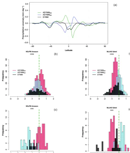
demonstrated that the response of the Intertropical Conver-gence Zone (ITCZ) differs dramatically for aerosol loading centered in the Northern vs. the Southern Hemisphere in the Community Earth System Model (CESM) Last Millennium Ensemble (LME) and NASA ModelE2-R last-millennium simulations (Table 1), with the ITCZ shifting away from the hemisphere with the greater concentration of aerosols (Hay-wood et al., 2013). Liu et al. (2016) also classified volcanic eruptions based on their meridional aerosol distributions and noted that NH volcanic eruptions are more efficient in re-ducing NH monsoon precipitation than SH eruptions. Fig-ure 6a characterizes precipitation anomalies after volcanic eruptions, while Fig. 6b and d separate the precipitation re-sponse to the volcanic forcing of differing meridional struc-tures in CESM LME (18 ensemble members; see Colose et al. (2016a) for details on eruption classifications) during boreal winter in the Amazon and boreal summer in the Sahel, respectively. Although there is considerable spread within a given classification related to different eruption magnitudes and internal variability, there is a strong tendency for an in-crease in local precipitation if the aerosol loading is pref-erentially located in the opposite hemisphere. Unique local responses to different volcanic eruptions, even for a partic-ular configuration of the atmospheric state, should therefore not be expected. Figure 6c and e show the same result us-ing all eruptions within three ensemble members in NASA GISS ModelE2-R. Volcanic eruptions were incorrectly im-plemented in these three simulations (those using Gao et al., 2008) such that the aerosol optical depth for all events is approximately 2 times too large (Masson-Delmotte et al., 2013), but the implementation fortuitously allowed for an analysis of events with a very large signal.
In addition to the spatial distribution of volcanic aerosols, descriptions of volcanic aerosol cloud properties are also critical for simulations of the hydroclimate response to past eruptions. Substantial differences exist between reference volcanic forcing datasets in terms of overall aerosol load-ing and their latitudinal structure (Gao et al., 2008; Crow-ley and Unterman, 2013; Sigl et al., 2015). The differ-ences include the timing, magnitude, and spatial structure of the forcing, as well as the reported variable (e.g., AOD or aerosol mass). Furthermore, implementation of a given forcing dataset may differ among modeling groups, for in-stance by varying the aerosol effective radius (Crowley and Unterman, 2013; Zanchettin et al., 2016). Other understud-ied aspects of uncertainties in eruption characteristics may also play a substantial role in hydroclimate impacts, such as plume composition, vertical profiles (LeGrande et al., 2016), and the initial month of eruptions; the latter is often assumed constant, but variability in the timing of eruptions has a sig-nificant controlling influence on the structure of forced hy-droclimate anomalies (Stevenson et al., 2017). A consider-ation of the forcing implementconsider-ation is therefore critical for meaningful proxy–model comparisons and adds a dimension
of uncertainty that is independent of model skill or the cli-matic interpretation of the proxies of interest.
The robustness of the ENSO response following volcanic eruptions has been a longstanding subject of inquiry and rep-resents another important dynamic response that needs to be better understood in the context of hydroclimatic responses to volcanic events. Many studies have yielded equivocal re-sults, with some arguing that eruptions bias the tropical hy-droclimate state toward El Niño conditions (e.g., Mann et al., 2005; Emile-Geay et al., 2008; Li et al., 2013; Wahl et al., 2014; Maher et al., 2015) or toward La Niña conditions (D’Arrigo et al., 2008, 2009; McGregor and Timmermann, 2011; Zanchettin et al., 2012); others argue that there is no evidence of an ENSO response to volcanic forcing (Robock and Mao, 1995; Self et al., 1997; Ding et al., 2014b; Tierney et al., 2015a). More recently, Pausata et al. (2016) have ar-gued that eruptions with preferential aerosol loading in the NH will generate El Niño conditions by virtue of a south-ward ITCZ shift, which slackens the trade winds over the Pacific Ocean. The tendency for NH eruptions to favor initi-ation of El Niño was also found by Stevenson et al. (2016) in the CESM LME; in contrast, eruptions with stronger aerosol loading in the SH tend to suppress El Niño conditions during the following winter. Predybaylo et al. (2017) investigated the ENSO response to a Pinatubo-sized eruption using the GFDL–CM2.1 coupled climate model under different initial ENSO conditions and eruption seasons and identified a sta-tistically significant El Niño response in the year after erup-tion for all initial ENSO condierup-tions except La Niña. Steven-son et al. (2016) also used the CESM LME to investigate the separate influences of volcanic eruptions and ENSO on hy-droclimate variability. Hyhy-droclimate anomalies in monsoon Asia and the Western United States resemble the El Niño teleconnection pattern following volcanic forcing that is ei-ther symmetric about the Equator or preferentially located in the NH. El Niño events following an eruption can then intensify the ENSO-neutral hydroclimate signature. This im-plies that uncertainties in either the ENSO response to erup-tions or the hemispheric loading of aerosols can contribute to proxy–model disagreement in hydroclimatic responses sub-sequent to eruptions. Multiple mechanisms, however, may be responsible for initiating this response (McGregor and Tim-mermann, 2011; Pausata et al., 2016; Stevenson et al., 2017). Internal variability in the form of a coincidental superposi-tion of El Niño events with volcanic erupsuperposi-tions can also be responsible for proxy–model discrepancies (Lehner et al., 2016).
solar irradiance changes on surface climate (Mitchell et al., 2015; Misios et al., 2016). A possible reason is poor repre-sentation of stratospheric dynamics linked to solar-induced changes in the photolytic production rate of stratospheric ozone (Mitchell et al., 2015) corresponding to the so-called “top down” or “dynamical” mechanism of solar forcing. Sig-nificant but modest regional solar forcing signals have been detected in last-millennium simulations performed with dif-ferent models and forcing configurations, but these signals are largely limited to surface temperature (e.g., Phipps et al., 2013; Schurer et al., 2013; Otto-Bliesner et al., 2016). Sensi-tivity experiments with different forcing configurations fur-ther demonstrate that the co-occurrence of grand solar min-ima with clusters of strong volcanic eruptions can signifi-cantly amplify exogenously forced climate variability over decades or longer. This was shown, for instance, for temper-ature and precipitation changes in the early 19th century that likely resulted from the combined effect of the Dalton Min-imum of solar activity and volcanic forcing from the 1809 and 1815 tropical eruptions (Zanchettin et al., 2013a; Anet et al., 2014). The response to solar forcing is sensitive to up-per atmosphere processes that are not included in most simu-lations of the CE, i.e., stratospheric dynamics and ultraviolet-radiation-related ozone effects in the stratosphere. This high-lights the need for future work with so-called “high-top” models allowing changes in stratospheric circulation to man-ifest in surface hydroclimate on last-millennium timescales.
3.3 Diagnosing mechanisms of hydroclimate variability Although much progress has been made towards understand-ing the mechanisms of hydroclimate variability on annual and longer timescales, substantial uncertainties remain, par-ticularly on multidecadal to centennial timescales. The link-ages between modes of coupled atmosphere–ocean variabil-ity and hydroclimate have been extensively explored on an-nual to decadal timescales and have also been regularly ex-ploited during the creation of proxy reconstructions of modes of atmosphere–ocean variability (Mann et al., 2009; Emile-Geay et al., 2013a; Li et al., 2013). Impacts from modes such as ENSO, the Atlantic Multidecadal Oscillation (AMO), the Pacific Decadal Oscillation (PDO), and the North Atlantic Oscillation (NAO) take several forms. Hydroclimate anoma-lies can result from Rossby-wave-driven teleconnections, as in the ENSO influence on the Pacific North American and Pacific South American patterns (Ropelewski and Halpert, 1986; Renwick and Wallace, 1996; Garreaud and Battisti, 1999). They can arise from changes to monsoonal flows, such as the AMO impact on North America (Oglesby et al., 2012), alterations in the zonal mean circulation in response to changes in ocean conditions during strong ENSO events (Seager, 2007), in response to systematic shifts in the NAO following strong volcanic eruptions (Shindell et al., 2004; Wegmann et al., 2014; Ortega et al., 2015), or from decadal modulation of the NAO by solar activity (e.g., Zanchettin,
2017). This implies that the representation of coupled climate variability is critical for simulating hydroclimate variations in climate models.
The precise contribution of different modes of variabil-ity to hydroclimatic changes is still an ongoing area of re-search. For the American Southwest, substantial work has in-dicated that interactions between modes such as ENSO, the AMO, and the PDO can affect the patterns and occurrence of megadroughts and pan-continental droughts over the CE (Cook et al., 2014b; Coats et al., 2015a, 2016b). The degree to which externally forced changes in coupled modes of vari-ability modulate hydroclimate variations is another key target for the community. For instance, ensemble simulations indi-cate that the overall forced changes to ENSO are minimal over the CE but that volcanic activity substantially enhances the power in the AMO (Otto-Bliesner et al., 2016).
The availability of large model ensembles has demon-strated the key importance of internally coupled variability relative to the forced response in hydroclimate. Even for rel-atively strong external forcings, such as the 1815 eruption of Mt. Tambora, internal variability appears to be significant: the CESM LME shows an El Niño event (and associated hy-droclimate impacts) following this eruption in only half of the ensemble members (Otto-Bliesner et al., 2016). Analyses of the CMIP5 simulations show similar scatter across ensem-ble members and across different models for 20th century eruptions (Maher et al., 2015).
The coupled nature of the hydroclimate problem pro-vides a unique opportunity to perform attribution studies us-ing climate model simulations and to quantify the sensitiv-ity of hydroclimate to particular dynamical mechanisms in a manner that is impossible using paleoclimate reconstruc-tions or observareconstruc-tions alone. For example, Cook et al. (2013a) used experiments with and without prognostic dust aerosol physics to demonstrate the importance of dust mobiliza-tion to the persistence of megadroughts over the Midwest-ern United States. More recently, Stevenson et al. (2015b) performed simulations in both a coupled configuration and an atmosphere-only setup using a repeating 12-month SST climatology to show that internal atmospheric variability can generate megadrought-like behavior in the absence of coupled climate variations. Future targeted simulations will likely provide additional insights into the relevant dynamics associated with hydroclimate variability over the CE.
3.4 Opportunities for modeling progress