1
Simple, efficient and robust techniques for automatic multi-objective function
parameterisation: case studies of local and global optimisation using APSIM
Matthew Tom HarrisonA*, Pier Paolo RoggeroB and Laura ZavattaroC
A Tasmanian Institute of Agriculture, University of Tasmania, 16-20 Mooreville Rd, Burnie, Tasmania, 7320
B Desertification Research Centre and Department of Agricultural Sciences, University of Sassari, viale Italia 39, 07100 Sassari, Italy
CDept. of Agricultural Forest and Food Sciences, University of Turin, largo P. Braccini, 2, 10095 Grugliasco, Italy
*Corresponding author: [email protected]
2
Highlights
• Automated parameterisation techniques are explored using the freeware PEST
• Optimisation was fastest when the Gauss-Levenberg-Marquardt algorithm was employed • Tikhonov regularisation with SVD or LSQR significantly improved model calibration • CMAES resulted in the best fit but required the longest optimisation times
3
Abstract
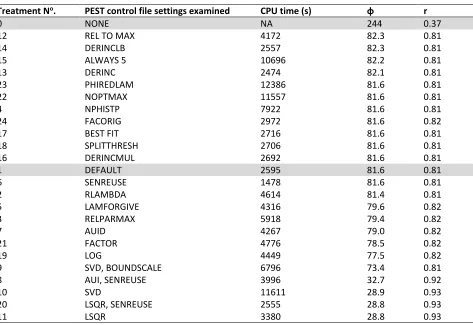
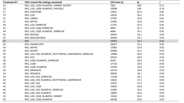
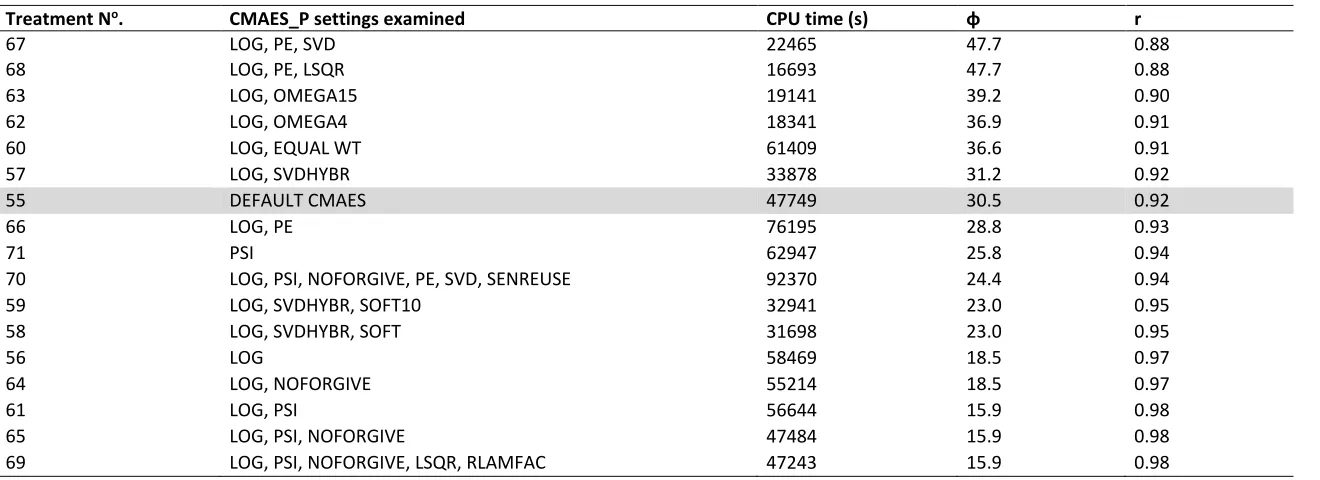
Several techniques for automatic parameterisation are explored using the software PEST. We parameterised the biophysical systems model APSIM with measurements from a maize cropping experiment with the objective of finding algorithms that resulted in the least distance between modelled and measured data (φ) in the shortest possible time. APSIM parameters were optimised using a weighted least-squares approach that minimised the value of φ. Optimisation techniques included the Gauss-Marquardt-Levenberg (GML) algorithm, singular value decomposition (SVD), least squares with QR decomposition (LSQR), Tikhonov regularisation, and covariance matrix adaptation-evolution strategy (CMAES).
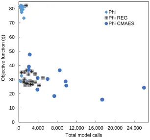
In general, CMAES with log transformed APSIM parameters and larger population size resulted in the lowest φ, but this approach required significantly longer to converge compared with other
optimisation algorithms. Regularisation treatments with log transformed parameters also resulted in
low φ values when combined with SVD or LSQR; LSQR treatments with no regularisation tended to
converge earliest.
In addition to an analysis of several PEST algorithms, this study provides a narrative on how methodologies presented here could be generalised and applied to other models.
Keywords
CPU time; genetic algorithm; inverse modelling; optimization; parameterization; regularization
Software availability
• APSIM version 7.8, programmed in C#.NET and VB.NET, freely available subject to user licencing at http://www.apsim.info/Products/Downloads.aspx
• PEST version 14.2, programmed in FORTRAN, freely available at
http://www.pesthomepage.org/ , Contact address Watermark Numerical Computing, 336 Cliveden Avenue, Corinda 4075, Australia. Telephone 07 3379 1664; Email address [email protected]
Introduction
4
availability of a reproducible calibration methodology helps simplify model calibration documentation in an industry where model documentation has been a long-standing issue (Holzworth et al., 2015; Sexton et al., 2016).
Automated approaches aim to optimise model parameters through programmed directives that assess sequential changes in the objective function (φ), often calculated as the cumulative squared difference between the observed data and corresponding modelled data. Auto-parameterisation methods typically begin with initial parameter sets based on expert knowledge (prior information) and continue to be iteratively upgraded and thus form new parameter vectors until specified
termination criteria are reached. In many algorithms, such criteria are based on the rate of change in
parameters and φ over consecutive iterations. Optimisation problems of this kind may involve
several variables, such that φ is comprised by multiple components. Although automated
approaches for model parameterisation have existed for some time (Lacroix et al., 2002; Samanta and Mackay, 2003; Sequeira et al., 1994), there are few studies that have examined whether auto-parameterisation can be used to calibrate dynamic programs such as APSIM (Keating et al., 2003) (but see notable exceptions by Akponikpè et al. (2010), Chen et al. (2016) and Sexton et al. (2016)). The limitation of past work performing optimisation of agricultural models may be because the objective functions formed by using such models often have discontinuities that make it difficult to use gradient-based minimisation methods (Buis et al., 2011). A common approach, such as that adopted in the crop model OptimiSTICS, is to use the Nelder–Mead simplex algorithm, which is adapted to non-smooth functions because the search of the optimum is not based on the
computation of the function’s gradient. As the Nelder–Mead simplex is a local optimisation method,
OptimiSTICS automatically repeats the minimisation with several different starting parameter values to minimise the risk of converging to a local minimum. However, since this approach requires the user to specify the number of starting points, as well as the starting values in the options file (Buis et al., 2011), it does not guarantee convergence on the global minimum of the response surface. Other approaches, such as generalised likelihood uncertainty estimation (GLUE) (Chisanga et al., 2015; Sexton et al., 2016) and Bayesian parameter estimation (Wallach et al., 2012), yield parameter estimates that are strongly dependent on the choice of likelihood function and the method of combining likelihood values (Seidel et al., 2018). Nonetheless, work by Sexton et al. (2016) showed that both GLUE and Markov Chain Monte Carlo (MCMC) calibrations resulted in accurate simulations of biomass and yield in the crop model APSIM-Sugar.
5
The model-independent Parameter ESTimation software PEST (Doherty, 2016a) has been used successfully with studies of soil biogeochemical models (Necpálová et al., 2015), fractured porous media (Finsterle and Zhang, 2011), remote sensing (Droogers et al., 2010), and tree growth (Gaucherel et al., 2008). Notable advantages of PEST include that (1) the software can generally complete a parameter estimation process with an extremely high level of model run efficiency (Chen et al., 2016), (2) PEST requires little prior knowledge of programming and (3) PEST can be used on a wide range of mathematical models. Further, the freeware is supplied with a number of utility programs that facilitate iterative parameterisation, e.g. multiple rounds of parameterisation via replacement of optimised parameters into PEST control files (PARREP), addition of parameter prior information (ADDREG), differential weighting of observations (PWTADJ) and several other programs that prevent tedious manipulation of PEST control files by users.
PEST optimises model parameters through successive perturbations in response to the difference between modelled and measured data, within which users may implement local or global
optimisers. The default local optimisation scheme uses the Gauss-Levenberg-Marquardt algorithm (Marquardt, 1963), an iterative method that is a hybrid of the Gauss-Newton algorithm and the method of steepest descent. At each step of the iteration, the response surface (φ) is approximated
by the φ value evaluated for the previous parameter set plus the step size multiplied by the Jacobian
matrix (J), which is the derivative of the function with respect to the current parameter set. A critical constant implicit to this process is the value of the damping factor λ, which is adjusted from one iteration to the next. If the sum of the squared deviations between observations and measured values Sis large, λ is reduced, bringing the algorithm closer to the Gauss-Newton algorithm, whereas
if Sis small, λ is increased, such that the algorithm approximates the method of gradient descent
(Marquardt, 1963). When the rate of convergence is low, as would be the case when the gradient of
φ approaches zero, λ is increased in response to reduced curvature of the objective function,
preventing some of the reduction in parameter increment step size as the algorithm converges on the minimum of the response function. The factor used to adjust λ between successive iterations
(RLAMFAC) is one of the variables examined in the present study.
The Gauss-Marquardt-Levenberg (GML) algorithm (hereafter, the ‘default’) in PEST can be used either with or without Tikhonov regularisation. When properly formulated, mathematically regularised inversion has several advantages, including provision for multiple parameters to be calibrated during the matrix inversion (parameterisation) process. Doherty (2016a) indicates that regularised inversion promulgates minimum error variance, and is numerically stable. It does not founder for want of an invertible matrix as the inverse problem is formulated in a way that
guarantees matrix invertibility. Other advantages include the allowance for heterogeneity to emerge in a solution where its existence is supported by data (and suppression of heterogeneity in modelled outcomes where it is not supported by the data), accommodation of model parameter
non-uniqueness, and identification of parameter values that cannot be estimated during inversion (singularity) (Doherty 2016a).
Another optimisation algorithm that can be employed using PEST is covariance matrix evolution strategy (CMAES_P). Unlike the default method in PEST, however, CMAES_P does not require derivatives of model outputs with respect to adjustable parameters in order to enable calibration. Thus it can be employed where model outputs show “numerical granularity” due to model numerical
6
with a pre-defined φ, and updated by a combination of operators (selection, recombination, mutation) to create the next generation (Rouchier et al., 2015). This process is repeated until some stopping criterion is met. The principle of CMAES_P is that each generation of ψ individuals is created following a multivariate normal distribution in which the mean and covariance matrices are adapted after the evaluation of the previous generation (Rouchier et al., 2015). After each
generation, the mean of the distribution is moved towards previously successful individuals, while the covariance matrix is adapted as to favour previously successful mutation steps in the future. The selection is of type (ω, ψ), in that the ω best individuals of the parent generation determine the creation of a number ψ > ω of offsprings, and no individual from the parent generation is kept unto the next one (Rouchier et al., 2015).
Where model derivatives have integrity, the default gradient-based optimisation processes of PEST are likely to be superior to that of CMAES_P (Doherty 2016a). In contrast, where model derivatives do not have integrity, the performance of CMAES_P may be superior to that of the GML algorithm and/or Tikhonov regularisation (Doherty 2016a). Since this study used a multi-component objective function comprised by several diverse biophysical datasets (e.g. grain yield, soil water content,
nitrous oxide emissions etc.), it is likely that the φ surface contains discontinuities, local minima,
noise, and overall is rugged, such that in several locations of the landscape, model derivatives may not have integrity. If this assumption is true, CMAES_P should result in lower overall φ value
compared with PEST’s gradient-based algorithms.
There are several applications where auto-parameterisation approaches could be used in agricultural modelling scenarios. The first is model-intercomparison studies, such as those documented by Rosenzweig et al. (2013), Lampe et al. (2014) and Ehrhardt et al. (2018). In these studies, users were required to calibrate their model of choice using time-series of measured data that were typically measured in the field (Rosenzweig et al., 2013). However, the extent to which anthropogenic elements and/or user predisposition influenced modelled results in such studies is unknown. Another application of auto-parameterisation is to extensive measured datasets, such as that documented by Field et al. (2016), where manual calibration procedures become too tedious due to the number of measured datasets assumed in the calibration. Use of an automated calibration program such as PEST could potentially remove some of the inherent differences in modelled results caused by differences in user parameterisation techniques and/or knowledge, and could automate standardised numerical recipes for model calibration across diverse datasets such as that described by Field et al. (2016).
7
optimal APSIM parameters. The purpose of this study was to identify PEST algorithms (via control file settings) that resulted in the best fit of APSIM simulations to measured data through optimisation of APSIM parameters.
Methods
Experimental data
Data were obtained from experiments conducted at Turin, Italy (44° 53'N, 7° 41'E). Replicated measurements were made for nitrous oxide emissions, above-ground biomass, grain yields,
cumulative crop nitrogen uptake of above-ground biomass, harvest index, and soil water content; all variables except N2O were monitored over three years; N2O was monitored for two years. Four replicated plot measurements were made for each variable except N2O, which had three to nine replicates per treatment (in the present study, we compared all measured variables to simulated values and fitted APSIM to the means of field measurements). Full details of field experiments are provided in Alluvione et al. (2010), Alluvione et al. (2013) and Grignani et al. (2012); only a brief reprise is given here. The data used for this study were part of a larger experiment with multiple treatments that examined agronomic responses and greenhouse gas emissions of maize crops; here we used the urea treatment detailed in Grignani et al. (2012).
The soil at the experimental site was deep, calcareous, and fertile, and had a silty loam texture. The long-term average yearly temperature is 11.9°C, and the long-term average yearly precipitation is 734 mm. The climate type is F (hot temperate climate without dry season, similar to temperate climates), with two main rainfall periods, in spring and autumn (Supplementary information 1).On the day of sowing each year (19 May 2006, 4 June 2007 and 19 May 2008), experimental plots were prepared by mouldboard plowing at 30 cm deep. Seeds of the FAO 500 maize hybrid PR34N43 (Zea Mays L. Pioneer Hi-Bred) were sown 2 cm deep at densities of 7.4 seeds/m2. Mineral fertiliser as urea at a rate equivalent to 130 kg N/ha was applied at sowing each year. Crops were irrigated throughout the growing season according to evapotranspiration requirements (see Supplementary Information 1). Harvesting was conducted on the 22 September 2009, 10 October 2010 and 29 September 2011. Further details of experimental conditions are provided in Grignani et al. (2012). Total biomass and N uptake were assessed by hand-harvesting at dent stage from an area of 15 m2 per plot, with four plot field replicates. Plant samples, separated into grain and shoot/leaves, were oven-dried at 70°C and analysed for N content using a CHN elemental analyser.
Soil NO3−N content was determined by collecting soil samples before sowing, at flowering, and after harvest from three soil layers (0–15, 15–30, 30–60 cm) in all plots and all years. Soil nitrates were extracted by shaking 100 g of moist soil with 300 mL of 1 M KCl solution for 1 h. Subsequently, the samples were filtered and NO3 −N concentration was determined by colorimetry with a continuous flow analyser. Soil moisture was measured on the same dates through weighing c. 100 g of soil before and after oven drying at 105°C.
8
chamber closure and applying proper corrections for fluxes underestimation by the linear model due to the alteration of near-surface concentration gradients (Venterea and Baker, 2008).
Biophysical model for agronomic simulations
APSIM is a biophysical model that simulates the growth and development on a daily time step in response to climate inputs (maximum and minimum daily temperature, solar radiation, rainfall and vapour pressure), soil water, nitrogen, soil organic matter and residue and crop management (Keating et al. 2003). The model is discussed in detail by Keating et al. (2003) and Holzworth et al. (2014). APSIM v7.8 was used to conduct this study. The model was initialised with soil data from Alluvione et al. (2013) (Supplementary information 1); these data included soil water characteristics, organic carbon, pH and soil texture. Crop management conditions in the model were set in line with experimental data described above assuming simulated tillage with discs in the absence of an option to simulate cultivation by mouldboard plows.
As the FAO 500 cultivar used in the field experiments (PR34N43; see Alluvione et al. 2010) was not available in APSIM, a new cultivar was created in the APSIM Maize XML file using the parameters for
the “usa_18leaf” variety provided in the default APSIM cultivars (this variety was selected as it had a
similar thermal time to maturity as that for FAO 500). APSIM parameter files (located in the C:/Program Files/APSIM directory) for the crop (Maize.xml), soil (Soil.xml) and soil organic matter (SurfaceOrganicMatter.xml) were used to establish the cultivar PR34N43 and associated soil
conditions, and later to demark APSIM parameters amendable for modification by PEST (see below).
The ‘ApsimToSim’ executable provided with the default APSIM download package was used to
create an APSIM simulation file (.sim) containing all of the APSIM parameters and management information from both the graphical user interface and XML files mentioned above. Availability of the APSIM .sim file containing all of the parameters in each simulation is a key feature allowing APSIM to be optimised by PEST, as is the ability to run APSIM using command prompt arguments specifying the location of the APSIM model executable (ApsimModel.exe in the MS Windows Program Files directory) and the .sim file to be used in each simulation. The ApsimModel executable allows PEST to run APSIM, read model outputs contained in the APSIM .out files, modify specified parameters in the .sim file, rerun APSIM using the modified .sim file, re-evaluate APSIM outputs, and so on. At the start of the parameterisation process, 115 APSIM parameters were identified as having moderate to significant influence on the magnitude of one or more simulation variables; these APSIM parameters were later used as part of the optimisation process (APSIM has much more than 115 parameters). APSIM parameters optimised by PEST were identified through sensitivity analyses wherein each parameter was individually modified by 10% and the magnitude of change in APSIM outputs observed; any APSIM parameter causing more than 10% change in one or more APSIM outputs was used as a basis for selecting a given APSIM parameter for later optimisation in PEST. Optimised APSIM parameters included those influencing the magnitude and thus temporal variability in soil water (e.g. A_to_evap_fact), soil nitrate or ammonium (e.g. solute_flow_eff), phenology (e.g. tt_enjuv_to_init), biomass (e.g. transp_eff_cf) or grain development (e.g.
9
fractions, such as the root exploration parameter (XF) or the fraction of retained biomass C returned to biomass, we set limits as 1E-9 and 1.0 (PEST does not handle zero value model parameters so instead of zero we set lower bounds to 1E-9). It is important to stress that we chose more
parameters than would be chosen in a typical optimisation process. We did this because we had (1) to ensure that all possible sensitive APSIM parameters were included in the optimisation and (2) to determine whether PEST could optimise so many APSIM parameters simultaneously.
Automated parameterisation protocols for multiple objective functions
The freely available model-independent parameter estimation and uncertainty analysis software PEST (http://www.pesthomepage.org/) was used to conduct the automatic parameterisation processes described here. All optimisation runs were conducted by running either PEST, CMAES_P, or other utility programs in the command prompt. Prior to optimisation, PEST requires four main types of files. These include instruction, template, parameter and control files. Instruction files (extension .ins) were created for APSIM outputs corresponding to yield variables (grain yield, final biomass, grain N concentration, total crop N and total grain N), as well as for soil water, N2O and NO3 in layers 1-3. Instruction files allow PEST to identify which model outputs correspond to
observations, as well as the magnitude to which parameter adjustment influences model outputs. Template files (extension .tpl) were created from APSIM simulation (.sim) files, with hashes (#) for identifying parameters that were amenable for modification by PEST. Parameter files
(extension .par) contain initial APSIM parameter values, parameter scaling (1.0 in all cases) and parameter offsets (0.0 in all cases), as well as precision and decimal point notation of PEST computations (the parameter file for treatment 1 in Table 1. Control files (extension .pst; e.g. see Supplementary information 3) contain all of the information required for PEST to be able to run APSIM, read APSIM output files (.out), alter hash-demarked parameters in the APSIM .sim based on APSIM .out files, then repeat the said process based on the changes in parameters and objective function described below. Control files also contain a number of PEST-specific parameters, each present within defined sections. These include PEST convergence criteria, regularisation constraints, measured field data, parameter transformations, upper and lower bounds for APSIM parameters, parameter groups, prior information equations, specification of APSIM output files, etc. In addition to observations (field measurements) and APSIM parameters subject to modification, the PEST control file also contains so-called ‘parameter groups’ and ‘observation groups’. Parameter groups are variables assigned to common APSIM parameters, e.g. we created the parameter group ‘kl’ that
was assigned to APSIM parameters KL1-KL5 (which specify the maximum rate of water extraction in
each of the five layers of the soil profile). ‘Observation groups’ were groups of field variables (13 in
total); in this study these included biomass, grain yield, harvest index, nitrous oxide emissions, cumulative crop nitrogen uptake, volumetric soil water content in three layers, grain nitrogen content per unit area, grain nitrogen concentration and soil nitrate concentration in three layers. Initial control files were built using the utility program PESTGEN, while instruction, template and control files were checked for errors using the PEST utility programs INSCHEK, TEMPCHEK and PESTCHEK, respectively (see Doherty, 2016b for details on use of these programs). Many of the PEST parameters/allowable settings in the control file were manipulated to determine the best PEST settings required to obtain the lowest possible objective function (i.e. sum of squared weighted residuals) in the fastest possible computational time. These PEST control parameters and settings are now briefly described, however for a detailed description of each PEST setting in each
10 Theory: PEST optimisation algorithms in this study
Three main types of optimisation were employed in this study: the first two included the GML algorithm, the second also included the GML algorithm but also Tikhonov regularisation, and the third included covariance matrix adaptation evolution strategy (PEST implementation abbreviated as CMAES_P). The GML algorithm is a gradient-based optimisation approach, whereas CMAES_P is a
“genetic-type” algorithm that does not employ derivatives to conduct optimisation.
Each of the three main optimisation types were tested with and without one or more minor forms of regularisation. For the purpose of this study, regularisation is a means through which a unique solution is obtained to an inverse problem where the calibration dataset lacks the information to support uniqueness (Doherty, 2016a), i.e. the situation wherein only one combination of model parameters provides the lowest difference between measurements and modelled values. For each of the three main optimisation processes, we examined the effect of adding either singular value decomposition (SVD) or least squares with QR decomposition (LSQR). In contrast to Tikhonov regularisation, which is a major form of regularisation and enables solution of an ill-posed problem by adding information derived from initial parameter estimates (prior information), SVD and LSQR are minor forms of regularisation that remove model parameter combinations from the problem by subdividing the estimated model parameters into two orthogonal subspaces, one comprising the
“calibration solution subspace” and the other the “calibration null space”, the latter of which is
spanned by model parameter combinations that cannot be estimated during an inversion process (C4SF, 2017). In PEST, Tikhonov regularisation can be applied in conjunction with either GML or CMAES_P optimisation and either without or without SVD or LSQR (but SVD and LSQR cannot be combined in any given optimisation).
In this section, we first briefly describe the theoretical background of each of the three optimisation algorithms, then discuss further background to SVD and LSQR. Both optimisation and regularisation algorithms are presented in the context of implementation within the PEST framework.
1. Gauss-Marquardt-Levenberg algorithm (the default)
The GML algorithm used for the default optimisation runs (“estimation mode” in PEST) computes an objective function (φm) based on nonlinear least-squares minimisation between the response surface from the model and the measured data (the ‘m’ subscript denotes measured data). The GML is a gradient-based approach, and as such, may only find local minima. Model parameters are calculated in an iterative fashion as PEST systematically varies model inputs, runs the model, reads the model output, and evaluates the model fit using φm, which represents the weighted least squares difference between observed and simulated values (Doherty and Hunt, 2010). The objective function for the GML algorithm can be expressed as:
φm = [c–Xa]TQm[c - Xa] (1)
where Qm is a diagonal matrix whose ith element qii is the square of the weight wi attached to the ith field measurement, c is a vector of measured values, a is a vector of APSIM parameters to be estimated, X is a matrix of APSIM outputs based on parameter vector a and collocated with the observations in c, and T indicates matrix transpose. Following Lin (2005), the parameter vector a is updated on iteration j + 1 using:
11
observations in the calibration dataset to the adjustable model parameters aj), ρ is a PEST parameter between 0 and 1 which is chosen so that φm(aj+1) < φm(aj), B is a diagonal matrix with elements taken from JTJ, and λ (the Marquardt lambda) is computed numerically during each iteration.
Equation (1) can be alternatively expressed as
φm =
∑
𝑛𝑖=1[𝑤𝑖𝑟𝑖]2(3)
Where 𝑟𝑖 (the ith residual) is the difference between the modelled and measured value for the ith measured variable and 𝑤𝑖 is the corresponding weight matrix attributed to the ith residual. n represents the total number of observation groups. Thus, in this study, the 13 components of φm included grain yield, biomass, harvest index, grain N concentration, cumulative crop N uptake, grain N content, volumetric soil water content in three layers, soil nitrate concentration in three layers and soil nitrous oxide emissions. For treatments 1-24, each weight 𝑤𝑖 was assigned using the PEST utility program PWTADJ2 such that weights were inversely proportional to the standard deviation of
each ‘observation group’ in the PEST control file (there were 13 observation groups). Weights were
uniformly assigned within observation groups but differentially across observation groups. Weighting in this way defends the inversion process against one or more observation groups with high standard deviation dominating the value of φm. Weighting applied in all treatments is shown in Supplementary information 5.
At the start of each iteration, the relationship between the best model parameters and model outputs is linearised using a Taylor-series expansion. The finite-difference method is used to compute the Jacobian matrix (Necpálová et al., 2015). The linearised solution is then solved for the updated model parameter set using the GML algorithm, and the new φm is calculated as defined above. The model parameter changes and value of φm are compared with those of the previous iteration to determine if another iteration is justified. If it is, the entire process is repeated; if not, the parameter estimation process terminates (Doherty, 2016a).
In PEST, the real variable RLAMBDA1 is the initial value of λ (Eqn. 2). In general, the value of λ should
decrease as the number of iterations increases. The effect of RLAMBDA1 was tested because the initial value may have an impact on the rate of convergence of the algorithm and the final value of the objective function. Doherty (2016a) indicates that ill-posed problems are more likely to result in singularity in matrix inversion (singularity prevents matrix inversion and thus derivation of optimal parameter vectors). For such problems, increasing the value of RLAMBDA1 to 10 (from the default of 5) and setting the value of RLAMFAC to -3 (the factor by which PEST adjusts λ as it tests different
values of this variable for their efficacy in lowering φ). By setting RLAMFAC to -3, PEST adjusts λ during each iteration of the inversion process so that λ can achieve a value of 1.0 with three
adjustments. This allows rapid adjustment of λ if local parameter insensitivity promulgates sudden problem ill-posedness (Doherty, 2016a).
2. Gauss-Marquardt-Levenberg algorithm with Tikhonov regularisation
The second main optimisation algorithm employed in this study also used the GML algorithm, but included Tikhonov regularisation (treatments 25-54). Mathematical “regularisation” is the process of adding information into an optimisation search to solve an ill-posed problem and to prevent over-fitting. To conduct optimisation runs using Tikhonov regularisation, PEST must be run in
“regularisation” mode, wherein PEST defines two objective functions instead of only one defined in
12
measurement objective function, designated φm, and the regularisation objective function,
designated φr. This constitutes a weighted least-squares measure of the discrepancies between the
model parameters and their preferred conditions:
φr = [d–Za]T Qr[d - Za] (4)
where φr is a diagonal matrix of the squares of weights assigned to the various “regularisation
observations” which comprise vector d. The relationships between the regularisation observations in
d and their model-generated counterparts (calculated from model parameter vector a) are encapsulated in matrix Z (Doherty, 2016a).
To assign every APSIM parameter with a preferred value equal to its initial value, the ADDREG1 utility program described in Doherty (2016b) was used. The ADDREG1 program adds a series of prior information equations to the PEST control file that are assigned to PEST parameter groups beginning
with “regul_” in the “prior information section” (see Supplementary information 3). Collectively, the
addition of prior information equations using ADDREG1 comprises a Tikhonov regularisation scheme (Doherty, 2016b). In essence, prior information equations constitute a set of observations which pertain directly to the model parameters themselves. As such, they comprise part of the calibration dataset which assists in the estimation of APSIM parameters. Using ADDREG1, one linear prior equation is added for each APSIM parameter cited in the control file. In each prior equation, the APSIM parameter is set equal to its initial value (or the log of its initial value if the APSIM parameter is transformed). Similar to individual observations in the PEST control file, weights must be assigned to each prior equation; these weights are multiplied internally by a regularisation weight factor (μ)
before formulation of an overall φ during each iteration of the inversion process (Eqn. 6 below).
Treatments 25-54 had 115 prior information equations and 69 observation groups (56 of which were associated with prior information; e.g. see Supplementary information 3). All prior information equations were assigned a weight of 1.0 (the default). Setting the PEST variable IREGADJ to 1.0 allows PEST to vary the regularisation weights between groups, thus complementing the information density of the calibration dataset (Doherty, 2016b).
By way of example of prior information, for the APSIM soil nitrogen denitrification parameter we created the PEST parameter ‘dnitcof’ and a corresponding regularisation group parameter called
‘regul_dnitco’ (all APSIM parameters optimised by PEST must be represented by corresponding PEST
parameter names less than or equal to 12 characters in length). The prior information equation thus created using ADDREG1 was:
log10(dnitcof) = -2.97 (5)
where the log was introduced as the PEST parameter denitcof for this example was log transformed prior to the inversion process (see Supplementary information 3) and -2.97 represents the log of the initial dnitcof value (1.05E-03). Throughout the optimisation process, the extent to which dnitcof differs from 1.05E-3 causes a non-zero residual, and the value of φr in Eqn. 5 becomes non-zero. To prevent over-fitting, the user is required to provide a target measurement objective function
(φtm). This is the value of PHIMLIM shown in Tables 1-4 (set to 1.00E-10 in treatments 25-54). PEST
attempts to minimise the value of φr subject to the constraint provided by φtm. In solving this
constrained minimisation problem, PEST applies a global multiplier to all weights that are ascribed to prior information equations (Doherty 2016a). During each iteration of the inversion process, PEST minimises the total objective function:
13
where μ is the regularisation weighting factor. During each iteration, PEST computes the optimal value of μ. Under the linearity assumption used to compute the Jacobian matrix, this is the value of μ
that results in a model parameter upgrade vector for which φm is reduced to a value as close as
possible to φmt. When PEST is not able to lower φm to φmt, it accepts the upgraded model parameters
and proceeds to the next iteration. However, if PEST does succeed in lowering φm to an acceptable
level, it then attempts to lower φr while maintaining φm below this acceptable level. This acceptable
level is the variable PHIMACCEPT and should be set slightly higher than φmt (the default
PHIMACCEPT value is 1.05E-10).
The PEST parameter FRACPHIM shown in Tables 1-4 represents the new value for φtm calculated at the beginning of every iteration; this value is calculated as the current value of φm times FRACPHIM, or the current value of FRACPHIM, whichever is greater. FRACPHIM was set to 0.1 for treatment 25. WFINIT, WFMIN and WFMAX are the initial, minimum and maximum permissible regularisation weight factors, respectively. PEST parameter WFFAC defines the multiplier used to adjust the regularisation weight factor such that the value of φm equals that of φml, whilst PEST parameter WFTOL defines the maximum allowed difference between two successive weighting factors (Doherty 2016a). The variable IREGADJ is used to adjust the weighting factor within regulation groups. When it is set to 1, PEST multiplies the weights pertaining to all members of each regularisation group by a group-specific factor. This factor is chosen so that the total
composite sensitivities of all regularisation groups are the same. It is important to note, however, that relative weighting within each observation group remains unchanged when IREGADJ equals 1.0 (Doherty 2016a).
3. Covariance matrix adaptation-evolution strategy
The PEST control files for the GML algorithms were also compatible for use with the third main algorithm employed in this study: covariance matrix adaptation-evolution strategy (PEST
implementation abbreviated CMAES_P). In contrast to the GML algorithm, CMAES_P does not apply gradient-based methods, and thus is theoretically capable of finding the global minimum of the search space. In CMAES_P, a population of new search points (ψ≥ 2) is generated by sampling a multivariate normal distribution. The basic equation for sampling the search points for generation number g reads:
xk(g + 1)~m(g)+σ(g)ѵ(0, C(g)) for k = 1, … , ψ (7) where ~ denotes the same distribution on the right and left hand sides, ѵ(0, C(g)) is a multivariate
normal distribution with zero mean and covariance matrix of the search distribution C(g),x k(g + 1) represents the kth offspring (individuals, search points) from generation g + 1, m(g) represents the
weighted average value of the search distribution of ω selected parents (ω < ψ) at generation g, and σ(g)is the overall standard deviation (step-size). The number of generations g depends on CMAES_P
termination criteria that are prescribed by the user. Further details of CMAES and supporting theoretical background are described in Hansen (2016).
14
information, and whether or not model parameters causing model run failures should be weighted lower than other model parameter vectors.
For CMAES_P, weights corresponding to ω model parameter sets can be assigned as “super-linear”,
“linear”, or “equal”. In the first two cases, greater weight is given to model parameters that give rise
to lower φ values, this often leading to faster reduction of the objective function. Since the first two
cases tend to elicit similar responses in model optimisation runs, this study only examined
“superlinear” and “equal” weighting (the latter in treatment 60). Once a new average set of model
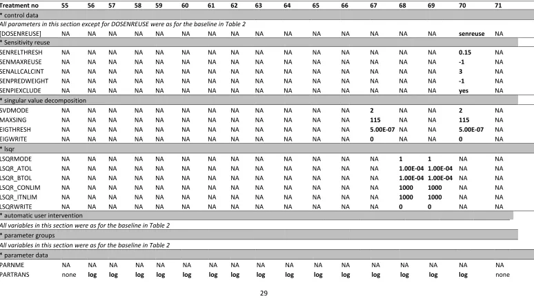
parameter values has been computed in this fashion, the next iteration begins. Because random model parameter realisations are generated to be symmetrical about this mean, there is a tendency for the objective function to fall as iterations proceed (Doherty 2016a). A caveat of CMAES_P is run time burden in optimisation runs that include multiple model parameters. In this study, CMAES_P would not allow simultaneous optimisation of 115 APSIM parameters, so the number of optimised parameters was reduced from 115 in GML optimisation runs (treatments 1-54), to 84 in treatments performed by CMAES_P (55-71). Accordingly, the number of PEST parameter groups in CMAES_P treatments was reduced to 39. The 31 APSIM parameters removed from the GML control files in preparation for the CMAES_P runs were chosen according to their sensitivity. These APSIM parameters were identified from the PEST “.sen” files that were produced after each GML optimisation run (APSIM parameter sensitivity was consistent regardless of treatment applied). Inspection of .sen files showed that insensitive APSIM parameters were not modified by PEST during GML or Tikhonov regularisation runs. Thus, it is likely that the fewer parameters contained in the CMAES_P treatments had little effect on the final degree of fit achieved. APSIM parameters optimised using CMAES_P are shown in Supplementary Information 2.
At the CMAES_P prompt, users must select whether “soft” or “hard” hybridisation takes place.
“Soft” hybridisation replaces the best of the currently-selected ψ parameters (these forming part of
the m + 1 member parameter set on which SVD analysis was based) with the SVD-computed parameter set if the value of φ achieved through SVD yields the lowest φ to date. If the “hard”
option is selected, parameter set replacement is undertaken if the SVD-computed parameter set
leads to a lower φ than that computed only on the basis of the current ψ parameter sets (Doherty
2016a).
4. Minor regularisation methods: singular value decomposition (SVD) and least-squares with QR decomposition (LSQR)
In PEST either singular value decomposition (SVD) or LSQR (Least Squares with QR decomposition) can be combined with any other optimisation algorithm. Both methods were originally developed for the inversion of ill-conditioned matrices (Lanczos, 1961; Paige and Saunders, 1982). In contrast to the analytical approach afforded by SVD, LSQR is an iterative numerical approach designed for inversion of large matrices. Although LSQR generally allows faster convergence, it is an
approximate measure and thus may not result in φ values that are as low as those obtained using SVD. Hence, we investigated the influence of both SVD and LSQR on the value of φ and
computational time for each of the three main algorithms described above.
SVD is a form of matrix factorisation into rotational and scaling matrices, enabling tractability to the solution of ordinary least-squares problems in matrix inversion by preventing matrix
15
on a stability criterion. SVD transforms the original model parameters into linear combinations (i.e., eigenvectors), determines which are most sensitive (James and John, 2005; Moore and Doherty, 2006), and truncates the transformed normal equations matrix, reducing the number of estimated parameters to maintain numerical stability and maximum reasonableness (Aster et al., 2013). The resulting regularised inversion process will not include parameters that are
unidentifiable with the available data. When correlated parameters are included in the inversion, the SVD-based regression finds the maximum likelihood combination of the parameters that is consistent with the observations (Necpálová et al., 2015). In all SVD treatments in this study, the PEST variable SVDMODE was set to 2, such that PEST undertook singular value decomposition of the Q1/2J matrix, where Q is a weighting matrix and J represents the Jacobian matrix described
above.
The LSQR algorithm (Least Squares with QR decomposition) represents another mechanism that can be used to solve inverse problems (Paige and Saunders, 1982). LSQR attempts to subdivide
parameter space into orthogonal null and solution spaces, and then restricts solution of the inverse problem to the latter space (Paige and Saunders, 1982). Because LSQR facilitates matrix sparsity and compartmentalisation of the solution into a matrix subspace (rather than attempting to linearise the entire solution as conducted by SVD), LSQR tends to converge much faster than SVD (Lin et al., 2016).
Treatments conducted in this study
Seventy-one treatments were conducted. These examined various PEST control file settings for each of the optimisation algorithms and regularisation techniques presented above. Table 1 presents a brief description of the PEST parameters examined in this study, while Tables 2-4 show the values of PEST parameters compared with their default values. Treatments 1-24 describe PEST optimisation runs conducted in the ‘estimation’ mode (using the GML theorem), Treatments 24-54 were
conducted in ‘regularisation’ mode and thus used the GML algorithm with Tikhonov regularisation,
while treatments 55-71 were conducted using CMAES_P (Table 4). Descriptions in Table 1 provide a minimal level of background required to enable understanding of the concepts used in this study; more detail regarding PEST parameters and theory underlying each treatment is shown in
Supplementary information 4, Doherty (2016a) and Doherty (2016b).
Treatment 0 contained only management and soil information measured at the site; no
parameterisation was conducted for this treatment. PEST was used to compute φ for this treatment
using the control file from treatment 1 (see below) but with the number of optimisation runs set to zero (using PEST parameter NOPTMAX in the control file). This treatment was not judged as the baseline because the maize hybrid used in the field trials was not available in APSIM; as such, part of the calibration process in all treatments involved optimising parameters for the new hybrid in APSIM.
16
others. Weighting applied by PWTADJ2 was retained for all treatments except treatments 52 and 53, which were designed to examine the effect of observation group weighting. Treatment 52 adopted the optimised parameters from one of the better performing treatments (treatment 43), then increased weighting applied to the N2O group, since results showed that relative contribution to φ
from this group was large. The weighting applied to all N2O observations was increased from 4.203
(as for previous treatments) to 20, with the rationale that PEST would thus “focus” on reducing the
error between modelled data and measurements of this observation group. Similar to treatment 52, treatment 53 reused the optimised parameters resulting from treatment 43. The PWTADJ1 utility program provided with PEST was used to re-adjust the weighting applied to all datasets, such that the total contribution of all datasets to φ was 10. A summary of observation group weighting for all treatments is provided in Supplementary information 5.
For treatments 1-54, 115 APSIM parameters were demarked within the PEST template file by hashes (#) along with a user-assigned parameter name. Corresponding upper and lower bounds were specified for each of these parameters in the PEST control file and were not altered between treatments. For all treatments in Tables 2 and 3, there were 117 field measurements, 56 parameter groups, 0 prior equations, and 13 observation groups in the PEST control files.
To identify sensitive PEST parameters in the control file, groups of only two or three PEST parameters were modified from the baseline file on a piecemeal basis to test the effect of
alternative setting groups on the value of the objective function and total run time. However, some of the parameters in the PEST control file required more than one PEST parameter to be modified (e.g. in the ‘parameter groups’ section, the use of split derivatives required three settings to be simultaneously modified from the baseline file). After key PEST control file parameters causing a significant effect on optimisation time or the objective function deviation from the default value (or both) were identified, combinations of up to five PEST parameters in the control file were modified and tested to determine whether the combined effect of sensitive PEST parameters on total model calls and objective function value was additive or otherwise. Thus, treatments that employed Tikhonov regularisation (Table 3) were constructed based on previous runs without regularisation that reduced either φ or the total number of model calls. It should also be noted that although this study explores and extensive number of PEST parameter combinations, not all possible parameter combinations were explored.
Model evaluation criteria
17
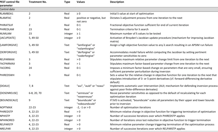
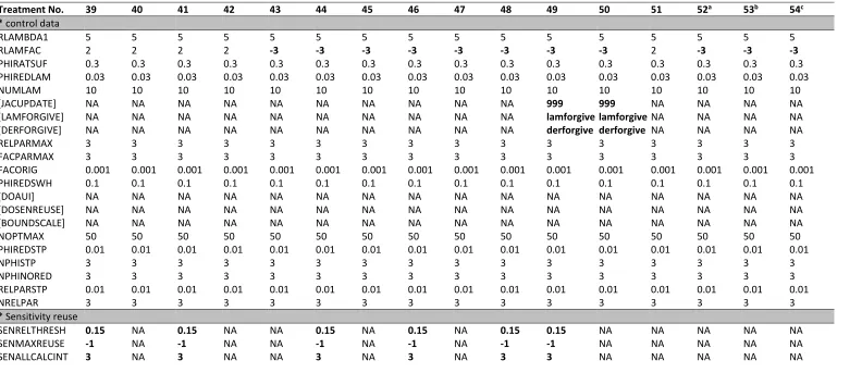
Table 1 Treatments used to examine PEST control file parameters (table layout follows PEST control file). Parameter descriptions are summarised from Doherty et al (2016a). Variables in square brackets are optional in PEST.
PEST control file parameter
Treatment No. Type Values Description
Control data
RLAMBDA1 2 Real ≥ 0 Initial λ value at start of optimisation
RLAMFAC 2 Real positive or negative, but
not zero
Dictates λ adjustment process from one iteration to the next
PHIRATSUF 2 Real 0-1 Fractional objective function sufficient for end of current iteration
PHIREDLAM 23 Real 0-1 Termination criteria for λ search
NUMLAM 23 integer ≥ 1 Maximum number of λ values to be tested
[JACUPDATE] 5, 49-50 integer ≥ 0 Activation of Broyden's Jacobian update procedure (mechanism for improving Jacobian
matrix)
[LAMFORGIVE] 5, 49-50 Text "lamforgive" or
"nolamforgive"
Assign a high objective function value to any λ search resulting in an APSIM run failure
[DERFORGIVE] 5, 49-50 Text "derforgive" or
"noderforgive"
Accommodates model failure whilst computing the Jacobian by setting pertinent parameter sensitivities to zero
RELPARMAX 3 Real > 0 Stipulates maximum relative parameter change limit from one iteration to the next
FACPARMAX 3 Real > 1 Stipulates maximum factor-based parameter change from one iteration to the next
FACORIG 24 Real 0-1 Imposes a minimum factor-based change on parameters that are very small, ensuring
sufficient parameter perturbation during inversion
PHIREDSWH 3 Real 0-1 Sets a value for the relative change in objective function for one iteration to the next that
stipulates introduction of 3- or 5-point derivatives (cf. forward-differencing derivative default)
[DOAUI] 7, 8 Text "aui", "auid" or "noaui" Implements automatic user intervention (AUI; mechanism for defending inversion process against poor finite-difference derivates)
[DOSENREUSE] 6-8, 20, 70 Text "senreuse" or
"nosenreuse"
Reuse parameter sensitivities as opposed to the default of recalculating for each optimisation iteration
[BOUNDSCALE] 9 Text "boundscale" or
"noboundscale"
If SVD is activated, "boundscale" scales all parameters by their upper and lower bounds prior to inversion
NOPTMAX 22-23 integer -2, -1 or > 0 Number of optimisation iterations
PHIREDSTP 4, 22-23 Real > 0 Minimum relative change in objective function for triggering termination of optimisation
NPHISTP 4, 22-23 integer > 0 Number of successive iterations over which PHIREDSTP applies
NPHINORED 4, 22-23 integer > 0 Number of iterations since last reduction in objective function to trigger termination
RELPARSTP 4, 22-23 Real > 0 Minimum relative parameter change triggering termination of the optimisation process
18 Sensitivity reuse
SENRELTHRESH 6-8, 20, 38-39, 41, 44, 46, 48-49, 70
Real 0-1 Relative parameter sensitivity below which sensitivity reuse is activated for a parameter
SENMAXREUSE 6-8, 20, 38-39, 41, 44, 46, 48-49, 70
integer ≥ 1 Maximum number of reused sensitivities per iteration
SENALLCALCINT 6-8, 20, 38-39, 41, 44, 46, 48-49, 70
integer > 1 Iteration interval at which all sensitivities are recalculated
SENPREDWEIGHT 6-8, 20, 38-39, 41, 44, 46, 48-49, 70
Real any number Weight to assign to prediction in computation of composite parameter sensitivities to determine sensitivity reuse
SENPIEXCLUDE 6-8, 20, 38-39, 41, 44, 46, 48-49, 70
Text "yes" or "no" Include/exclude prior information when computing composite parameter sensitivities to determine sensitivity reuse
Singular value decomposition
SVDMODE 9-10, 35, 39, 40, 45-46,
49-50, 67, 70
integer 0 or 1 If SVDMODE is set to 1, activates truncated SVD for solution of inverse problem
MAXSING 9-10, 35, 39, 40, 45-46,
49-50, 67, 70
integer > 0 Number of singular values before truncation
EIGTHRESH 9-10, 35, 39, 40, 45-46,
49-50, 67, 70
Real ≥ 0 and < 1 Ratio of the lowest to the highest eigenvalue of the (JtQJ + λI) matrix at which singular value truncation occurs (see text in Methods)
EIGWRITE 9-10, 35, 39, 40, 45-46,
49-50, 67, 70
integer 0 or 1 Determines whether SVD file resulting from PEST inversion process is written to text file
LSQR
LSQRMODE 11, 20, 36, 41-44, 47-48,
52-54, 68-69
integer 0 or 1 Activates LSQR solution of the inversion problem
LSQR_ATOL 11, 20, 36, 41-44, 47-48,
52-54, 68-69
Real ≥ 0 Estimate of the relative error in the data defining the Q1/2J matrix used in LSQR (see text in Methods)
LSQR_BTOL 11, 20, 36, 41-44, 47-48,
52-54, 68-69
Real ≥ 0 Estimate of the relative error in the data defining the parameter vector a in Eqn. 1
LSQR_CONLIM 11, 20, 36, 41-44, 47-48, 52-54, 68-69
Real ≥ 0 Upper limit of the matrix condition number during the inversion process (higher condition
numbers indicate ill-posedness) LSQR_ITNLIM 11, 20, 36, 41-44, 47-48,
52-54, 68-69
integer > 0 Upper limit of the number of iterations permitted when LSQR is employed
LSQRWRITE 11, 20, 36, 41-44, 47-48,
52-54, 68-69
integer 0 or 1 Writes output from the LSQR solver to an output file
Automatic user intervention
MAXAUI 7-8 integer ≥ 0 Maximum number of automatic user interventions per optimisation iteration
AUISTARTOPT 7-8 integer ≥ 1 Optimisation iteration at which to commence automatic user intervention
NOAUIPHIRAT 7-8 Real 0-1 Relative objective function reduction threshold triggering automatic user intervention
19
AUISENSRAT 7-8 Real > 1 Composite parameter sensitivity ratio triggering automatic user intervention
AUIHOLDMAXCHG 7-8 integer 0 or 1 When implemented, instructs PEST to hold specific parameters based on their relative
change during previous optimisation iterations
AUINUMFREE 7-8 integer > 0 Cease automatic user intervention if the number of adjustable parameters has been
reduced to AUINUMFREE
AUIPHIRATSUF 7-8 Real 0-1 Ratio of objective function computed using AUI to that computed without AUI. If
AUIRATSUF is less than this value, implementation of automatic user intervention is terminated
AUIPHIRATACCEPT 7-8 Real 0-1 Relative objective function reduction threshold for acceptance of automatic-user
intervention-calculated parameters
NAUINOACCEPT 7-8 integer > 0 Number of iterations since accepting previous parameter change that triggers termination
of automatic user intervention Parameter groups
INCTYP 12 Text "relative", "absolute",
"rel_to_max"
Method by which parameter increments are calculated
DERINC 13 Real > 0 Absolute or relative parameter increment (added or multiplied to existing parameters
depending on the value of INCTYP)
DERINCLB 14 Real ≥ 0 Absolute lower bound of relative parameter increment
FORCEN 15 Text "switch", "always_5" Determines when higher order derivatives are undertaken for each parameter group
(always_5 = five-point derivatives are used, switch = start by using forward difference derivatives then switch to three-point derivatives for all parameter group members on the first occasion that the relative reduction in the objective function between iterations is less than the value of PHIREDSWH)
DERINCMUL 16 Real > 0 Derivative increment multiplier when undertaking derivatives using methods other than
the default forward-differencing method
DERMTHD 15, 17 Text "parabolic", "minvar" or
"best_fit"
Method used to calculate derivatives ("min_var" means minimum error variance; must be implemented with "always_5", "best_fit" is a regression approach implemented with "switch")
[SPLITTHRESH] 18, 49-50 Real > 0 (0 = deactivation of
split slope analysis)
Slope threshold for split slope analysis (an option for mitigating effects of poor model numerical performance on PEST performance wherein segmented analysis is used to compute the change in each parameter)
[SPLITRELDIFF] 18, 49-50 Real > 0 Relative slope difference threshold allowing implementation of split slope analysis
[SPLITACTION] 18, 49-50 Text "smaller" The slope segment with higher absolute value is rejected, and the derivative is taken as the
slope of the segment with lesser absolute slope Parameter data
PARTRANS 19, 37-46, 49, 52-54, 56-70,
72
Text "log" or "none" Parameter transformation prior to inversion ("log" = log to the base 10)
PARCHGLIM 19, 21, 37-46, 49, 52-54,
56-70, 72
20 Regularisation
PHIMLIM 66-71 Real > 0 Target measurement objective function (see text in Methods)
PHIMACCEPT 26, 66-71 Real > PHIMLIM Acceptable measurement objective function (see text in Methods)
[FRACPHIM] 27, 66-71 Real ≥ 0 (< 1) Sets target measurement objective function at this fraction of current measurement
objective function
[MEMSAVE] 28 Text "memsave" or
"nomemsave"
Activates conservation of memory at cost of execution speed and quantity of model output
WFINIT 29, 66-71 Real > 0 Initial regularisation weight factor (see text in Methods)
WFMIN 66-71 Real > 0 Minimum regularisation weight factor
WFMAX 66-71 Real > WFMIN Maximum regularisation weight factor
[LINREG] 51 Text "linreg" or "nolinreg" Instructs PEST that regularisation constraints are linear or nonlinear, respectively
[REGCONTINUE] 32 Text "continue" or
"nocontinue"
Instructs PEST to continue minimising regularisation objective function even if measurement objective function is less than PHIMLIM (see text in Methods)
WFFAC 30, 66-71 Real > 1 Regularisation weight factor adjustment (see text in methods)
WFTOL 31, 66-71 Real > 0 Convergence criterion for regularisation weight factor calculated during each iteration
IREGADJ 33, 34, 66-71 integer 1, 2 or 4 Instructs PEST to perform inter-regularisation group weight factor adjustment, or to
compute new relative weights for regularisation observations and prior information equations (see text in Methods)
[NOPTREGADJ] 34 integer ≥ 1 The number of consecutive optimisation iterations stipulating recalculation of
regularisation weight factor
[REGWEIGHTRAT] 34 Real ≥ 1 The ratio of the highest to lowest regularisation weight (see text in Methods)
CMAES_P
Population size (ψ) 61, 65, 69-72 integer [4 + 3 × ln(n)] Number of random realisations of n-dimensional parameter vectors generated during each
iteration of CMAES_P (n = the number of parameters being estimated)
Number of parents (ω) 62-63 integer ψ/2 Number of objective function values used to calculate m in Eqn. 7 for the next iteration.
Default value is half the population size. Recombination weights 60 Text "linear", "superlinear" or
"equal"
Weighting given to the lowest objective function values in forming m (Eqn. 7) for the next iteration
SVD-hybridisation 57-59 Text "soft" or "hard" Uses all or a subset of the current iteration ψ parameter sets to compute approximate
SVDs (see text in Methods) No. singular value trial
thresholds
57-59 integer ≥ 1 Determines level of single value truncation if SVD-hybridisation is employed
Forgive model run failure
21
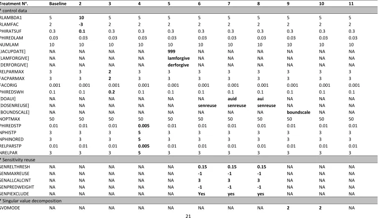
Table 2 Data from PEST control files used to conduct optimisation with the GML algorithm. All optimisation runs were performed using ‘estimation’ mode in PEST, with 115 parameters, 56 parameter groups, 13 observation groups and no prior equations. Parameters shown in bold indicate variation from the baseline file (treatment 1). PEST control settings in the first column are described in the methods, and parameters in square brackets [] indicate optional use in the PEST control file. Each control file section is identified with an asterisk. NA = Not Applicable.
Treatment No. Baseline 2 3 4 5 6 7 8 9 10 11
* control data
RLAMBDA1 5 10 5 5 5 5 5 5 5 5 5
RLAMFAC 2 -3 2 2 2 2 2 2 2 2 2
PHIRATSUF 0.3 0.1 0.3 0.3 0.3 0.3 0.3 0.3 0.3 0.3 0.3
PHIREDLAM 0.03 0.03 0.03 0.03 0.03 0.03 0.03 0.03 0.03 0.03 0.03
NUMLAM 10 10 10 10 10 10 10 10 10 10 10
[JACUPDATE] NA NA NA NA 999 NA NA NA NA NA NA
[LAMFORGIVE] NA NA NA NA lamforgive NA NA NA NA NA NA
[DERFORGIVE] NA NA NA NA derforgive NA NA NA NA NA NA
RELPARMAX 3 3 2 3 3 3 3 3 3 3 3
FACPARMAX 3 3 2 3 3 3 3 3 3 3 3
FACORIG 0.001 0.001 0.001 0.001 0.001 0.001 0.001 0.001 0.001 0.001 0.001
PHIREDSWH 0.1 0.1 0.2 0.1 0.1 0.1 0.1 0.1 0.1 0.1 0.1
[DOAUI] NA NA NA NA NA NA auid aui NA NA NA
[DOSENREUSE] NA NA NA NA NA senreuse senreuse senreuse NA NA NA
[BOUNDSCALE] NA NA NA NA NA NA NA NA boundscale NA NA
NOPTMAX 50 50 50 50 50 50 50 50 50 50 50
PHIREDSTP 0.01 0.01 0.01 0.005 0.01 0.01 0.01 0.01 0.01 0.01 0.01
NPHISTP 3 3 3 5 3 3 3 3 3 3 3
NPHINORED 3 3 3 5 3 3 3 3 3 3 3
RELPARSTP 0.01 0.01 0.01 0.005 0.01 0.01 0.01 0.01 0.01 0.01 0.01
NRELPAR 3 3 3 5 3 3 3 3 3 3 3
* Sensitivity reuse
SENRELTHRESH NA NA NA NA NA 0.15 0.15 0.15 NA NA NA
SENMAXREUSE NA NA NA NA NA -1 -1 -1 NA NA NA
SENALLCALCINT NA NA NA NA NA 3 3 3 NA NA NA
SENPREDWEIGHT NA NA NA NA NA -1 -1 -1 NA NA NA
SENPIEXCLUDE NA NA NA NA NA Yes yes yes NA NA NA
* Singular value decomposition
22
MAXSING NA NA NA NA NA NA NA NA 115 115 NA
EIGTHRESH NA NA NA NA NA NA NA NA 5E-07 5E-07 NA
EIGWRITE NA NA NA NA NA NA NA NA 0 0 NA
* lsqr
LSQRMODE NA NA NA NA NA NA NA NA NA NA 1
LSQR_ATOL NA NA NA NA NA NA NA NA NA NA 0.0001
LSQR_BTOL NA NA NA NA NA NA NA NA NA NA 0.0001
LSQR_CONLIM NA NA NA NA NA NA NA NA NA NA 1000
LSQR_ITNLIM NA NA NA NA NA NA NA NA NA NA 1000
LSQRWRITE NA NA NA NA NA NA NA NA NA NA 0
* automatic user intervention
MAXAUI NA NA NA NA NA NA 87 87 NA NA NA
AUISTARTOPT NA NA NA NA NA NA 1 1 NA NA NA
NOAUIPHIRAT NA NA NA NA NA NA 0.9 0.5 NA NA NA
AUIRESTITN NA NA NA NA NA NA 0 0 NA NA NA
AUISENSRAT NA NA NA NA NA NA 5 10 NA NA NA
AUIHOLDMAXCHG NA NA NA NA NA NA 0 0 NA NA NA
AUINUMFREE NA NA NA NA NA NA 3 3 NA NA NA
AUIPHIRATSUF NA NA NA NA NA NA 0.8 0.4 NA NA NA
AUIPHIRATACCEPT NA NA NA NA NA NA 0.99 0.8 NA NA NA
NAUINOACCEPT NA NA NA NA NA NA 30 30 NA NA NA
* parameter groups
INCTYP relative relative relative relative relative relative relative relative relative relative relative
DERINC 0.01 0.01 0.01 0.01 0.01 0.01 0.01 0.01 0.01 0.01 0.01
DERINCLB 0 0 0 0 0 0 0 0 0 0 0
FORCEN switch switch switch switch switch switch switch switch switch switch switch
DERINCMUL 2 2 2 2 2 2 2 2 2 2 2
DERMTHD parabolic parabolic parabolic parabolic parabolic parabolic parabolic parabolic parabolic parabolic parabolic
[SPLITTHRESH NA NA NA NA NA NA NA NA NA NA NA
SPLITRELDIFF NA NA NA NA NA NA NA NA NA NA NA
SPLITACTION] NA NA NA NA NA NA NA NA NA NA NA
* parameter data
PARTRANS none none none none none None none none none none none
23
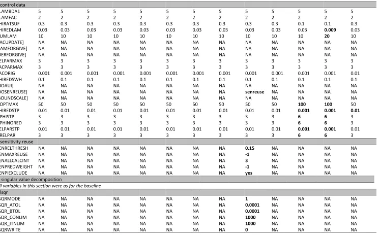
Table 2 Continued.
Treatment No. 12 13 14 15 16 17 18 19 20 21 22 23 24
* control data
RLAMBDA1 5 5 5 5 5 5 5 5 5 5 5 5 5
RLAMFAC 2 2 2 2 2 2 2 2 2 2 2 2 2
PHIRATSUF 0.3 0.3 0.3 0.3 0.3 0.3 0.3 0.3 0.3 0.3 0.1 0.1 0.3
PHIREDLAM 0.03 0.03 0.03 0.03 0.03 0.03 0.03 0.03 0.03 0.03 0.03 0.009 0.03
NUMLAM 10 10 10 10 10 10 10 10 10 10 10 20 10
[JACUPDATE] NA NA NA NA NA NA NA NA NA NA NA NA NA
[LAMFORGIVE] NA NA NA NA NA NA NA NA NA NA NA NA NA
[DERFORGIVE] NA NA NA NA NA NA NA NA NA NA NA NA NA
RELPARMAX 3 3 3 3 3 3 3 3 3 3 3 3 3
FACPARMAX 3 3 3 3 3 3 3 3 3 3 3 3 3
FACORIG 0.001 0.001 0.001 0.001 0.001 0.001 0.001 0.001 0.001 0.001 0.001 0.001 0.01
PHIREDSWH 0.1 0.1 0.1 0.1 0.1 0.1 0.1 0.1 0.1 0.1 0.1 0.1 0.1
[DOAUI] NA NA NA NA NA NA NA NA NA NA NA NA NA
[DOSENREUSE] NA NA NA NA NA NA NA NA senreuse NA NA NA NA
[BOUNDSCALE] NA NA NA NA NA NA NA NA NA NA NA NA NA
NOPTMAX 50 50 50 50 50 50 50 50 50 50 100 100 50
PHIREDSTP 0.01 0.01 0.01 0.01 0.01 0.01 0.01 0.01 0.01 0.01 0.001 0.001 0.01
NPHISTP 3 3 3 3 3 3 3 3 3 3 6 6 3
NPHINORED 3 3 3 3 3 3 3 3 3 3 6 6 3
RELPARSTP 0.01 0.01 0.01 0.01 0.01 0.01 0.01 0.01 0.01 0.01 0.001 0.001 0.01
NRELPAR 3 3 3 3 3 3 3 3 3 3 6 6 3
* sensitivity reuse
SENRELTHRESH NA NA NA NA NA NA NA NA 0.15 NA NA NA NA
SENMAXREUSE NA NA NA NA NA NA NA NA -1 NA NA NA NA
SENALLCALCINT NA NA NA NA NA NA NA NA 3 NA NA NA NA
SENPREDWEIGHT NA NA NA NA NA NA NA NA -1 NA NA NA NA
SENPIEXCLUDE NA NA NA NA NA NA NA NA yes NA NA NA NA
* singular value decomposition
All variables in this section were as for the baseline
* lsqr
LSQRMODE NA NA NA NA NA NA NA NA 1 NA NA NA NA
LSQR_ATOL NA NA NA NA NA NA NA NA 0.0001 NA NA NA NA
LSQR_BTOL NA NA NA NA NA NA NA NA 0.0001 NA NA NA NA
LSQR_CONLIM NA NA NA NA NA NA NA NA 1000 NA NA NA NA
LSQR_ITNLIM NA NA NA NA NA NA NA NA 1000 NA NA NA NA
24
* automatic user intervention
All variables in this section were as for the baseline * parameter groups
INCTYP
rel_to_m
ax relative relative relative relative relative Relative relative relative relative relative relative relative
DERINC 0.01 0.02 0.01 0.01 0.01 0.01 0.01 0.01 0.01 0.01 0.01 0.01 0.01
DERINCLB 0 0 0.00001 0 0 0 0 0 0 0 0 0 0
FORCEN switch switch switch always_5 switch switch Switch switch switch switch switch switch switch
DERINCMUL 2 2 2 2 3 2 2 2 2 2 2 3 2
DERMTHD parabolic parabolic parabolic minvar parabolic best_fit Parabolic parabolic parabolic parabolic parabolic parabolic parabolic
[SPLITTHRESH NA NA NA NA NA NA 0.0001 NA NA NA NA NA NA
SPLITRELDIFF NA NA NA NA NA NA 0.5 NA NA NA NA NA NA
SPLITACTION] NA NA NA NA NA NA Smaller NA NA NA NA NA NA
* parameter data
PARTRANS none none none none none none None log none none none none none
25
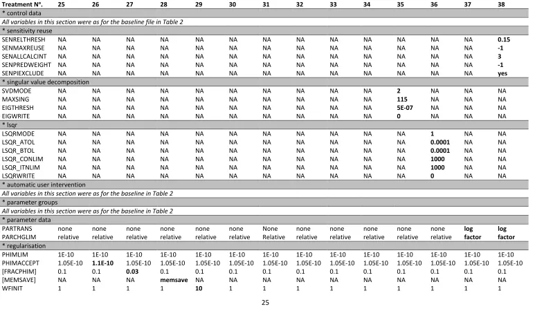
Table 3 Data from PEST control files used to conduct optimisation using Tikhonov regularisation. All optimisation runs were performed using ‘regularisation’ mode in PEST,
with 115 parameters, 56 parameter groups, 69 observation groups and 115 prior equations. Parameters shown in bold indicate variation from the baseline file. PEST control settings in the first column are described in the methods, and parameters in square brackets [] indicate optional use in the PEST control file. Each control file section is identified with an asterisk. NA = Not Applicable.
Treatment No. 25 26 27 28 29 30 31 32 33 34 35 36 37 38
* control data
All variables in this section were as for the baseline file in Table 2
* sensitivity reuse
SENRELTHRESH NA NA NA NA NA NA NA NA NA NA NA NA NA 0.15
SENMAXREUSE NA NA NA NA NA NA NA NA NA NA NA NA NA -1
SENALLCALCINT NA NA NA NA NA NA NA NA NA NA NA NA NA 3
SENPREDWEIGHT NA NA NA NA NA NA NA NA NA NA NA NA NA -1
SENPIEXCLUDE NA NA NA NA NA NA NA NA NA NA NA NA NA yes
* singular value decomposition
SVDMODE NA NA NA NA NA NA NA NA NA NA 2 NA NA NA
MAXSING NA NA NA NA NA NA NA NA NA NA 115 NA NA NA
EIGTHRESH NA NA NA NA NA NA NA NA NA NA 5E-07 NA NA NA
EIGWRITE NA NA NA NA NA NA NA NA NA NA 0 NA NA NA
* lsqr
LSQRMODE NA NA NA NA NA NA NA NA NA NA NA 1 NA NA
LSQR_ATOL NA NA NA NA NA NA NA NA NA NA NA 0.0001 NA NA
LSQR_BTOL NA NA NA NA NA NA NA NA NA NA NA 0.0001 NA NA
LSQR_CONLIM NA NA NA NA NA NA NA NA NA NA NA 1000 NA NA
LSQR_ITNLIM NA NA NA NA NA NA NA NA NA NA NA 1000 NA NA
LSQRWRITE NA NA NA NA NA NA NA NA NA NA NA 0 NA NA
* automatic user intervention
All variables in this section were as for the baseline in Table 2
* parameter groups
All variables in this section were as for the baseline in Table 2
* parameter data
PARTRANS none none none none none none None none none none none none log log
PARCHGLIM relative relative relative relative relative relative Relative relative relative relative relative relative factor factor
* regularisation
PHIMLIM 1E-10 1E-10 1E-10 1E-10 1E-10 1E-10 1E-10 1E-10 1E-10 1E-10 1E-10 1E-10 1E-10 1E-10
PHIMACCEPT 1.05E-10 1.1E-10 1.05E-10 1.05E-10 1.05E-10 1.05E-10 1.05E-10 1.05E-10 1.05E-10 1.05E-10 1.05E-10 1.05E-10 1.05E-10 1.05E-10
[FRACPHIM] 0.1 0.1 0.03 0.1 0.1 0.1 0.1 0.1 0.1 0.1 0.1 0.1 0.1 0.1
[MEMSAVE] NA NA NA memsave NA NA NA NA NA NA NA NA NA NA