Node centrality for continuous-time quantum walks

This is a repository copy of

Node centrality for continuous-time quantum walks

.

White Rose Research Online URL for this paper:

http://eprints.whiterose.ac.uk/85365/

Version: Accepted Version

Proceedings Paper:

Rossi, Luca, Torsello, Andrea and Hancock, Edwin R. orcid.org/0000-0003-4496-2028

(2014) Node centrality for continuous-time quantum walks. In: Structural, Syntactic, and

Statistical Pattern Recognition:Joint IAPR International Workshop, S+SSPR 2014,

Joensuu, Finland, August 20-22, 2014. Proceedings. Joint IAPR International Workshop

on Structural, Syntactic, and Statistical Pattern Recognition, S+SSPR 2014, 20-22 Aug

2014 Lecture Notes in Computer Science (including subseries Lecture Notes in Artificial

Intelligence and Lecture Notes in Bioinformatics) . Springer-Verlag , GBR , pp. 103-112.

https://doi.org/10.1007/978-3-662-44415-3_11

[email protected] https://eprints.whiterose.ac.uk/ Reuse

Items deposited in White Rose Research Online are protected by copyright, with all rights reserved unless indicated otherwise. They may be downloaded and/or printed for private study, or other acts as permitted by national copyright laws. The publisher or other rights holders may allow further reproduction and re-use of the full text version. This is indicated by the licence information on the White Rose Research Online record for the item.

Takedown

If you consider content in White Rose Research Online to be in breach of UK law, please notify us by

Node Centrality for

Continuous-Time Quantum Walks

Luca Rossi1_{, Andrea Torsello}2_{, and Edwin R. Hancock}3

1

School of Computer Science, University of Birmingham, UK

2

Department of Environmental Science, Informatics, and Statistics, Ca’ Foscari University of Venice, Italy

3

Department of Computer science, University of York, UK

Abstract. The study of complex networks has recently attracted

in-creasing interest because of the large variety of systems that can be modeled using graphs. A fundamental operation in the analysis of com-plex networks is that of measuring the centrality of a vertex. In this paper, we propose to measure vertex centrality using a continuous-time quantum walk. More specifically, we relate the importance of a vertex to the influence that its initial phase has on the interference patterns that emerge during the quantum walk evolution. To this end, we make use of the quantum Jensen-Shannon divergence between two suitably de-fined quantum states. We investigate how the importance varies as we change the initial state of the walk and the Hamiltonian of the system. We find that, for a suitable combination of the two, the importance of a vertex is almost linearly correlated with its degree. Finally, we evaluate the proposed measure on two commonly used networks.

Key words: Vertex Centrality, Complex Network, Quantum Walk,

Quan-tum Jensen-Shannon Divergence

1

Introduction

In recent years, an increasing number of researchers have turned their atten-tion to the study complex networks [1]. Complex network are ubiquitous in a large number of real-world systems. A non-exhaustive list of examples includes metabolic networks [2], protein interactions [3], brain networks [4] and scientific collaboration networks [5]. A fundamental task in complex network analysis is that of measuring the centrality of a vertex, i.e., its importance. To this end, a number of centrality indices have been introduced in the literature [1, 6–9]. Each of these captures different but equally significant aspects of vertex importance.

of the graph. More precisely, the closeness centrality is defined as the inverse of the sum of the distance of a vertex to the remaining nodes of the graph, i.e.,

CC(u) = _P n−1

n

v=1d(u,v) where d(u, v) denotes the shortest path distance between nodesuandv. The betweenness centrality [7] is a measure of the extent to which a given vertex lies on the paths between the remaining vertices, where the path may be either that of shortest length or a random walk between the nodes. If

sp(v1, v2) denotes the number of shortest paths from node v1 to node v2, and

sp(v1, u, v2) denotes the number of shortest paths fromv1tov2that pass through node u, the betweenness centrality of u is BC(u) = Pn

v1=1

Pn v2=1

sp(v1,u,v2)

sp(v1,v2) . Note that this definition assumes that the communication takes place along the shortest path between two vertices. A number of measures have been introduced to account for alternative scenarios in which the information is allowed to flow through different paths [1, 6–8].

Recently, there has also been a surge of interest in using quantum walks as a primitive for designing novel quantum algorithms on graph structures [11]. Quan-tum walks on graphs represent the quanQuan-tum mechanical analogue of the classical random walk on a graph. Despite being similar in their definition, the dynamics of the two walks can be remarkably different. In the classical case the evolution of the walk is governed by a double stochastic matrix, while in the quantum case the evolution is governed by a unitary matrix, thus rendering the walk re-versible and non-ergodic. Moreover, the state vector of the classical random walk is real-valued, while in the quantum case the state vector is complex-valued. As there is no constraint on the sign and phase of the amplitudes, different paths are allowed to interfere with each other in both constructive and destructive ways. This in turn gives rise to faster hitting times and reduces the problems of tottering observed in classical random walks [11].

In this paper, we propose to measure the centrality of a vertex using a continuous-time quantum walk. More specifically, we relate the importance of a vertex to the influence that its initial phase has on the evolution of a suitably de-fined quantum walk. To this end, we make use of the quantum Jensen-Shannon divergence, a recently introduced generalisation of the classical Jensen-Shannon divergence to quantum states [12]. Just as the classical Jensen-Shannon diver-gence [13], the quantum Jensen-Shannon diverdiver-gence is symmetric, bounded and always defined. From a physical perspective, the QJSD is computed from density matrices, whose entries are observables. As a consequence, it should be possible, at least in theory, to design a quantum algorithm to compute the QJSD cen-trality that could benefit from the power of quantum computers. However, the design of such an algorithm is beyond the scope of this paper.

Node Centrality for Continuous-Time Quantum Walks 3

2

Quantum Mechanical Background

The continuous-time quantum walk [14] is a natural quantum analogue of the classical random walk. Given a graphG= (V, E), classical random walks model a diffusion process over the node set V, and have proven to be a useful tool in the analysis of its structure. Similarly, the continuous-time quantum walk is defined as a dynamical process over the vertices of the graph. By contrast to the classical case, where the state vector is constrained to lie in a probability space, in the quantum case the state of the system is defined through a vector of complex amplitudes over the node setV whose squared norm sums to unity over the nodes of the graph, with no restriction on their sign or complex phase. These phase differences allow interference effects to take place. Moreover, in the quantum case the evolution of the state vector of the walker is governed by a complex valued unitary matrix, whereas the dynamics of the classical random walk is governed by a stochastic matrix. Hence the evolution of the quantum walk is reversible, implying that quantum walks are non-ergodic and do not possess a limiting distribution. As a result, the behaviour of classical and quantum walks differs significantly, and quantum walks possess a number of interesting properties not exhibited by classical random walks.

More formally, using the Dirac notation, we denote the basis state corre-sponding to the walk being at vertexu∈V as|ui. A general state of the walk is a complex linear combination of the basis states, such that the state of the walk at timet is defined as

|ψti=

X

u∈V

αu(t)|ui (1)

where the amplitudeαu(t)∈Cand|ψti ∈C|V| are both complex.

At each instant in time the probability of the walker being at a particular vertex of the graph is given by the square of the norm of the amplitude of the relative state. Let Xt _{be a random variable giving the location of the walker}

at time t. Then the probability of the walker being at the vertex u at timet

is given by Pr(Xt_{=u) =α}

u(t)α∗u(t), where α∗u(t) is the complex conjugate of αu(t). Moreover Pu∈V αu(t)α∗u(t) = 1 and αu(t)α∗u(t) ∈ [0,1], for all u ∈ V, t∈R+_.

The evolution of the walk is then given by the Schr¨odinger equation, where we take the time-independent Hamiltonian of the system to be the graph Laplacian, yielding

∂

∂t|ψti=−iL|ψti. (2)

Given an initial state|ψ0i, we can solve Eq. (2) to determine the state vector at timet

|ψti=e−iLt|ψ0i. (3)

Finally, we can compute the spectral decomposition of the graph Laplacian

L = ΦΛΦ⊤_{, where Φ is the n×n matrix Φ = (φ}

1|φ2|...|φj|...|φn) with the

ordered eigenvectors φjs of L as columns andΛ = diag(λ1, λ2, ..., λj, ..., λn) is

then×ndiagonal matrix with the ordered eigenvaluesλjofLas elements, such

that 0 = λ1 ≤ λ2 ≤ ... ≤ λn. Using the spectral decomposition of the graph

Laplacian and the fact that exp[−iLt] =Φexp[−iΛt]Φ⊤ _{we can then write}

|ψti=Φe−iΛtΦ⊤|ψ0i. (4)

2.1 Quantum Jensen-Shannon Divergence

Thedensity operator(ordensity matrix) is introduced in quantum mechanics to describe a system whose state is an ensemble of pure quantum states|ψii, each

with probability pi. The density operator of such a system is defined as

ρ=X

i

pi|ψii hψi|. (5)

The von Neumann entropy [15]HN of a density operatorρis defined as

HN =−tr(ρlogρ) =− X

i

ξilnξi (6)

where ξ1, . . . , ξn are the eigenvalues of ρ. If hψi|ρ|ψii = 1, i.e., the quantum

system is a pure state |ψii with probability pi = 1, then the Von Neumann

entropyHN(ρ) =−tr(ρlogρ) is zero. On other hand, for a mixed state described

by the density operatorσwe have a non zero Von Neumann entropy associated with it.

With the Von Neumann entropy to hand, the quantum Jensen-Shannon di-vergence between two density operatorsρandσis defined as

DJ S(ρ, σ) =HN ρ+σ

2

−1

2HN(ρ)− 1

2HN(σ) (7)

This quantity is always well defined, symmetric and positive definite. Finally, it can also be shown that DJ S(ρ, σ) is bounded, i.e., 0≤DJ S(ρ, σ)≤1.

3

QJSD Centrality

In order to measure the centrality of vertex v, we define two quantum walks where v is initially set to be in phase and in antiphase with the respect to the remaining nodes. Let the normalised graph Laplacian be the Hamiltonian of our system, and let

ψv₀−

=P

u∈V αvu−(0)|uiand ψv₀+

=P

u∈V αvu+(0)|uidenote

the quantum walks onGwith initial amplitudes

αv_j−(0) =

(

−

√

dj

C ifj=v

+ √

dj

C otherwise

αv_j+(0) =n+ √

dj

Node Centrality for Continuous-Time Quantum Walks 5

whereCis the normalisation constant such that probabilities sum to 1. In other words, we define the initial amplitude to be proportional to the square root of the node degrees. Finally, let ρv+ andρ_v− be the density operators which describe

the ensembles of quantum states ψv_t−

and ψv_t+

respectively, i.e.,

ρv− = lim

T→∞ 1

T Z T

0

ψ_tv− ψv_t−

dt ρ_v+ = lim

T→∞ 1

T Z T

0

ψ_tv+ ψv_t+

dt (9)

Given this setting, we can measure how the initial phase of the vertex v

affects the evolution of the quantum walks by computing the distance between the quantum states defined by ρv− and ρv+. That is, we define the quantum

Jensen-Shannon divergence (QJSD) centrality of a vertexv as

CQJ SD(v) =DJ S(ρv−, ρ_v+) (10)

Note that the computational complexity of the QJSD centrality is bounded by that of computing the eigendecomposition of the graph laplacian, i.e.,O(n3_). LetΦΛΦ⊤_{be the spectral decomposition of the graph normalised Laplacian and} let Pλ = Pµk=1(λ)φλ,kφ⊤λ,k be the projection operator on the subspace spanned

by the µ(λ) eigenvectors φλ,k associated with the eigenvalue λ of the graph

normalised Laplacian. Rossi et al. [16] have shown that ρ_∞ = Pm

λ=1Pλρ0Pλ⊤,

where m denotes the number of unique eigenvalues of the graph normalised Laplacian. Note that as a consequence of Eq. ??we have thatρv− and ρv+ are

simultaneously diagonalisable. That is, there exist a single invertible matrix M

such thatM−1_ρ

v−M andM− 1_ρ

v+M are diagonal. More precisely, hereM =Φ, the n×n matrix Φ= (φ1|φ2|...|φj|...|φn) with the ordered eigenvectors φjs of

the Hamiltonian as columns.

3.1 Relation with Degree Centrality

We are now interested in studying the relation between the QJSD centrality and the degree centrality. It has been shown, for example, that the degree and the betweenness centrality are highly correlated [17]. This should not come as a surprise, as we expect high degree vertices to be more often included in the shortest path along a pairs of vertices.

Let the initial states of the walks be defined as in Eq. 8 and let the normalised Laplacian be the Hamiltonian of our system. We start by observing that

ψ₀v+

=

P

u∈V αuv+(0)|ui corresponds to the eigenvector φ0 associated with the zero eigenvalue of the Hamiltonian, and as a consequence

ψ₀v+

will remain constant over time. In other words, we have that ρv+ =

ψv₀+ ψv₀+

. Note that the

spectrum ofρv+ is composed of a single eigenvectorφ₀with eigenvalue equal to 1. Moreover, recall from Eq.??thatρv− andρ_v+ are co-diagonalisable matrices.

As a result, each eigenvalue ofρv−+ρv+is a sum of eigenvalues ofρv− andρv+.

More precisely, when the two walks are initialised as in Eq. 8, all the eigenvalues

µi of

ρ_v−+ρv+

2 will be equal to the eigenvalues ofρv−, except for the eigenvalue

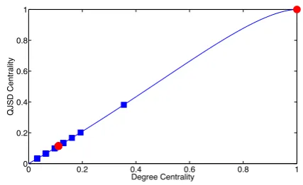
0 0.2 0.4 0.6 0.8 1 0 0.2 0.4 0.6 0.8 1 Degree Centrality Q JSD C e n tra lit y

Fig. 1.The correlation between degree and QJSD centrality, for a star graph (red dots)

and a scale-free graph (blue squares). The blue line shows the predicted dependency between the two centrality indices.

We now show that, as a consequence of this, the QJSD centrality is pro-portional to the degree centrality. Note that since ρv+ has a single non-zero eigenvalue which is equal to 1, we have that HN(ρv+) = 0. As a consequence of this and of Eq. 7, we have that

DJ S(ρv−, ρv+) =HN

ρv−+ρv+

2

−1₂HN(ρv−)

=−µ0₂+ 1log2

µ0+ 1

2 −

X

i6=0

µi

2 log2

µi 2 + 1 2 X i

µilog2µi

=µ0+ 1

2 −

µ0+ 1

2 log2(µ0+ 1) +

X

i6=0

µi

2 − 1 2

X

i6=0

µilog2µi+

1 2

X

i

µilog2µi

= 1−1

2log2(µ0+ 1) +

µ0 2 log2

µ0

µ0+ 1

(11)

whereµidenotes theith eigenvalue ofρv− and we used the fact that

P

iµi= 1.

We now proceed to show that µ0 is proportional to the degree of node v, and therefore the QJSD centrality is proportional to the degree centrality. In fact, we have that

µ0=hφ0|ρ0|φ0i=φ0

ψ₀v−

2

=

1− dv

|E|

2

(12)

wheredv is the degree of vand|E| denotes the number of edges in the graph.

Node Centrality for Continuous-Time Quantum Walks 7

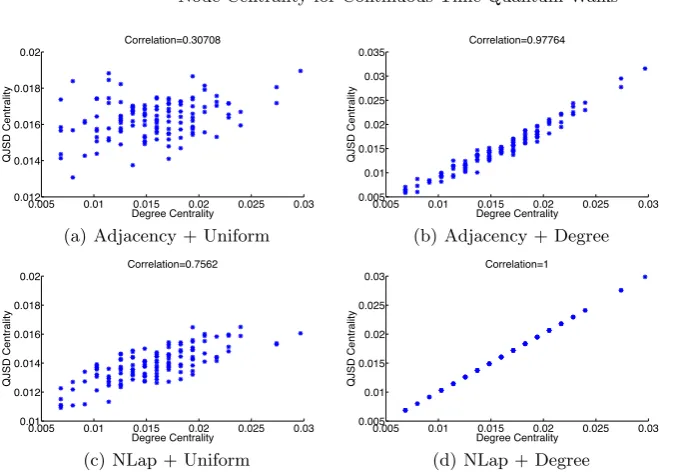
0.005 0.01 0.015 0.02 0.025 0.03

0.012 0.014 0.016 0.018 0.02 Correlation=0.30708 Degree Centrality Q JSD C e n tra lit y

(a) Adjacency + Uniform

0.005 0.01 0.015 0.02 0.025 0.03 0.005 0.01 0.015 0.02 0.025 0.03 0.035 Correlation=0.97764 Degree Centrality Q JSD C e n tra lit y

(b) Adjacency + Degree

0.005 0.01 0.015 0.02 0.025 0.03

0.01 0.012 0.014 0.016 0.018 0.02 Correlation=0.7562 Degree Centrality Q JSD C e n tra lit y

(c) NLap + Uniform

0.005 0.01 0.015 0.02 0.025 0.03 0.005 0.01 0.015 0.02 0.025 0.03 Correlation=1 Degree Centrality Q JSD C e n tra lit y

(d) NLap + Degree

Fig. 2.Correlation between the QJSD centrality and the degree centrality for different

choices of the Hamiltonian (adjacency matrix or normalised Laplacian) and of the initial state (normalised uniform distribution or normalised degree distribution).

edge set. Note that the non-linearity of the correlation becomes evident only for those nodes with degree close to|E|, for which we have that dv

|E| ≈0 and thus

µ0≈1 +_|d_Ev_| 2

.

So far we assumed that the Hamiltonian of the quantum walk is the graph normalised Laplacian. However, any Hermitian operator encoding the structure of the graph can be chosen as an alternative. Similarly, there is no constraint on the initial state of the walk, as long as it is a valid amplitude vector. Fig. 2 shows the correlation between the QJSD centrality and the degree centrality computed on a stochastic Kronecker graph for different choices of the initial state and the Hamiltonian. More specifically, we let the Hamiltonian be either the adjacency matrix or the normalised Laplacian of the graph, while the initial state is either proportional to the node degree as in Eq. 8 or uniformly equal to 1/√n, wheren

denotes the number of nodes in the graph. As expected, our centrality measure is strongly correlated with the degree centrality when the Hamiltonian is the graph normalised Laplacian and the initial state is proportional to the node degree (see Fig. 2(d)). In general, we see that when the starting state is proportional to the node degree, the correlation tends to be very high, while the choice of a uniform initial state leads to a value of the centrality which is less dependent on the node degree.

1

2

3

4

Fig. 3.Zachary’s karate club network, where we have drawn each node with a diameter

that is proportional to its QJSD centrality.

walk start from a uniform amplitude vector and choosing the adjacency matrix as the Hamiltonian. Moreover, in order to balance the strength of the positive and negative signals, i.e., the contribution of the node amplitudes with either positive or negative phases, we let the magnitude of the initial amplitude on the node being analysed be equal to the sum of the amplitudes on the remaining nodes, which gives the initial state

αv−

j (0) = (

−_√1

2 ifj =v +√ 1

2(|V|−1) otherwise

αv+

j (0) = (

+_√1

2 ifj=v +√ 1

2(|V|−1) otherwise

.

(13)

4

Experimental Evaluation

Node Centrality for Continuous-Time Quantum Walks 9

ACCIAIUOL

ALBIZZI BARBADORI

BISCHERI CASTELLAN

GINORI

GUADAGNI

LAMBERTES MEDICI

PAZZI

PERUZZI

RIDOLFI

SALVIATI

STROZZI

TORNABUON

Fig. 4.Padgett’s network of marriages between eminent Florentine families in the 15th

century [19]. We omit the Pucci, which had no marriage ties with other families.

Family Centrality Family Centrality Family Centrality

Medici 0.4867 Castellan 0.3245 Salviati 0.2248 Ridolfi 0.4619 Barbadori 0.3205 Ginori 0.1993 Strozzi 0.4192 Albizzi 0.3172 Acciaiuol 0.1534 Tornabuon 0.4041 Guadagni 0.3091 Lambertes 0.1267 Bischeri 0.3586 Peruzzi 0.2990 Pazzi 0.1126

Table 1.The QJSD centrality of the families of Padgett’s network [19].

Padgett’s network of marriages is depicted in Fig. 4. In Table 1, we show the ranking of the 15 families according to their QJSD centrality. As expected, the Medici easily outperform the Strozzi , who are their main rivals. This agrees with the historical view that Medici’s supremacy was largely due to their skills in manipulating the marriage network. Interestingly the Pazzi, which is the most loosely connected family of the graph, achieve the lowest centrality. Note also that the Ridolfi family, which connect two of the most influential families at that time, the Medici and the Strozzi, is assigned a high centrality. Moreover, the Tornabuon, which form a tightly connected clique together with the Medici and the Ridolfi, is the fourth most central node of the network.

5

Conclusions

Thus, we have proposed an alternative starting state where the contribution of the node amplitudes with positive and negative phases is equal. Finally, we have evaluated the resulting measure to two commonly used network models.

Acknowledgments. Edwin Hancock was supported by a Royal Society Wolfson Research Merit Award.

References

1. Estrada, E.: The Structure of Complex Networks. Oxford University Press (2011) 2. Jeong, H., Tombor, B., Albert, R., Oltvai, Z., Barab´asi, A.: The large-scale

orga-nization of metabolic networks. Nature407(2000) 651–654

3. Ito, T., Chiba, T., Ozawa, R., Yoshida, M., Hattori, M., Sakaki, Y.: A comprehen-sive two-hybrid analysis to explore the yeast protein interactome. Proceedings of the National Academy of Sciences98(2001) 4569

4. Sporns, O.: Network analysis, complexity, and brain function. Complexity8(2002) 56–60

5. Newman, M.: Scientific collaboration networks. i. network construction and fun-damental results. Physical review E64(2001) 016131

6. Freeman, L.C.: A set of measures of centrality based on betweenness. Sociometry (1977) 35–41

7. Freeman, L.C.: Centrality in social networks conceptual clarification. Social net-works1(1979) 215–239

8. Newman, M.E.: A measure of betweenness centrality based on random walks. Social networks27(2005) 39–54

9. Bonacich, P.: Power and centrality: A family of measures. American journal of sociology (1987) 1170–1182

10. Stanley, W., Faust, K.: Social network analysis: methods and applications. Cam-bridge: Cambridge University (1994)

11. Kempe, J.: Quantum random walks: an introductory overview. Contemporary Physics44(2003) 307–327

12. Lamberti, P., Majtey, A., Borras, A., Casas, M., Plastino, A.: Metric character of the quantum jensen-shannon divergence. Physical Review A77(2008) 052311 13. Lin, J.: Divergence measures based on the shannon entropy. Information Theory,

IEEE Transactions on37(1991) 145–151

14. Farhi, E., Gutmann, S.: Quantum computation and decision trees. Physical Review A58(1998) 915

15. Nielsen, M.A., Chuang, I.L.: Quantum computation and quantum information. Cambridge university press (2010)

16. Rossi, L., Torsello, A., Hancock, E.R., Wilson, R.C.: Characterizing graph symme-tries through quantum jensen-shannon divergence. Physical Review E88(2013) 032806

17. Lee, C.Y.: Correlations among centrality measures in complex networks. arXiv preprint physics/0605220 (2006)

18. Zachary, W.: An information flow modelfor conflict and fission in small groups1. Journal of anthropological research33(1977) 452–473