White Rose Research Online URL for this paper:
http://eprints.whiterose.ac.uk/85654/
Version: Accepted Version
Article:
Jones, B., Kerrigan, E.C., Morrison, J.F. et al. (1 more author) (2011) Flow estimation of
boundary layers using DNS-based wall shear information. International Journal of Control,
84 (8). pp. 1310-1325. ISSN 0020-7179
https://doi.org/10.1080/00207179.2011.593000
[email protected] https://eprints.whiterose.ac.uk/ Reuse
Unless indicated otherwise, fulltext items are protected by copyright with all rights reserved. The copyright exception in section 29 of the Copyright, Designs and Patents Act 1988 allows the making of a single copy solely for the purpose of non-commercial research or private study within the limits of fair dealing. The publisher or other rights-holder may allow further reproduction and re-use of this version - refer to the White Rose Research Online record for this item. Where records identify the publisher as the copyright holder, users can verify any specific terms of use on the publisher’s website.
Takedown
If you consider content in White Rose Research Online to be in breach of UK law, please notify us by
International Journal of Control Vol. 00, No. 00, Month 200x, 1–22
RESEARCH ARTICLE
Flow Estimation of Boundary Layers Using DNS Based Wall Shear Information
Bryn Ll. Jonesa∗, Eric C. Kerriganb,c, Jonathan F. Morrisoncand Tamer A. Zakid
aThe Department of Automatic Control and Systems Engineering, University of Sheffield, UK;bDepartment of
Electrical and Electronic Engineering, Imperial College London, UK;cDepartment of Aeronautics, Imperial
College London, UK;dDepartment of Mechanical Engineering, Imperial College London, UK.
(Received 00 Month 200x; final version received 00 Month 200x)
This paper investigates the problem of obtaining a state-space model of the disturbance evolution that precedes turbulent flow across aerodynamic surfaces. This problem is challenging since the flow is governed by nonlinear, partial differential-algebraic equations for which there currently exists no efficient controller/estimator synthesis techniques. A sequence of model approx-imations is employed to yield a linear, low-order state-space model, to which standard tools of control theory can be applied. One of the novelties of this paper is the application of an algorithm that converts a system of differential-algebraic equations into one of ordinary differential equations. This enables straightforward satisfaction of boundary conditions whilst dispensing with the need for parallel flow approximations and velocity-vorticity transformations. The efficacy of the model is demonstrated by the synthesis of a Kalman filter that clearly reconstructs the characteristic features of the flow, using only wall velocity gradient information obtained from a high-fidelity nonlinear simulation.
Keywords:Turbulence, nonlinear equations, partial differential equations, descriptor systems, model approximation, boundary conditions.
1 Introduction
In a recent research agenda, the Advisory Council for Aeronautics Research in Europe (ACARE) rec-ommended a 50% reduction in fuel consumption (per passenger kilometre) of all new aircraft by the year 2020 (Arg¨uelles et al. 2001), for obvious economic and environmental reasons. However, it is widely accepted that this target is unlikely to be met unless novel flow control technologies emerge, which are capable of manipulating the surrounding airflow to reduce the drag force exerted on an air-craft (Gad-el-Hak 2000). In practice, it is likely that the sensors and actuators of such a scheme (Arthur et al. 2006) will be located on the aircraft surfaces, thus necessitating the use of an observer to estimate flow parameters away from the wall. Knowledge of these estimates may subsequently enable improved actuation towards a more desirable flow-field.
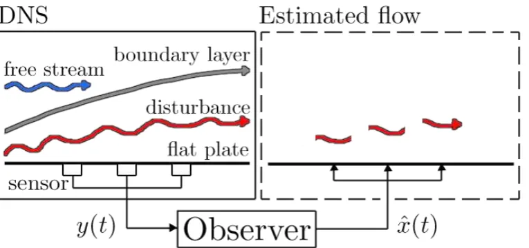
In order to synthesise an observer, a model of the system is required. In the present work the system is taken to be a boundary layer (Schlichting and Gersten 2000, White 2003) evolving over a flat plate, as depicted in Figure 1. The term ‘boundary layer’ simply refers to the layer of fluid next to a bounding surface. Here, the bounding surface is a flat plate, which can be considered a simplified aircraft wing. At subsonic velocities this type of flow is governed by the incompressible Navier-Stokes equations:
ρ∂~v
∂t =µ∆~v−ρ~v·∇~v−∇p+
~f, (1a)
0=∇·~v, (1b)
This work was supported by the EPSRC.
∗Corresponding author. Email: [email protected]
ISSN: 0020-7179 print/ISSN 1366-5820 online c
with initial and boundary conditions:
~v(ζ,0) =~v0(ζ) ∀ζ ∈Ω, (1c)
~v(ζ,t) =~g(ζ,t) ∀(ζ,t)∈∂Ω×[0,tf], (1d)
where the velocity of the fluid is~v:Ω×R+ 7→R3,p:Ω×R+ 7→Ris the pressure,~f :Ω×R+7→R3 is a vector of external forces,~g:∂Ω×R+ 7→R3 is a vector of boundary conditions, and~v
0∈R3 is a vector of initial velocities. The density and viscosity of the fluid (here assumed constant) areρ,µ∈R+, respectively, andtf ∈R+ is the endpoint of the time interval. The gradient operator is denoted by ∇
whilst∆ and∇·denote the Laplace and divergence operators, respectively. The flow evolves within a domain Ω⊂R3 with three spatial dimensions and a boundary∂Ω, and ζ ∈Ω is a point within the domain. Throughout this paper sans serif fonts will represent parameters used to describe the flow system, whilst serif fonts will denote (discretised) vectors and matrices.
The Navier-Stokes equations (1) are a coupled system of nonlinear, partial differential-algebraic equa-tions, for which no general controller/estimator synthesis techniques currently exist. In order to simplify analysis, the majority of researchers have focussed their efforts upon relatively well understood flows. A particular case that has received much attention is that of channel flow, e.g. Hoepffner et al. (2005), Hogberg et al. (2003), Baramov et al. (2004), McKernan et al. (2007), Chughtai and Werner (2010), where the mean (time-averaged) flow is parallel to the walls and fully developed in the sense that it is invariant in the streamwise direction. A convenient consequence of this fact is that it enables a relatively straightforward analytic reformulation of (1) into an equivalent system expressed in terms of so-called ‘divergence-free’ variables of wall-normal velocity and vorticity. These variables implicitly satisfy the incompressibility constraint (1b) thus allowing the flow dynamics, after spatial discretisation, to be de-scribed by ordinary differential equations (ODEs), rather than differential-algebraic equations (DAEs). Hence, the flow can be modelled as a conventional state-space system, rather than a descriptor (or im-plicit) state-space system for which far fewer established control-theoretic tools exist.
In contrast, the mean flow of a boundary layer is non-parallel since it varies with distance travelled in the streamwise direction. In an effort to recast the system in terms of a divergence-free basis, a parallel flow assumption is commonly employed, e.g. Hoepffner and Brandt (2008). In the present work the need for this assumption is avoided by employing a more flexible modelling technique that produces a state-space model without the need for an analytical reformulation of the governing equations. To complete the state-space model, a disturbance model is included as well as Direct Numerical Simulation (DNS) based measurements of the streamwise and spanwise wall shear (wall-normal velocity gradient) at three evenly spaced locations along the plate. Based on this model, a time-varying Kalman filter is synthesised that produces estimates of the in-plane velocity fields. The overall scheme is sketched in Figure 1.
Two-dimensional control of boundary layers has been considered (Baker et al. 2002), as has Tollmien-Schlichting wave cancellation (Sturzebecher and Nitsche 2003), but to the best of the authors’ knowl-edge, this is the first work to attempt flow estimation of a three-dimensional, non-parallel and unsteady boundary layer by employing an estimator derived from a physically based model and using practically implementable sensors mounted in the bounding surface. For the special case where disturbances are time-independent, one can view perturbation growth within a (non-parallel) boundary layer as a process that evolves in space, rather than in time, and control of such a system has been considered (Cathalifaud and Bewley 2004). However, in practical control terms, the temporal dynamics of sensors and actua-tors will likely form an important part of any model used for controller/estimator synthesis, and so in this paper, the growth of boundary layer disturbances is viewed as a process that evolves in time (i.e. is unsteady), within a fixed volume of space.
The sequence of modelling steps described in this paper, namely linearisation, spatial discretisation and the numerical conversion of DAEs into ODEs, are very general in nature and thus can be applied to a wide range of fluid flow systems to obtain simple control models.
Figure 1. Sketch of the estimation problem. The observer constructs estimates ˆx(t)of the true velocity perturbation (shown in red) above the sensors, using only measurementsy(t)of the streamwise and spanwise wall shears. Note that in realistic flows, the boundary layer interface is not as smooth and well defined as sketched here.
necessarily spawned a large body of complex terminology and phraseology that can be discouraging to control practitioners interested in controlling fluid flows. Therefore, the current exposition aims to employ and define only those fluid mechanics concepts most relevant to obtaining a model for control or estimation. At the same time, and for the benefit of a fluid mechanics audience, every effort has been made to ensure the references are as complete and the paper as self-contained as possible.
This paper is organised as follows. Section 2 describes the boundary layer DNS database and the underlying physical model. Section 3 discusses the validity of a linear approximation to the boundary layer equations. In Section 4 the linearised system is spatially discretised to yield a finite-dimensional descriptor state-space model, together with a technique for easily enforcing boundary conditions. Sec-tion 5 describes a method for converting this descriptor state-space system into a standard state-space system, which, in Section 6 is augmented with a disturbance model and wall shear measurements. Based on the resulting model, a time-varying Kalman filter is synthesised and the velocity field estimates are presented in Section 7, with conclusions in Section 8.
As a final note in this section, it is stressed that the control and estimation of fluid flows poses chal-lenging research questions, many of which are not tackled in this paper. For example, this paper does not address the issue of optimal location of sensors and actuators. Nor does it address the issue of guaranteeing that controllers and estimators based on approximate models of finite state dimension will actually perform well on the underlying infinite-dimensional plant. These issues are addressed, for exam-ple, in Naguib et al. (2010), Bagheri et al. (2009), Reinschke and Smith (2003) and Jones and Kerrigan (2010).
2 Description of the DNS Database
[image:4.595.100.483.46.226.2]Figure 2. Sketch of the computational domain and coordinate system. Figure from Naguib et al. (2010).
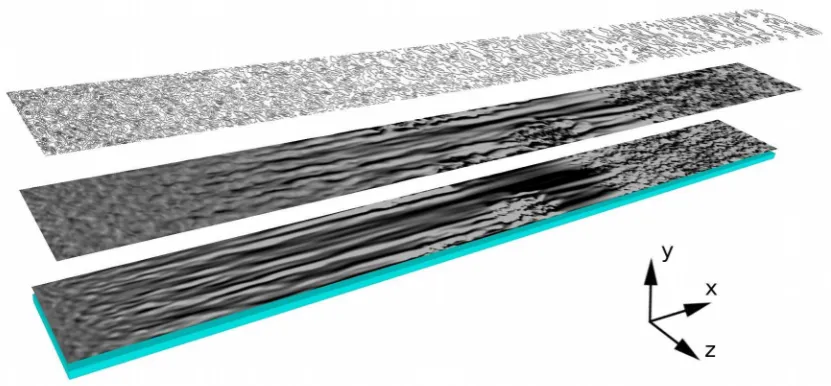
Figure 3. DNS snapshot. The flow is from left to right. Shaded regions represent streamwise velocity perturbations at three different heights above the wall. The lower two planes are within the boundary layer whilst the upper plane is in the free-stream.
particle to travel a total distance of 2400δ0at the free-stream velocityU∞. A snapshot of the DNS data is shown in Figure 3 and depicts three planes parallel to the wall. The lower planes are inside the bound-ary layer whilst the uppermost is in the free-stream. The contours depict velocity perturbations in the streamwise direction. The flow is initially laminar and characterised by long streamwise perturbations, or ‘streaks’, that are initiated by disturbances in the free-stream penetrating the boundary layer (Zaki and Saha 2009). The streaks grow in magnitude and develop secondary instabilities (Vaughan and Zaki 2011) that lead to localised breakdown into turbulent spots, with the spots merging to form a fully-turbulent boundary layer. Transition to turbulence via this mechanism is known as ‘bypass’ transition since, for moderate sizes of disturbances, the Tollmien-Schlichting (‘modal’) wave development (Sturzebecher and Nitsche 2003) is bypassed. This process can lead to the transient growth phenomenon, explained in the next section, as opposed to the exponential growth of Tollmien-Schlichting waves.
[image:5.595.80.496.264.457.2]3 Transient Growth and Linearisation
Transition to turbulence has traditionally been investigated by linearising the flow system around an equilibrium and inspecting the eigenvalues of the linearised system. However, the predictions of this hydrodynamic stability theory are well known to contradict physical experiments (Butler and Farrell 1992), with the latter often displaying instability (turbulence) despite the eigenvalues of the linearised system residing in the complex left-half-plane. In recent years, a reconciliation of these findings has been provided by non-modal stability theory, e.g. Butler and Farrell (1992), Trefethen et al. (1993), Schmid (2007), whereby the eigenfunction alignment of the linearised flow system is analysed. These eigen-functions are known to by highly nonorthogonal. Consequently, small, three-dimensional perturbations to the mean flow can be amplified by several orders of magnitude via a linear mechanism, despite all the eigenvalues being stable. This transient growth, if large enough, can initiate so-called ‘bypass’ transition to turbulence.
A linear, transient growth model of the current boundary layer is obtained as follows. The Navier-Stokes equations (1) are first made nondimensional by scaling all parameters by the inlet boundary layer thicknessδ0and the free-stream velocityU∞. Subsequent linearisation about a nominal mean flow yields the following set of perturbation equations (Aamo and Krstic 2003, p. 16):
∂u
∂t =−u
∂U
∂x−U
∂u
∂x−v
∂U
∂y −V
∂u
∂y−w
∂U
∂z −W
∂u
∂z−
∂p
∂x+
1
R
∂2u ∂x2 +
∂2u ∂y2+
∂2u ∂z2
,
∂v
∂t =−u
∂V
∂x −U
∂v
∂x−v
∂V
∂y −V
∂v
∂y−w
∂V
∂z −W
∂v
∂z−
∂p
∂y+
1
R
∂2v ∂x2+
∂2v ∂y2+
∂2v ∂z2
,
∂w
∂t =−u
∂W
∂x −U
∂w
∂x−v
∂W
∂y −V
∂w
∂y−w
∂W
∂z −W
∂w
∂z −
∂p
∂z+
1
R
∂2w
∂x2 + ∂2w
∂y2 + ∂2w
∂z2
,
0=∂u
∂x+
∂v
∂y+
∂w
∂z, (2)
whereR:=U∞δ0/νis the Reynolds number,ν:=µ/ρis the kinematic viscosity of the fluid,U,VandW are the average streamwise, wall-normal and spanwise velocities, respectively, whilstu,v,wandpare the corresponding perturbation velocities and pressure. For clarity, the spatial and temporal dependence of each of the variables is not shown here, but it should be noted thatu,v,wandpare each real-valued functions ofx,y,zandt, whereas the mean-flow velocities are real valued functions ofx,yandz, only. Since the system of interest is the transient growth region of a laminar, flat-plate boundary layer subject to zero streamwise pressure gradient, the following simplifying assumptions can be employed:
• Two-dimensional mean flow, i.e.W, ∂∂Uz, ∂∂Vz, ∂∂Wz =0. • Negligible streamwise pressure gradient, i.e. ∂∂px ≈0.
• Negligible second-order streamwise velocity gradients, i.e. ∂∂2xu2, ∂2v ∂x2,
∂2w ∂x2 ≈0.
system(2)reduces to: ∂u
∂t =−u
∂U
∂x −U
∂u
∂x−v
∂U
∂y −V
∂u
∂y+
1
R
∂2u ∂y2 +
∂2u ∂z2
,
∂v
∂t =−u
∂V
∂x −U
∂v
∂x−v
∂V
∂y −V
∂v
∂y−
∂p
∂y+
1
R
∂2v ∂y2+
∂2v ∂z2
,
∂w
∂t =−U
∂w
∂x −V
∂w
∂y−
∂p
∂z+
1
R
∂2w
∂y2 + ∂2w
∂z2
,
0=∂u
∂x+
∂v
∂y+
∂w
∂z. (3)
where the mean-flow velocitiesU,Vare now functions ofx,yonly. The interested reader may wish to compare (3) with the linearised equations obtained for channel flow (Aamo and Krstic 2003, p 21). For boundary conditions of (3), the following are assumed (Andersson et al. 1999):
u(x,0,z,t) =0, v(x,0,z,t) =0, w(x,0,z,t) =0,
u(x,ymax,z,t) =0, p(x,ymax,z,t) =0, w(x,ymax,z,t) =0, (4a)
where ymax →∞, although in practice this is set to a large but finite value. In a realistic estimation
problem, the initial condition of the flow will be unknown, in which case it is assumed to be zero:
u(x,y,z,0), v(x,y,z,0),w(x,y,z,0), p(x,y,z,0) =0. (4b)
The equations in (3) are known as the Linearised Boundary Region Equations (LBRE) (Leib et al. 1999), and have been shown to accurately predict the evolution of streaky boundary layer disturbances in re-sponse to external forcing.
The mean flow quantitiesUandVin (3) are computed by solving the Blasius equation forF(η)and its derivatives:
2F′′′(η) +F(η)F′′(η) =0, (5a)
whereη:=y(νx/U∞)−1/2,F′(η):=dFdη(η) and (5a) has the boundary conditions:
F(0) =F′(0) =0, F′(η)→1 as η→∞. (5b)
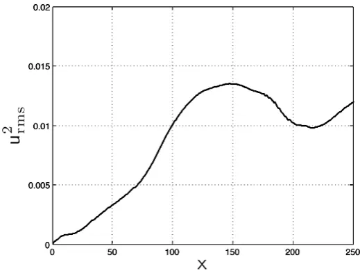
Figure 4. Mean-square streamwise velocity perturbations versusx, fory=0.69. Linear growth occurs in the region 20/x/60. Recall thatx(0)corresponds to the origin of the axes in Figure 2.
follows:
U(x,y) =F′(η),
V(x,y) =1
2 r
ν
U∞x
ηF′(η)−F(η),
∂U(x,y)
∂x =−
η 2xF
′′(η),
∂V(x,y)
∂x =−
1 4x32
r ν
U∞
η2F′′(η) +ηF′(η)−F(η),
∂U(x,y)
∂y =
r
U∞ νxF
′′(η),
∂V(x,y)
∂y =
η 2xF
′′(η). (5c)
The streamwise region of validity for the linear model can be deduced from the DNS data by studying the downstream evolution of the kinetic energy of theuperturbations. Figure 4 shows the streamwise evolution of the mean-squareuperturbations at a height above the wall ofy=0.69, corresponding to the wall-normal location of maximum disturbance energy. Linear (algebraic) growth appears for 20/x/
60 (Naguib et al. 2010).
4 Spatial Discretisation
[image:8.595.153.413.48.243.2]4.1 Spanwise discretisation
Referring to Figure 3, since the flow is periodic in the spanwise direction, the Fourier transform can be employed as follows:
u(x,y,z,t)≈R Nz−1
∑
nz=0
˜
u(x,y,t)eiβz
!
, (6)
wherei:=√−1,nzis the harmonic number, β :=2πnz/Lzis a wavenumber,Lz is the wavelength in the spanwise direction andNz is finite and represents the truncation of the series. Similar expressions are obtained for the remaining perturbation variables. Substituting these into (3), yields the following systemfor each wavenumberβ:
∂u˜ ∂t =−u˜
∂U
∂x−U
∂u˜ ∂x−v˜
∂U
∂y −V
∂u˜ ∂y+
1
R
∂2u˜ ∂y2−β
2u˜
,
∂v˜ ∂t =−u˜
∂V
∂x −U
∂v˜ ∂x−v˜
∂V
∂y −V
∂v˜ ∂y−
∂p
∂y+
1
R
∂2v˜ ∂y2−β
2v˜
,
∂w˜ ∂t =−U
∂w˜ ∂x −V
∂w˜
∂y −iβp+
1
R
∂2w˜
∂y2 −β 2w˜
,
0=∂u˜
∂x+
∂v˜
∂y+iβw˜. (7)
Thus, the Fourier transformed perturbation variables ˜u,v˜,w˜,p˜are complex-valued functions ofx,y,t, for a given spanwise wavenumber. Since the DNS data were available at discrete points, all Fourier coeffi-cients were computed using the discrete Fourier transform (DFT). A 32-point DFT of the data revealed the majority of the perturbation kinetic energy to be contained in the fourth Fourier mode (nz=4), corre-sponding to a wavelength ofLz=2.5 (see Naguib et al. (2010) for further details). Thus, for the purposes of this paper, attention was restricted to a single model with a spanwise wavenumber ofβ =10. Note that the use of the Fourier transform in the spanwise direction enables separate controllers/estimators to be synthesised independently of one another, based on models of individual spanwise wavenumber.
4.2 Wall-normal discretisation
In the wall-normal direction it is advantageous to employ a higher clustering of grid points within the boundary layer compared to the free-stream. This ensures that the boundary layer is adequately resolved whilst keeping the state-dimension of the overall system reasonably low. One method of achieving this favourable distribution of grid points is as follows. Firstly, the perturbation variables are computed on a grid ofNyChebyshev collocation nodes:
ynych:=cos
(ny−1)π
Ny−1
, ny=1, . . . ,Ny. (8a)
The wall-normal derivatives ∂∂y,∂∂y22 are approximated by Chebyshev differentiation matricesYch,Ych2,
respectively (Weideman and Reddy 2000). Naturally, one could construct analogous finite differencing matrices on the same set of grid points, but spectral differentiation (of which Chebyshev methods are an example) are known to be more accurate for fewer grid points (Trefethen 2000), thus helping to reduce the state-dimension of the model.
employed (Hanifi et al. 1996):
yny:=
a(1+ynych)
b−ynych
, (8b)
where:
a:= ymidymax
ymax−2ymid
andb:=1+ 2a ymax
. (8c)
This mapping is convenient as it places half the nodes in the region 0≤y≤ymid. By settingymid=4
(twice the approximate height of the boundary layer in the transient growth region of the DNS) andymax=14, a reasonable tradeoff is obtained between resolving the boundary layer whilst not wasting
too many points in the free stream. Lastly, the chain rule and (8b) are used to obtain: ∂u˜(x,yny,t)
∂y ≈Y1u˜nych(x,t),
∂2u˜(x,y ny,t)
∂y2 ≈Y2u˜nych(x,t), (8d)
where ˜unych(x,t):=u˜(x,ynych,t), and:
Y1:=
dych
dy Ych, Y2:=
d2ych
dy2 Ych+
dych
dy
2
Ych2, (8e)
with similar expressions for the other perturbation variables. Substituting (8d) into (7) yields: ∂u˜nych
∂t = −
∂Unych
∂x −Unych
∂
∂x−VnychY1+
Y2−β2
R
!
˜
unych−
∂Unych
∂y v˜nych, (9a)
∂v˜nych
∂t =−
∂Vnych
∂x u˜nych+ −Unych
∂ ∂x−
∂Vnych
∂y −VnychY1+
Y2−β2
R
!
˜
vnych−Y1p˜nych, (9b)
∂w˜nych
∂t =
−Unych
∂
∂x−VnychY1+
Y2−β2
R
˜
wnych−iβp˜nych, (9c)
0=∂u˜nych
∂x +Y1v˜nych+iβw˜nych, (9d)
where the perturbation variables at a spanwise wavenumberβ and at each Chebyshev node are now complex-valued functions ofxandtonly. The results presented in Section 7 employed a model withNy= 15 wall-normal grid-points. It was found that using fewer grid-points led to a significant deterioration in estimator accuracy, owing to the model being unable to spatially resolve the streaks, whilst little was gained from employing more points.
4.3 Streamwise discretisation
As was stated earlier, this work makes no attempt to address the issue of optimal sensor location. For a discussion of boundary layer sensor/actuator placement, the reader is referred to Bagheri et al. (2009). The present streamwise sensor locations were chosen purely on the basis that they lay within the transient growth region and were spaced closely enough to resolve first-order velocity gradients in the streamwise direction. With this in mind, spanwise arrays of wall sensors were placed at streamwise locationsx1=49,
E1,1 E2,2
E3,3
0 E5,5
E6,6 E7,7
0 E9,9
E10,10 E11,11
| {z }
EDnoBCs d dt ˜ ux1,nych(t)
˜ vx1,nych(t)
˜
wx1,nych(t)
˜
px12,nych(t)
˜ ux2,nych(t)
˜ vx2,nych(t)
˜
wx2,nych(t)
˜
px23,nych(t)
˜ ux3,nych(t)
˜ vx3,nych(t)
˜
wx3,nych(t)
| {z }
xD(t) =
A1,1 A1,2 A1,5 A1,9 A2,1 A2,2 A2,4 A2,6 A2,10
A3,3 A3,4 A3,7 A3,11 A4,1 A4,2 A4,3 A4,5 A4,6 A4,7
A5,1 A5,5 A5,6 A5,9 A6,2 A6,4A6,5 A6,6 A6,8 A6,10
A7,3 A7,4 A7,7 A7,8 A7,11 A8,1 A8,6 A8,7 A8,9
A9,1 A9,5 A9,9 A9,10 A10,2 A10,6 A10,8A10,9A10,10
A11,3 A11,7A11,8 A11,11
| {z }
ADnoBCs ˜ ux1,nych(t)
˜ vx1,nych(t)
˜
wx1,nych(t)
˜
px12,nych(t)
˜ ux2,nych(t)
˜ vx2,nych(t)
˜
wx2,nych(t)
˜
px23,nych(t)
˜ ux3,nych(t)
˜ vx3,nych(t)
˜
wx3,nych(t)
(11)
in the Kalman Filter estimates of Section 7. A semi-staggered grid was used to evaluate the velocities at these streamwise locations, whilst pressures were resolved at intermediate spacingsx12 =49.5 and
x23=50.5. This separation of the velocity and pressure grids helped prevent unphysical oscillations in either field (Ferziger and Peri´c 1997, p. 158). Adopting the notation ˜ux1,ny
ch(t):=u˜(x1,ynych,t)etc., the
following three-point finite-differencing scheme was employed to approximate the (first-order) stream-wise derivative terms in (9a–9c):
∂u˜x1,nych(t)
∂x ≈
1 2∆x
−3 ˜ux1,nych+4 ˜ux2,nych−u˜x3,nych
, (10a)
∂u˜x2,nych(t)
∂x ≈
1 2∆x
−u˜x1,nych+u˜x3,nych
, (10b)
∂u˜x3,nych(t)
∂x ≈
1 2∆x
˜
ux1,nych−4 ˜ux2,nych+3 ˜ux3,nych
, (10c)
where∆x=1 is the separation between the streamwise locations. Similar expressions were obtained for the other perturbation velocities. The streamwise derivative term in the divergence constraint (9d) was approximated at the pressure nodes as follows:
∂u˜x12,nych(t)
∂x ≈
1
∆x
−u˜x1,nych+u˜x2,nych
, (10d)
∂u˜x23,nych(t)
∂x ≈
1
∆x
−u˜x2,nych+u˜x3,nych
. (10e)
Substituting these into (9) yields the finite-dimensional system of ordinary differential and algebraic equations (11), where xD ∈ Cm is the state vector, m =11Ny, A·,· ∈CNy×Ny are the submatrices
ofADnoBCs (defined in the appendix),E·,·:=INy are the submatrices ofEDnoBCs (whereI is the
iden-tity matrix), 0 is a matrix of zeros and all other unmarked entries are zeros. The subscript ‘D’ denotes vectors and matrices associated with a descriptor state-space system, while the subscript ‘noBCs’ indi-cates that boundary conditions (4) have yet to be satisfied.
Enforcing these boundary conditions is straightforward and amounts to modifying the relevant rows of(11). For example, to enforce the condition ˜u(x1,ymax,t) =0, the top rows ofE1,1, A1,1, A1,2, A1,5
andA1,9are set to zero, except for the(1,1)element ofA1,1(corresponding to ˜ux1,1ch(t)), which is set
impracti-cal boundary conditions where considerable care must be taken in constructing wall-normal derivative operators of up to fourth order. Unless the basis functions of these operators each implicitly satisfies the boundary conditions, the discretised system will be contaminated by so-called ‘spurious eigenvalues’ that typically reside in the complex right-half-plane (Bewley and Liu 1998).
The next section describes a method for converting the autonomous descriptor state-space system;
EDxD˙ (t) =ADxD(t), (12)
whereED and AD are the matrices in(11) after the inclusion of boundary conditions, into a standard state-space system of the form ˙x(t) =Ax(t).
5 Dealing with Descriptor Systems
The divergence constraint (1b) and imposition of boundary conditions (4) causesEDto be rank deficient. Therefore, it is not possible to obtain a standard state-space system by simply premultiplying both sides of (12) byED−1. The system (11) is an example of a descriptor state-space system (also known as a singular, implicit or generalised state-space system), the control and estimation of which are still an open research field. In this section an algorithm is summarised for converting (11) into a standard state-space system (Sch¨on et al. 2003, Gerdin 2006, Shahzad et al. 2011).
LetED, AD∈Cl×m. The pair(ED,AD) is defined asregularifl=mand there exists an s∈Csuch
thatdet(sED−AD)6=0 (Dai 1989). Regularity of a matrix pair ensures the transfer function of a system is well-defined, and is easily checked using the shuffle algorithm of Luenberger (1978).
Next, a result is employed that reveals how theslowandfast subsystemsof (12), containing the finite and infinite generalised eigenvalues, respectively, can be decoupled to yield the so-calledstandard form. According to Gerdin (2006, Lem. 2.3), if the pair(ED,AD) in (12) is regular, there exist nonsingular
matricesT,S∈Cm×msuch that the transformation:
T EDSS−1xD˙ (t) =TADSS−1xD(t), (13a)
gives the system in standard form:
I 0
0N
˙
x(t)
˙
z(t)
=
A0
0 I x(t) z(t)
, (13b)
whereN∈C(m−n)×(m−n)is nilpotent (meaning thatNinp=0 for some i
np ∈N),A∈Cn×n, I are iden-tity matrices of compatible dimensions andhxz((tt))i=S−1xD(t). The matrices in (13) are computed as follows (Gerdin 2006, Sch¨on et al. 2003, Shahzad et al. 2011):
(i) Compute the generalised Schur form of the matrix pencilλED−ADso that:
T1(λED−AD)S1=λ
hE
1E2
0 E3
i
+hA1 A2
0 A3
i
, (14)
where T1andS1 are unitary matrices i.e. T1∗T1=T1T1∗=I, and are not to be confused withT andSin (13a). The generalised eigenvalues should be sorted so that the diagonal elements ofE1 contain only non-zero elements. Computation of the generalised Schur form and the subsequent reordering can be accomplished using a QZ algorithm (Golub and Van Loan 1996).
(ii) Solve the following coupled Sylvester equation to obtain the matricesLandR:
The solution to (15) can be obtained by solving forLin:
A1E1−1LE3A−31−L− A2−A1E1−1E2
A−31=0, (16a)
and substituting to obtainR:
R=−E1−1E2−E1−1LE3. (16b)
An efficient algorithm for solving (16) is described in Shahzad et al. (2011). (iii) Form the matrices in (13) as follows:
T =
E1−1 0
0 A−31 I L
0 I
T1, S=S1
I R
0 I
, (17a)
A=E1−1A1, N=A−31E3. (17b)
Thus, the autonomous state-space system ˙x(t) =Ax(t)is obtained from the top row of (13b). Temporal discretisation of the resulting system yields the following discrete-time system:
xk+1=Ax¯ k, (18)
wherexkis the state of the system at timetk and ¯A:=eATs, whereTs=2 is the sample period. The next
section augments this system with a disturbance model and measurements of the velocity gradients at the wall, to produce a system of the form;
xk+1=Ax¯ k+Bw¯ k, (19a) yk=Cx¯ k+Dw¯ k+vk. (19b)
Again, the approach will be to model in terms of the states of the descriptor system, before transforming to those of (18).
6 Disturbance model and wall-shear measurements
With respect to a disturbance model, it was assumed that the statesxDk and the measurementsyk of the
system were perturbed by zero-mean, Gaussian, white noise sequences,wk andvk, with covariancesQw
andRv, respectively. For simplicity, it was further assumed that the noiseswkandvk were uncorrelated.
Furthermore, sinceyk were obtained from the DNS data, the covariance ofvk was assumed to be small
and set atRv =10−5I6. A process noise model was obtained from the DNS data as follows. First, the state covariance matrixQx˜D was computed from the data:
Qx˜D :=
1
Nk
Nk
∑
k=1 ˜
xDkx˜∗Dk, (20a)
whereNk is the total number of time samples, ˜xDk is the state at the k-th sample, the tilde represents
values obtained from (spanwise Fourier transformed) data, and the asterisk denotes complex conjugate transpose. In most physical applications, the number of disturbances entering the system is typically less than the number of states. This was found to be the case in the present work, as deduced from the singular-value decomposition ofQx˜D:
Qx˜D=
U1U2
Σ1
Σ2 U1∗ U2∗
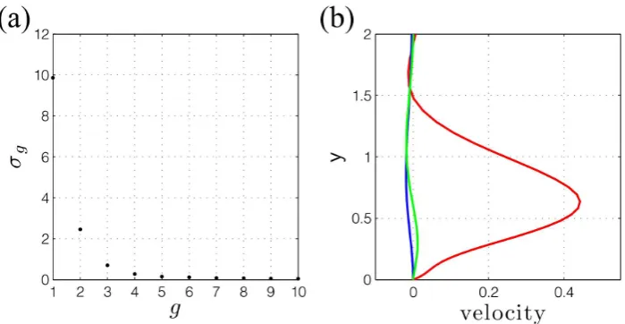
Figure 5. (a) First 10 singular values ofQx¯D, (b) wall-normal variation (real part) of the ˜ux1,nych (red), ˜vx1,nych (blue), and ˜wx1,nych (green)
components of the first column of ¯BD.
in whichU1∈Cm×g, Σ1∈Rg×g andg is the number of ‘significant’ disturbance inputs, obtained by inspecting the diagonal elements ofΣ1, shown in Figure 5(a). Based on this Figure, a disturbance model with just two inputs was selected, i.e.g=2. A disturbance input matrix ¯BD∈Cm×gwas then defined as follows:
¯
BD:=U1
p
Σ1. (20c)
Note that ¯BDB¯∗D≈Qx˜D. Of course, the question of whether or not this was the ‘best’ disturbance model
for the purposes of control or estimation is open for debate. The present model was chosen purely on the grounds of convenience and the fact that it is physically plausible. For example, it is interesting to plot the wall-normal variation of the elements of the first column of ¯BD, since this represents the ‘shape’ of the
principal disturbance entering the state. Figure 5(b) shows this variation for the real part of the elements corresponding to ˜ux1,nych, ˜vx1,nych and ˜wx1,nych. As expected, the disturbances are mainly confined to the
boundary layer. The forcing term ¯Bin (19a) was obtained from the following; ¯
B
¯
G
=TBD¯ , (21)
where ¯G∈C(n−m)×gandT is the transformation matrix in (13a).
With respect to measurements, the wall-normal gradients at the wall of the streamwise and spanwise velocities were used, in the sensor location planesx1,x2andx3:
∂ux˜ 1,Nych
∂y (k)
∂wx˜ 1,Nych
∂y (k)
∂ux˜ 2,Nych
∂y (k)
∂wx˜ 2,Nych
∂y (k)
∂ux˜ 3,Nych
∂y (k)
∂wx˜ 3,Nych
∂y (k)
| {z }
yk =
Y1∗0 0 0 0 0 0 0 0 0 0 0 0Y1∗0 0 0 0 0 0 0 0 0 0 0 0Y1∗0 0 0 0 0 0 0 0 0 0 0 0Y1∗0 0 0 0 0 0 0 0 0 0 0 0Y1∗0 0 0 0 0 0 0 0 0 0 0 0Y1∗
| {z }
¯
CD
xDk, (22)
[image:14.595.114.464.53.234.2]the node at the wall). The notationY1∗is to be interpreted as ‘rowNy and all columns of the matrixY1’, and each zero entry is a row vector ofNyzeros. The output equation (19b) was formed as follows:
yk=C¯DS
xk zk
+vk= [C¯ H¯]
xk zk
+vk
=Cx¯ k+Dw¯ k+vk. (23)
where ¯H ∈Cp×(m−n) and ¯D:=−H¯G¯ (Sch¨on et al. 2003). Note that, although difficult to obtain ex-perimentally, wall-shear stress information was employed in this study since this is sufficient to enable estimation of the flow-field above the wall, at least in the linear (transient growth) case (Bewley and Protas 2004).
Thus, with all terms in (19) defined, a discrete-time-varying Kalman filter (Franklin et al. 1997, p. 391) was synthesised for the system. Note that this filter produces estimates ˆxk, but it is straightforward
to interpret these states in terms of the velocities and pressures in ˆxDk via the transformation:
ˆ
xDk=S
ˆ
xk
ˆ
zk
. (24)
whereSis the transformation matrix in (13a). The results are described in the next section.
7 Results and Discussion
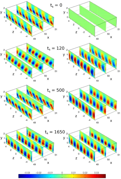
The streamwise velocity perturbation fields above each of the sensing locations are shown in Figure 6 for the initial and three subsequent sample times. It should be noted that the initial state of the estimator is zero. Clearly, the Kalman filter, employing a low-order, linear model of the Navier-Stokes equations, a noise model with only two stochastic inputs, and measurements obtained solely from wall shear in-formation, is reconstructing the characteristic streaky disturbances within the transient growth region of the boundary layer. It should be noted that the estimated streaks are of approximately the correct shape, location and magnitude, despite uncertainty in the initial conditions. Thus, the main aim of this paper is achieved.
Quantitatively, the estimates differ slightly from the DNS data. Figures 7, 8 and 9 shows the estimated versus actual streamwise velocity components at three different heights above the wall (and within the boundary layer) in the central streamwise sensing plane. As is to be expected, as distance above the wall (where the sensors are located) increases, so too does the error between the estimates and the DNS data.
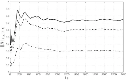
Convergence of the Kalman Filter was deduced by studying the convergence of the variance-related quantitykRk2,y,[0k], where R:w∗k v∗k∗ 7→xˆDk,y,u−xDk,y,u, for k∈[0 Nk]. Here, ˆxDk,y,u denotes the
es-timate of a streamwise velocity Fourier component at a particular height above the wall. The quan-titykRk2,y,[0k]was defined as follows:
kRk2,y,[0k]:=
v u u t1
k k
∑
n=0 n
ˆ
xDk,y,u−xDk,y,u
∗ ˆ
xDk,y,u−xDk,y,u
o
. (25)
Figure 10 shows a plot of this quantity against sample timetk askis increased from zero toNk =1201, for the three different heights in Figures 7, 8 and 9. This plot clearly shows that the variance of the error between estimates and DNS data is lower closer to the wall, and also suggests convergence fortk'1000.
Figure 7. Real and imaginary parts of the streamwise velocity perturbations ˜ux at a height above the wall ofy=0.23. Actual velocity components are shown in blue, whilst estimates are shown in red.
Figure 8. Real and imaginary parts of the streamwise velocity perturbations ˜ux at a height above the wall ofy=0.35. Actual velocity components are shown in blue, whilst estimates are shown in red.
[image:17.595.62.517.50.299.2] [image:17.595.63.519.345.599.2]Figure 9. Real and imaginary parts of the streamwise velocity perturbations ˜uxat a height above the wall ofy=0.69 (streak-centre height). Actual velocity components are shown in blue, whilst estimates are shown in red.
Figure 10. Variance related measure versus sample time of streamwise velocity Fourier components at heightsy=0.69 (solid line),y=0.35 (dashed line) andy=0.23 (dashed dotted line).
[image:18.595.62.519.51.300.2] [image:18.595.84.489.345.602.2]week of wall-clock time on 96 processors of the HLRB-II Supercomputer to compute. Even the transient growth region, which is computationally less expensive, requires significant computational resources to compute. This is in stark contrast with the real-time speed at which the current Kalman Filter computes estimates.
Finally, it should be noted that in the present study the Kalman Filter employed a noise model de-rived directly from the DNS data of the entire flow-field. However, in practice it is more likely that one would only possess a small sub-set of this data, provided by sensor based measurements. Future work may therefore attempt to construct a noise model from measurement data alone (Odelson et al. 2006, Rajamani and Rawlings 2009).
8 Conclusions
Motivated by the problem of drag reduction via flow control, this paper began with the Navier-Stokes Equations and employed a series of modelling approximations to yield a linear, low-order state-space model describing disturbance evolution within the transient growth region of a boundary layer. Using this model, together with DNS-based wall shear measurements, a Kalman filter was synthesised that reproduced the characteristic streaky disturbances that are known precursors of turbulence, and hence increased skin-friction drag. Such a model could easily be used for closed-loop controller synthesis. Furthermore, it was argued that the numerical method described in this paper, for converting a system of DAEs into an equivalent system of ODEs, significantly reduced the modelling burden by allowing straightforward satisfaction of boundary conditions whilst dispensing with the need for commonly em-ployed parallel-flow assumptions and velocity-vorticity transformations.
Given the complexity of the underlying system, the limited measurements and the simplicity of both the model and the estimator, the velocity-field estimates were very encouraging. Future work could focus on integrating wall actuators as part of a complete closed-loop feedback scheme within the existing DNS of the flow, and also deriving noise models solely from measurement data.
Acknowledgements
The authors would like to thank Ahmed Naguib, Philippe Lavoie, Ati Sharma and Bharath Ganapathisub-ramani for many fruitful discussions on boundary layer estimation.
References
Aamo, O.M., and Krstic, M.,Flow control by feedback: Stabilization and Mixing, Springer (2003). Andersson, P., Berggren, M., and Henningson, D.S. (1999), “Optimal disturbances and bypass transition
in boundary layers,”Physics of Fluids, 11, 134–150.
Arg¨uelles, P., Bischoff, M., Busquin, P., Droste, B.A.C., Evans, R., Kr¨oll, W., Lagard`ere, J., Lina, A., Lumsden, J., Ranque, D., Rasmussen, S., Reutlinger, P., Robins, R., Terho, H., and Wittl¨ov, A. (2001), “Meeting Society’s Needs and Winning Global Leadership - European Aeronautics: A Vision for 2020; Report of the Group of Personalities,” Technical report, Office for Official Publications of the European Committee.
Arthur, G.G., McKeon, B.J., Dearing, S.S., Morrison, J.F., and Cui, Z. (2006), “Manufacture of micro-sensors and actuators for flow control,”Microelectronic Engineering, 83, 1205–1208.
Bagheri, S., Brandt, L., and Henningson, D.S. (2009), “Input-output analysis, model reduction and con-trol of the flat-plate boundary layer,”J. Fluid Mech., 620, 263–298.
Baker, J., Myatt, J., and Christofides, P.D. (2002), “Drag reduction in flow over a flat plate using active feedback control,”Computers and Chemical Engineering, 26, 1095–1102.
Bewley, T.R., and Liu, S. (1998), “Optimal and robust control and estimation of linear paths to transi-tion,”Journal of Fluid Mechanics, 365, 305–349.
Bewley, T.R., and Protas, B. (2004), “Skin friction and pressure: the “footprints” of turbulence,”Physica D, 196, 28–44.
Boyd, J.P. (1999), “The Blasius Function in the Complex Plane,”Experimental Mathematics, 8, 381– 394.
Butler, K.M., and Farrell, B.F. (1992), “Three-dimensional optimal perturbations in viscous shear flow,”
Phys. Fluids A, 4, 1637–1650.
Cathalifaud, P., and Bewley, T.R. (2004), “A noncausal framework for model-based feedback control of spatially developing perturbations in boundary-layer flow. Part I: formulation,”Systems and Control
Letters, 51, 1–13.
Chughtai, S.S., and Werner, H. (2010), “Transient Energy Analysis of Spatially Interconnected Model for 3D Poiseuille Flow,” inProceedings of the American Control Conference, June-July, Baltimore, Maryland.
Dai, L.,Singular Control Systems, Lecture Notes in Control and Information Sciences, Springer-Verlag (1989).
Ferziger, J.H., and Peri´c, M.,Computational Methods for Fluid Dynamics, Springer (1997).
Franklin, G.F., Powell, J.D., and Workman, M.,Digital Control of Dynamic Systems, 3rd ed., Addison-Wesley (1997).
Gad-el-Hak, M.,Flow control: Passive, Active and Reactive Flow Management, Cambridge University Press (2000).
Gerdin, M. (2006), “Identification and Estimation for Models Described by Differential-Algebraic Equa-tions,” Link¨oping University, Sweden.
Golub, G.H., and Van Loan, C.F.,Matrix Computations, third ed., The Johns Hopkins University Press (1996).
Hanifi, A., Schmid, P.J., and Henningson, D.S. (1996), “Transient growth in compressible boundary layer flow,”Physics of Fluids, 8, 826–837.
Hoepffner, J., and Brandt, L. (2008), “Stochastic approach to the receptivity problem applied to bypass transition in boundary layers,”Physics of Fluids, 20, 024108.
Hoepffner, J., Chevalier, M., Bewley, T.R., and Henningson, D.S. (2005), “State estimation in wall-bounded flow systems. Part 1. Perturbed laminar flows,”Journal of Fluid Mechanics, 534, 263–294. Hogberg, M., Bewley, T.R., and Henningson, D.S. (2003), “Linear feedback control and estimation of
transition in plane channel flow,”J. Fluid Mech., 481, 149–175.
Jones, B.L., and Kerrigan, E.C. (2010), “When is the discretization of a spatially distributed system good enough for control?,”Automatica, 46, 1462–1468.
Leib, S.J., Wundrow, D.W., and Goldstein, M.E. (1999), “Effect of free-stream turbulence and other vortical disturbances on a laminar boundary layer,”Journal of Fluid Mechanics, 380, 169–203. Luenberger, D.G. (1978), “Time invariant descriptor systems,”Automatica, 22, 312–321.
McKernan, J., Whidborne, J.F., and Papadakis, G. (2007), “Linear Quadratic Control of Plane Poiseuille Flow - the Transient Behaviour,”International Journal of Control, 80, 1912–1930.
Naguib, A.M., Morrison, J.F., and Zaki, T.A. (2010), “On the relationship between the wall-shear-stress and transient-growth disturbances in a laminar boundary layer,”Physics of Fluids, 22, 054103. Odelson, B.J., Rajamani, M.R., and Rawlings, J.B. (2006), “A new autocovariance least-squares method
for estimating noise covariances,”Automatica, 42, 303–308.
Rajamani, M.R., and Rawlings, J.B. (2009), “Estimation of the disturbance structure from data using semidefinite programming and optimal weighting,”Automatica, 45, 142–148.
Reinschke, J., and Smith, M.C. (2003), “Designing robustly stabilising controllers for LTI spatially dis-tributed systems using coprime factor synthesis,”Automatica, 39, 193–203.
Rosenfeld, M., Kwak, D., and Vinokur, M. (1991), “A fractional step solution method for the unsteady in-compressible Navier-Stokes equations in generalized coordinate systems.,”Journal of Computational
Physics, 94, 102–137.
Schmid, P.J. (2007), “Nonmodal Stability Theory,”Annual Review of Fluid Mechanics, 39, 129–162. Sch¨on, T., Gerdin, M., Glad, T., and Gustaffson, F. (2003), “A modeling and filtering framework for linear
implicit systems,” inProceedings of the 42nd IEEE Conference on Decision and Control, December, Maui, Hawaii, USA, pp. 892–897.
Shahzad, A., Jones, B.L., Kerrigan, E.C., and Constantinides, G.A. (2011), “An efficient algorithm for the solution of a coupled Sylvester equation appearing in descriptor systems,”Automatica, 47, 244– 248.
Sturzebecher, D., and Nitsche, W. (2003), “Active cancellation of Tollmien-Schlichting instabilities on a wing using multi-channel sensor actuator systems,”International Journal of Heat and Fluid Flow, 24, 572–583.
Trefethen, L.N.,Spectral Methods in Matlab, SIAM (2000).
Trefethen, L.N., Trefethen, A.E., Reddy, S.C., and Driscoll, T.A. (1993), “Hydrodynamic stability with-out eigenvalues,”Science, 261.
Vaughan, N.J., and Zaki, T.A. (2011), “Stability of zero-pressure-gradient boundary layer distorted by unsteady Klebanoff streaks,”Journal of Fluid Mechanics, In Press.
Weideman, J.A.C., and Reddy, S.C. (2000), “A MATLAB Differentiation Matrix Suite,”ACM
Transac-tions on Mathematical Software, 26, 465–519.
White, F.M.,Fluid Mechanics, McGraw Hill (2003).
Zaki, T.A., and Durbin, P.A. (2005), “Mode interaction and the bypass route to transition,”Journal of
Fluid Mechanics, 531, 85–111.
Zaki, T.A., and Durbin, P.A. (2006), “Continuous mode transition and the effects of pressure gradient,”
Journal of Fluid Mechanics, 563, 357–388.
Zaki, T.A., and Saha, S. (2009), “On shear sheltering and the structure of vortical modes in single and two-fluid boundary layers,”Journal of Fluid Mechanics, 626, 111–147.
Appendix A: Submatrices of (11)
The submatrices ofADnoBCsin(11)are defined as follows:
A1,1:=−
∂Ux1,nych
∂x −Vx1,nychY1+
3
2∆xUx1,nych+
Y2−β2
R ,
A1,2:=−
∂Ux1,nych
∂y , A1,5:=−
2
∆xUx1,nych,
A1,9:= 1
∆xUx1,nych, A2,1:=−
∂Vx1,nych
∂x ,
A2,2:=−
∂Vx1,nych
∂y −Vx1,nychY1+
3
2∆xUx1,nych+
Y2−β2
R ,
A2,4:=−Y1,A2,6:=− 2
∆xUx1,nych, A2,10:=
1
A3,3:=−Vx1,nychY1+
3
2∆xUx1,nych+
Y2−β2
R ,
A3,4:=−iβI,A3,7:=− 2
∆xUx1,nych, A3,11:=
1
2∆xUx1,nych,
A4,1:=−
1
∆xI, A4,2:=
1
2Y1, A4,3:= 1 2iβI,
A4,5:= 1
∆xI, A4,6:=
1
2Y1, A4,7:= 1 2iβI,
A5,1:= 1
2∆xUx2,nych, A5,6:=−
∂Ux2,nych
∂y ,
A5,5:=−
∂Ux2,nych
∂x −Vx2,nychY1+
Y2−β2
R ,
A5,9:=−
1
2∆xUx2,nych, A6,2:=
1
2∆xUx2,nych,
A6,4:=−
1
2Y1, A6,5:=−
∂Vx2,nych
∂x ,
A6,6:=−
∂Vy2,nych
∂x −Vx2,nychY1+
Y2−β2
R ,
A6,8:=−
1
2Y1,A6,10:=− 1
2∆xUx2,nych, A7,3:=
1
2∆xUx2,nych,
A7,4:=−
1
2iβI, A7,7:=−Vx2,nychY1+
Y2−β2
R ,
A7,8:=−
1
2iβI, A7,11:=− 1
2∆xUx2,nych, A8,1:=−
1 2∆xI,
A9,1:=− 1
2∆xUx3,nych, A9,5:=
2
∆xUx3,nych,
A9,9:=−
∂Ux3,nych
∂x −Vx3,nychY1−
3
2∆xUx3,nych+
Y2−β2
R ,
A9,10:=−
∂Ux3,nych
∂y ,A10,2:=
1
2∆xUx3,nych,
A10,6:= 2
∆xUx3,nych, A10,8:=−Y1, A10,9:=−
∂Vx3,nych
∂x ,
A10,10:=−
∂Vx3,nych
∂y −Vx3,nychY1−
3
2∆xUx3,nych+
Y2−β2
R ,
A11,3:=−
1
2∆xUx3,nych, A11,7:=
2
∆xUx3,nych, A11,8:=−iβI,
A11,11:=−Vx3,nychY1−
3
2∆xUx3,nych+
Y2−β2