warwick.ac.uk/lib-publications
Original citation:
Nahian, Syed Abu, Truong, Dinh Quang, Chowdhury, Puja, Das, Debdatta and Ahn, Kyoung
Kwan. (2016) Modeling and fault tolerant control of an electro-hydraulic actuator.
International Journal of Precision Engineering and Manufacturing, 17 (10). pp. 1285-1297.
Permanent WRAP URL:
http://wrap.warwick.ac.uk/87077
Copyright and reuse:
The Warwick Research Archive Portal (WRAP) makes this work by researchers of the
University of Warwick available open access under the following conditions. Copyright ©
and all moral rights to the version of the paper presented here belong to the individual
author(s) and/or other copyright owners. To the extent reasonable and practicable the
material made available in WRAP has been checked for eligibility before being made
available.
Copies of full items can be used for personal research or study, educational, or not-for profit
purposes without prior permission or charge. Provided that the authors, title and full
bibliographic details are credited, a hyperlink and/or URL is given for the original metadata
page and the content is not changed in any way.
Publisher’s statement:
“The final publication is available at Springer via
http://dx.doi.org/10.1007/s12541-016-0153-2
“
A note on versions:
The version presented here may differ from the published version or, version of record, if
you wish to cite this item you are advised to consult the publisher’s version. Please see the
‘permanent WRAP url’ above for details on accessing the published version and note that
access may require a subscription.
NOMENCLATURE
Ah = head side piston area
Ar = rod side piston area
Av = valve opening area
Cv = valve discharge coefficient
D = pump displacement
s k
d
= position sensor fault information of EHA Emax = the bulk modulus of the hydraulic fluidfrc = friction force between cylinder wall and piston Fload = applied load on the cylinder
l = cylinder length m = piston mass
N = pump rotation per minute (RPM) P1 = pump pressure
Ph = head side pressure
Pr = rod side pressure
Prel = relief valve settling pressure
ρ = hydraulic fluid density Qpump = pump flow rate
Vc = control voltage of the servo motor
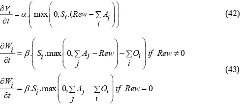
xp = cylinder piston position
Q1 = inlet flow rate to the cylinder
Q2= outlet flow rate from the cylinder
Qrel = flow rate through relief valve
1. Introduction
Electro hydraulic actuators are one of the widely accepted solutions in modern industries. With a wide range of applications like heavy duty excavation or the precise operations like computerized numerical control, it has been considered as a potential choice owing to its compact size, high power to weight ratio and small power consumption. For an example, highly efficient EHAs from Moog, Inc. (East Aurora, New York) were validated in real time simulators in terms of accuracy and fast response [1]. In addition, Rahmfeld and Ivantysynova [2] derive the effectiveness of EHAs mathematically. Such especial features increase the popularity of EHAs over the electric motor driven
Modeling and Fault Tolerant Control of an
Electro-Hydraulic Actuator
Syed Abu Nahian
1,Dinh Quang Truong
1Puja Chowdhury
1Debdatta Das
1, andKyoung Kwan Ahn
2,#1 Graduated School of Mechanical Engineering, University of Ulsan, Daehakro 93, Namgu, Ulsan, South Korea,680-749 2 School of Mechanical Engineering, University of Ulsan, Daehakro 93, Namgu, Ulsan, South Korea,680-749 # Corresponding Author / E-mail: [email protected], TEL: +82-52-259-2282 , FAX: +82-52-259-1680
KEYWORDS :
Electro-hydraulic actuator, Sensor fault, Fault tolerant control, Unknown input observer, BELBIC
In the modern industry, electro-hydraulic actuators (EHAs) have been applied to various applications for precise position pressure/force control tasks. However, operating EHAs under sensor faults is one of the critical challenges for the control engineers. For its enormous nonlinear characteristics, sensor fault could lead the catastrophic failure to the overall system or even put human life in danger. Thus in this paper, a study on mathematical modeling and fault tolerant control (FTC) of a typical EHA for tracking control under sensor-fault conditions has been carried out. In the proposed FTC system, the extended Kalman-Bucy unknown input observer (EKBUIO) -based robust sensor fault detection and identification (FDI) module estimates the system states and the time domain fault information. Once a fault is detected, the controller feedback is switched from the faulty sensor to the estimated output from the EKBUIO owing to mask the sensor fault swiftly and retains the system stability. Additionally, considering the tracking accuracy of the EHA system, an efficient brain emotional learning based intelligent controller (BELBIC) is suggested as the main control unit. Effectiveness of the proposed FTC architecture has been investigated by experimenting on a test bed using an EHA in sensor failure conditions.
actuators in current era. Despite the benefits of the EHAs, these are one of the critical nonlinear systems. It is a challenge for control engineers to control nonlinear systems under varieties of working environments and loads. The system performances are then depended on the adaptability of the controller, and especially the reliability of the sensors.
In a closed-loop control system, faults could be raised either in sensors or actuators. For instance, in sophisticated plants like power plants, chemical process plants, fatal accident may occur due to system fault [3, 4]. Subsequently, with the development of smart machines and systems, safe operations and diagnosis of the malfunctions with desirable performances are becoming important aspects with time. Therefore, researchers have been showing interests to develop fault diagnosis algorithm (FDA) in various applications in recent years [5-9]. In parallel, by adopting control laws with the FDA, one can realize the FTC for any system.
In general, the FTC is a control methodology that ensures the safe operation under acceptable limit of a system when faults occur under FDI system. The FDI problem consists of two sub modules: binary decision making (fault detection) and finding the time variant fault behavior (fault identification). Several procedures were conducted by different researchers for fault detection mechanisms. Chi and Zhang [10] proposed a fault detection method based on failure and non-failure hypothesis of an aircraft system. Parameter estimation is also a way for fault detection [11]. This is done by measuring the input and output signals if the basic model structure is known. Then the process follows direct estimation or numerical optimization. In another case, passive robust fault detection was presented by Puig and Quevedo [12] by bounding the uncertainties in intervals, known as ‘interval model’. Process model-based fault detection was also evaluated using residual analysis [13]. Meanwhile, observer-based fault identification was carried out by different researchers [14, 15]. These conducted researches reflect the effectiveness of the FDI in fault tolerant control systems.
In today’s industry, sensor fault is one of the most important issues that could be occurred at any time without screening any previous symptoms. Especially, a process operated by a nonlinear EHA has potential probability of occurring sensor faults due to high operating pressures or tough working environments or even external impacts on the sensors. For example, sensor faults could be happened in accelerometers of aircraft [16], position sensors [13], sensors in heavy duty tele-operated demolition or excavation robots or hydraulic press load cells due to fatigues, fluctuations of hydraulic fluid, external impacts on sensors or human errors. Such failures lead the controllers to produce wrong control signals which may degrade significantly the overall performances or even put the
human life in endanger. Therefore, sensor FTC is becoming one of the firing issues in modern control of EHAs.
In sensor FTC architecture, evaluation of redundant sensor systems is generally used in most of the applications. For an example, Chan and Hong [17] successfully showed how to classify faults under noise using redundant sensors and a modified kohonen network. Furthermore, linear sensor redundancy analysis-based FTC has been recently carried out by Santhosh [18]. In commercial EHAs like VariStroke-I from Woodward (USA), redundant linear displacement transducers have been used for FTC operation. However, the sensor redundancy increases the hardware and FDI designing complexity as well as cost, weights, maintenance effort. Therefore, researchers focused the spot light on the analytical redundancy over hardware redundancy for designing FTC architectures. For an instance, analytical redundancy-based fault diagnosis method by developing a filter with sequential probability ratio test was proposed by Chi and Zhang [10]. In an EHA positioning system, such FTC was carried out by Navid and Nariman [19]. They developed quantitative feedback-based FTC module in which the system was identified by single-input-single-output transfer function. However, the identification of such nonlinear systems with this manner is not feasible. Also, they could not reveal the fault information invoked at the sensors.
Intelligent approaches, like fuzzy, genetic algorithm (GA) and neural network, have been found for FTC in EHA applications. FTC of an electro hydraulic servo axis was studied by Beck and Mark [13] with fuzzy logic-based fault diagnosis. Mendonca and Sousa [20] presented a multiple fuzzy fault model-based FTC and verified it through simulations of a three-tank hydraulic system. Although the simulated fault diagnosis performance was feasible, the excessive fuzzy-based fault model with high degree of expert knowledge as well as large number of parameters increased the computational complexity. Later on, Shang [21] proposed an intelligent fault classification method based on GA and back propagation technique applied to a transmission system. This employed an improved genetic search with fast Fourier transformation (FFT) to solve high dimensional feature selection problem with low computational complexity. Nevertheless, the system vibration and speed signals were required for spectral transformation that involved lots of experimental tests.
detects, isolates and identifies the sensor faults effectively. However in most cases, these researches were conducted without practical verification and sensor/process noises were omitted while large categories of the real systems are stochastic. The extended Kalman filter (EKF) can be a good solution to deal with the stochastic system. Haldar [28] showed a procedure to detect and isolate the sensor fault of an EHA system using conventional EKF. However, the time domain fault information could not be revealed with this approach.
From the above analysis, this paper develops an effective sensor fault tolerant control for an EHA-driven cylinder. The main objective is to control precisely the cylinder position while additive or multiplicative fault is invoked in the system sensors during operation. The FTC architecture is designed with two modules: FDI module and main control module. An unknown input observer adopting with extended Kalman-Bucy filter, called EKBUIO, is proposed as the FDI module. This module takes part in estimating the system states and the unknown input: sensor fault. Using the estimated time domain fault information, threshold-based decisions are then made for fault detection in the EHA system. In order to control the system effectively, an adaptive and computationally efficient online brain emotional learning-based intelligent controller (BELBIC) has been suggested as the main control module. The architecture is realized on the model to mimic those parts of the brain which are known to produce emotion [29]. Consequently being different from the conventional closed-loop architecture having only single control module, the proposed FTC approach possesses both the adaptive control solution and robust fault tolerant methodology to meet the requirement of an effective EHA control performance under sensor faults. An EHA apparatus is setup and, the experimental investigation has been carried out in order to validate the effectiveness of the FTC system in faulty conditions.
This paper is sketched as follows: in Section 2, the overall description of the EHA apparatus has been introduced at first. Then the mathematical modeling of the test bed and the system parameter estimation are studied in Section 3. In Section 4, the developed FTC controller with trajectory control strategy is discussed comprehensively. The experimental investigations are carried out in Section 5 to evaluate the effectiveness of the proposed FTC system applied into EHA. Finally, the conclusion is drawn in Section 6.
2. EHA Apparatus
In this section, the outline of the overall EHA setup is presented.
M
m
Tank chamber Effective chamber Valve chamber Valve 1
Valve 3 Valve 2
Valve 4
Chamber 1 Chamber ch
Chamber cr
pump
Q
1
Q Q2
rel
Q
NI PCI 6221
Servo Driver
Computer
[image:4.595.307.551.64.243.2]Linear sensor
Fig. 1 Configuration of the EHA test rig
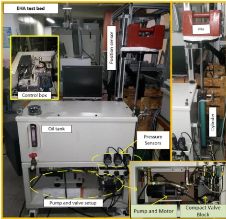
Fig. 1 shows the system configuration. As seen in Fig. 1, the EHA system includes hydraulic cylinder driven by a three-phase servo motor and a hydraulic pump with one direction and fixed displacement through a hydraulic valve circuit. This valve circuit consists of four high-speed ON/OFF solenoid controlled valves and one safety pressure regulating valve to perform all operations of the cylinder. The advantages of using a four-valve configuration, such as velocity control or energy saving, has been clearly presented by Shenouda [30]. By this concept, the pressurized flow from the pump can be transmitted to the cylinder to follow the desired tasks by smoothly selecting five modes [30].
In this study, only cylinder power extraction (PE) and power retraction (PR) modes are considered for developing the FTC approach. A personal computer (PC) with compatible specifications
[image:4.595.313.543.516.739.2]
0 2 4 6 8 10 12
0 1 2 3 4 5
0 1 2 3 4 5
0 1 2 3 4 Measured dP (bar) Flow (lpm) a) b) measured estimated Cv
Pressure drop (bar)
Fig. 3 a) dP-Q curve b) Cv-dP curve
3. System modeling and identification
3.1 System modeling
The mathematical modeling of the EHA described in the previous section is elaborated in this part. As the valves and servo motor are fast in response, the dynamics are assumed to be linear for the sake of simplicity. The pump flow rate can be calculated as
pump
s c
Q DN
N k V
(1)
where: ks is a proportional parameter, which defines the RPM to
voltage ratio of the servo motor. Now, the momentum equation is
( )
p h h r r load
mx A P A P F frc (2)
Theoretically, the bulk modulus Emax is the ratio of the change
in pressure to the fractional change in volume of any chamber and
can be assumed as its mean value given common pressures and
temperatures. However in practice, this can be substantially lowered
by entrained gas and mechanical compliance. In this study (Fig. 1),
it can be represented as a sensitive pressure-domain function [31].
By considering the entrained air and mechanical compliance, the
empirical effective bulk moduli of the divided chambers,
c1,
ch and
crare computed as7 1 7
7
(0.4 2 10 ) 1 max
(0.4 2 10 ) max
(0.4 2 10 ) max (1 ) (1 ) (1 ) h r P c P ch P cr E e E e E e
(3)
The flows and continuity equations through the circuit can be expressed as (4) and (5) respectively [32].
1
1 1
1
1 1 1 1
2 2
2 3 3
1
4 4 1
2 | | ( ) 0
2 | |
( )
2 | | ( ) 2 | |
( )
2 | |
( )
vr v rel
rel
h
v v h
h
v v h
r
v v r
r
v v r
P
c A sign P if P P
Q
otherwise
P P
Q a c A sign P P
P
a c A sign P
P
Q a c A sign P
P P
a c A sign P P
(4)
1 1 1 1 1 2 2 1 2 ( ( ) ( )) ( ) cpum p rel
c
pump rel
h ch
p h
ch p h
r ch
p r
cr p r
dP
a Q Q Q
dt V
a Q Q Q
dP
Q x A
dt V x A
dP
x A Q
dt V l x A
(5)
where:
Vc1
,
V
ch,
V
cr are the internal constant pipe volumes of‘Chamber 1’, ‘Chamber ch’ and ‘Chamber cr’ respectively and
1 3 2 4 1 3 2 4 1; 1 0 0; 0 0; 0 0 1; 1 p p a a x a a a a x a a
Assuming that the valve discharge coefficients
cv1=cv2=cv3=cv4=Cv are the same, due to the same valve
configuration. Certainly, this coefficient Cv is dependent on the flow
dynamics of the valve including flow conditions, laminar or turbulent,
deferential pressure, dP, valve opening area,Av and fluid density.
For the sake of simplicity, the fluid density can be taken as a
constant and because of using high-speed ON/OFF solenoid
controlled valves in the EHA, the effect of changing valve area is
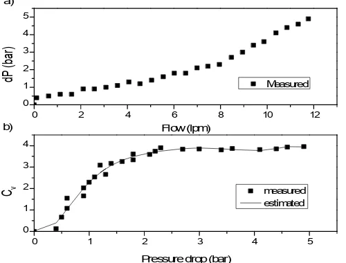
considered very low and can be neglected as well. Thus the Cv is
defined by investigating the relationship between the pressure drop,
dP, and flow rate, Q, of each valve as presented in Fig. 3(a). The
tendency of Cv over dP is then illustrated as Fig. 3(b) and, finally,
approximated by a polynomial function using interpolation technique [33] as follows
2 7 1 6 5 4
3 2 2
1.100 10 +2.040 10 1.5263 5.8795
12.17865832 12.146 2.204 1.890 10
v
C dP dP dP dP
dP dP dP
(6)
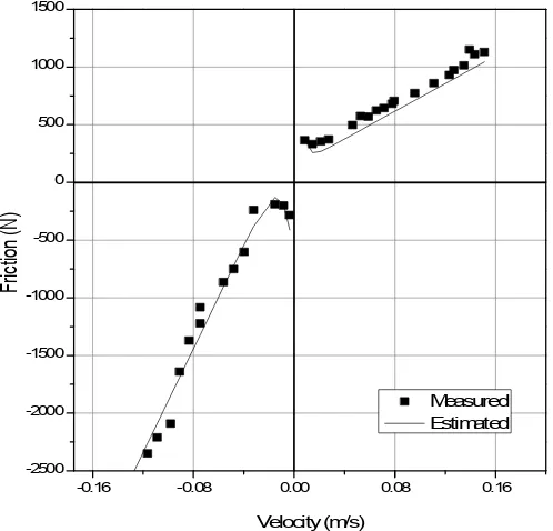
The friction load presented in (2) can be modeled as [31],
( )( ) 0
( )( ) 0
p su p sd x C
u p p cu su p
x C
d p p cd sd p
x Sign x F F e x
frc
x Sign x F F e x
[image:5.595.43.293.55.245.2]-0.16 -0.08 0.00 0.08 0.16 -2500
-2000 -1500 -1000 -500 0 500 1000 1500
Measured Estimated
Friction (N)
Velocity (m/s)
[image:6.595.43.292.63.302.2]
Fig. 4 Friction force vs. cylinder speed.
here: uanddare the viscous friction parameters; Fcu and Fcd are
the coulomb frictions; Fsu and Fsd are the static friction forces ; Csu
and Csd are known as Stribeck velocity parameters for the ‘up’ and
‘down’ motion of the cylinder, respectively. Subsequently, based on the dynamic equations from (1) to (7), the system can be
represented by a state vector
1 2 3 4 5 1
[ ]T [ ]T
p p h r
x x x x x x x P P P and can be expressed as
1 4 2 5 1
1 2
1 1
3 1 1 2 2
1 1
4
1 2 1 5
2 1
2 1 2 2 1
1
( )
0 0
( )
0
( 1000)
1000 0
( 1000 )
( ) * *1000
c c
pump
ch
h
cr
r
A x A x frc
m x
x x
x a Q a Q Q
V V
x
Q x A
x
V x A
A x Q
V l x A
(8)
From (8), it can be seen that the presented EHA is the complex
system with nonlinear dynamic terms. Moreover, as the developed
FTC scheme (see Section 4) relies on the extended Kalman-Bucy
filter, the state estimation performance can get advantages from the
system description with minimal modeling error. Thus, it is
necessary to derive the accurate model. The system parameters can
be found either from the manufacture provided datasheet or can be
identified experimentally. In this paper, the observed and known
terms are listed in Table 1. On the other hand, some unobserved
Table 1 EHA physical parameters
Components values Unit
Ah 0.00126 m
2
Ar 0.00088 m2
Av 2.54 10 6 mm2
D 16.3 cm3
Fload 20 Kgf
m 0.43 Kg
Emax 1.5 10 9 Pa
870 Kg/m3Prel 40 bar
l 500 mm
Table 2 Optimized model parameters
Parameters Identified values Unit
Vc1 0.1996 L
Vch 0.0394 L
Vcr 0.201 L
u
5915.8 Ns/m
d
22554 Ns/m
Fcu 28.62 N
Fcd 364.02 N
Fsu 774.12 N
Csu 0.00012 m/s
Csd 0.007541 m/s
ks 300 RPM/V
terms like the chamber volumes, friction coefficients, valve parameters and RPM to voltage ratio parameter can be derived by performing a parameter optimization procedure which is discussed in the next subsection.
3.2 Parameter estimation
Here, the unobserved parameters were estimated by offline tuning method with Matlab/Simulink parameter estimation toolbox.
First based on the friction-velocity relationship (Fig. 4) derived from the experiments, the friction parametersu,d, Fcu, Fcd, Fsu,
Fsd, Csu and Csd were identified. Next, with the identified friction
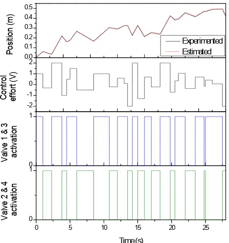
model, the constant volumes, Vc1, Vch, Vcr and the proportional
parameter ks were estimated based on a random set of input/output data of the EHA. Fig. 5 displays the comparison between the model output and actual response of the cylinder corresponding to arbitrary input signals of the motor and valves. This result shows that the model with optimized parameters could represent well the actual system
[image:6.595.42.287.399.600.2]
0.0 0.1 0.2 0.3 0.4 0.5
-2 -1 0 1 2
0 1
0 5 10 15 20 25
0 1
Position (m)
Experimented Estimated
Control effort
(V)
Valve 1 &
3
activation
Valve 2 &
4
activation
[image:7.595.50.284.48.296.2]Time (s)
Fig. 5. Comparison between model output and actual system response.
k
r e f
k
y
ˆk
y
s k
d
Fig. 6 Position control configuration of EHA with sensor FTC
4 FTC design for EHA
The proposed FTC system for EHA system has been demonstrated in Fig. 6. In operation, the BELBIC acts as the main controller and performs conventional closed-loop trajectory control. Once the fault detection is made (See Section 4.2) the decision is to switch the feedback from between the sensor and the estimated position output of the EKBUIO using an operator defined as a ‘flag switch’. Hence, the sensor fault can be masked and the controller reconfiguration is not required which is a complicated procedure to retain system stability. The design procedures of each module of the FTC system are discussed in next subsections.
4.1 Extended Kalman-Bucy Unknown Input Observer
For a generic system, the unknown input is an undefined time variant characteristic with unbounded amplitude that can be experienced by either sensor or actuator which leads the system
instability. Therefore in this paper fault is considered as an unknown input and in this section, the design procedure of unknown input observer based on the extended Kalman-Bucy filter (EKBF) is explained elaborately.
At first, a simple unknown input observer is derived for a linear time invariant system with a form of
x Ax Bu
y Cx
(9)
where: n, m, r
xR yR uR are system state vector, output vector, input vector. , ,A B C are the known matrices with proper dimensions corresponding to linear, time invariant system state space description. Now in discrete form, the linear system with actuator unknown input and additive noises could be derived as [15]
1
k k k k k k k k
x A x B u E d w (10)
k k k k
y C x v (11)
where: n, m, r, q
k k k k
x R y R u R d R are discrete time system state vector, output vector, known input vector, unknown input vector representing as fault respectively.w vk, kare the zero mean
white noise and A,
k k k
A e B B and C Care calculated for discretization purpose with
sampling time.Considering the unknown input observer in form of
1 1 1 1
k k k k k k k k
z Fz TB u K y (12)
1 1 1 1
ˆk k k k
x z H y (13)
where: ˆ 1 , zk+1
n n
k
x R R are the estimated state vector and states of the observer. The observer matrixesFk1,Tk1,Hk1 and Kk1
should be designed in a way that the state estimation error k+1 k+1 ˆk1
e x x asymptotically converses to zero. From (10) to (13), the error term can be derived as
1
k+1 1 1 1 1 1 1
2
1 1 1 1 1 1
1
1 1 1 1 1 1 1
[ ( ) ]
[ ] [ ( )]
( ) ( )
k k k k k k k k k
k k k k k k k k k
k k k k k k k k k k k
e F I H C A K C x F e
K F H y T I H C B u
I H C E d H v I H C w K v
(14)
where: 1 2
1 1 1
k k k
K K K . Therefore to form the UIO, the following relations must hold.
1 1
k k k k
E HCE (15)
1 1 1
1 1 1 1 1 2
1 1 1
k k k
k k k k k
k k k
T I H C
F T A K C
K F H
(16)
The necessary and sufficient conditions for the observer of the given system are [34]:
[image:7.595.49.282.339.454.2]Subsequently, one special solution of (15) could be obtained as
1 1 1 1 1
1 1 1
1 1 1 1 1 1 1
( )
[( ) ] ( )
k k k
k k k
T T
k k k k k k
H E H
H C E
C E C E C E
(17) Thus, the state estimation error becomes: 1
1 1 1 1 1 1
k k k k k k k k k
e
F e
K v
H v
T w
(18) It is obvious that without additional noises and disturbances, ek+1 will converse to zero asymptotically if Fk+1 is stable. So, inorder to design the observer, one has to select the stable Fk+1 by a
proper choice of 1 1
k
K . Another study [35] shows that to derived ek+1
with minimum variance the gain matrix can be written as
1 1
1 1 [ ]
T T
k k k k k k k k k
K T A P C C P C R
(19)
where: the covariance matrices are given by
1 1 1/ 1, 1 1 1 1 1 1
1
1/ 1 1
T T T
k k k k k k k k k k k k k k k k k k k k
P T A P A T Q T H R H
P P K C P T A
(20)
Now, the observer can be converted into Kalman filter form in order to estimate the states in the stochastic environment. Now, multiplying (11) with 1
1
k
H and inserting in (10) leads
1
1[ 1 1( ˆ )]
k k k k k k k k
d H y C A x B u (21)
From (10) and (21), one has
1 1
k k k k k
x Ax Bu E y (22)
where:
k k k
A G A,BkG Bk 1
1 1,
k k k k
G I E HC
1 1
k k k
E E H
Consequently the unknown input observer for the linear system can be given as [36]
1 1 1/ 1
ˆk ˆk k k ( k kˆk)
x x K y C x (23)
where:
1/ 1
k k k k k k
x Ax Bu E y (24)
Secondly for a nonlinear discrete time invariant system, Witczac and Pretki [37] developed an extended unknown input observer based on EKF algorithm. Let the system is defined as
1 ( ) ( )
k k k k k k
x g x h u E d W (25)
1 1 1
k k k k
y Cx V (26)
where: Wk~(0,Q Vk), k~(0,Rk),k are independent and (.), (.)
g h are nonlinear functions. The extended UIO can be expressed as
1
1 1/ 1 1 1/
ˆk ˆk k k ( k kˆk k)
x x K y C x (27)
Similarly, by multiplying 1 1
k
H with (26) and solving with (25)
leads the unknown input as
1
1[ 1 1( ( ) ( ))]
k k k k k k
d H y C g x h u (28)
By substituting with (25), the prior state can be estimated as
1/ 1
ˆk k ( )ˆk ( )k k k
x g x h u E y (29)
where:
(.) k (.),
g G g h(.)G hk (.)
1 1 1,
k k k k
G I E H C
1 1
k k k
E E H
The error covariance matrixes and the Kalman gain can be calculated as
1/
T k k k k k k
P A P A Q (30)
1 1
1 1/ 1( 1 1/ 1 1)
T T
k k k k k k k k k
K P C C P C R
(31)
1
1 [ 1 1] 1/
k k k k k
P IK C P (32)
where: ˆ | ( ) ( ) k k k k
k k k k
k k x x
g x g x
A G G A
x x
In the above mathematical derivation, the unknown input dk can be considered as an actuator unknown input. Consequently, in order to find the sensor unknown input: the fault in the EHA system position sensor, a subsequent procedure is followed. The nonlinear EHA system is modeled as
( ) ( ( )) ( ( )) ( )
k k k
x t f x t b u t W t
y Cx V
(33)
where: f(.) and b(.) are the nonlinear functions corresponding to (8) and the observation with the unknown sensor fault with fault distribution matrix Em can be modeled as
( ) ( ) ( )
s k k m k k s s
y Cx E d V
d t d t t
(34)
Here, ( )t is the auxiliary unknown input. Now to design the proposed EKBUIO of the EHA system, consider the augmented system state space representation becomes into
( ( )) ( ( ))
( )
( ) ( ( )) ( ( )) 0 ( ) 0 1 ( ) ( ) [ ] t k s s E h u t g X t
X t
k m k
C
x t f x t b u t
t d t
d t
y C E X
(35)
Then, using the form of (29) to (32), the predict and time update equations of the EKBUIO can be formulated as follows
ˆ( ) (ˆ( )) ( ( )) ( ) ( ) ( ) ( )
t
T a
c c c
X t g X t h u t E y t
P t A P t P t A Q
(36)
1 1| 1 1 1| 1 1 1| 1
ˆ( ) ˆ ( ) ( )
k k k
k k k
k k k
X t X
P t P
y t y
ˆ ( )
1
ˆ ˆ
( ( )) ( ( )) ˆ
( ) ( )
[( ) ] ( )
c k
X t
t t t
T T
t k t k t k t
g X t g X t
A G
X t X t
E E H
H C E C E C E
HereXˆkand Pkis the estimated states and the corresponding error
covariance matrix of the system presented on (35) at time k. The Kalman gain and covariance matrices are derived by
1
| 1 | 1 | 1
| 1
( ) , ( )
( )
T T
k k k k k k k k k k k k
k k k k k
K P C C P C R P P t
P I K C P
(37)
Finally, the estimated states are calculated as
| 1 | 1 | 1
ˆ ˆ ( ˆ ), ˆ ˆ( )
k k k k k k k k k k k
X X K y C X X X t (38)
4.2 Fault detection technique
In general fault diagnosis mechanism, a system fault is detected
by evaluating fault information (set of sensor data, estimated
unknown fault, etc.) through which ‘fault detection’ decision is made.
Then the decision expression is conveyed as a Boolean indicator and
defined as a fault flag
0,1 . For each fault flag, a recovery action has to be taken in order to avoid system instability. In this paper, theEKBUIO is implemented for sensor fault detection based on the
estimation of fault information ‘ s k
d ’. Indeed, this estimated
information s k
d carries an unknown additive magnitude of the fault
invoked in the sensor at each time step k. Consequently, memory and
computational problems due to dealing with a vast amount of
sensor/process data in probabilistic approach [38] or signal processing
approach [39] can be avoided in the proposed fault detection
technique.
It is obvious that, s k
d should be zero when the sensor is out of the
fault and the fault flag is set to zero. A decision of ‘sensor fault’ is
made by triggering the fault flag=1 while| s| 0
k
d . However in
practice, modeling error, system uncertainty or un-modeled
environment phenomenon are also considered as the unknown input
in the sensor and may interfere with the estimation performance (the
estimated error would be affected, (see (18)). These impacts are then
reflected through the estimated s k
d and directly affect the fault flag
handling. Therefore in order to reduce this influence, a simple but
effective solution is suggested by comparing s k
d with a threshold
value
to set the fault flag as follows:
fault flag=1 if| s|
k
d ( non-zero positive constant)
fault flag=0 otherwise
The value of the threshold
is defined based on the system andenvironment characteristics. It needs to be selected carefully to cover
only the modeling error and system uncertainties. If this threshold is
too tight, a false alarm can be triggered not only by the original sensor
fault, but also the modeling error or environmental influences (e.g.
electro-magnetic interferences). On the other hand, if it is set to too
large, original fault would be hidden. For both cases, the control
performance can be degraded or suffers from instability. Hence, in
our study, the reasonable value of
has been selected based on trial-and-error method by investigating the system performance with its
different settings. The selection procedure as well as the influence of
different settings of
on the system performance is clearly describedin Section 5.1.3.
4.3 BELBIC controller design
In this paper, one of the recent innovated psycho-biological motivated brain emotional learning based intelligent controller (BELBIC) has been used for tracking control of EHA. Recent conducted researches [40, 41] revealed that how efficiently BELBIC can handle nonlinearities and uncertainties under noise and disturbances in EHA applications. The presented controller configuration is mainly based on a typical brain emotional model illustrated in Fig. 7.
In short, there are four main components in the BEL system. According to study [29], there are some Sensory inputs Si entering into Thalamus (Fig. 7(a)). In Thalamus, some simple pre-processes, such as noise reduction, are done [39]. Then the signals are sent to Amygdala and Sensory cortex. The Sensory inputs enter to Orbitofrontal cortex (OFC) as well. There is a digital memory type loop connection between Amygdala and OFC. Finally, the model output is produced by Amygdala. Fig 7(b) represents the detailed configuration of these four blocks. In Amygdala, there exists a relationship between sensory inputs by a plastic and a learning path to each node ‘ ’. There is an additional node connected to Thalamus, is the maximum quantity of the Sensory inputs that is
max( )
th i
S S (39)
Amygdala output Ai and OFC output Oi are calculated by (40) and
(41), respectively. i i i
AS V (40)
i i i
O
SW
(41)Fig. 7 General structure of a Brain Emotional Model (BEL)
t
( )
e t u t( )
( )
r y t
[image:10.595.45.289.386.492.2]Fig. 8 BELBIC architecture for EHA position control
Here, the plastic weights of the Amygdala Vi and OFC Wi are
evaluated by an associative learning system like Rescorla-Wagner model of learning:
. max 0, .(
i
i V
S Rew Ai
t i
(42)
. .max 0, 0
. .max 0, 0
j i
j i
Wi S A Rew O if Rew
i
t j i
Wi S A O if Rew
i
t j i
(43)
Here, Aj are all the Amygdala nodes except the Thalamus node;
and are the learning rates of Amygdala and Orbitofrontal cortex individually; Rew is the ‘Reward’ function. Finally, the model output can be derived:
i i
E A O
i i
(44)
The ‘max ’ functions in (42) ensures the Amygdala’s monotonic learning. That is, once the emotional reaction is learned, it should be permanent. The OFC inhibits the inappropriate behavior of Amygdala. The OFC learning rule is similar to the Amygdala rule except that the plastic weights of this sector can increase and decrease.
In order to be used the BEL model as the controller – BELBIC, the reward function and Sensory inputs should contain some feedback signals, which are generally defined as
( , , ) ( , , , )
i p
i p r
Rew J S e y
S f u e y y
(45)
Illustration from (45), the reward function and Sensory inputs ‘ ’ could be arbitrary functions of the reference input , control input , error and plant output . In common, a proper set of these functions and their weights are selected in order to increase the control performance [40].
5. Experiments
In this section, real-time experiments with tracking control of the
EHA presented in Section 2 in faulty condition has been carried out to
evaluate the designed FTC approach (Fig. 6) including the fault
identification, fault detection and biologically inspired control
(BELBIC). The control design procedure and verification process
are then presented as bellows.
5.1 Experiment setting and control parameter design
5.1.1 BELBIC setting
To utilize the BELBIC for EHA tracking control, its structure is built as shown in Fig. 8. For designing the BELBIC as the main control module, the sensory inputs were carefully chosen as
180 3 20 i
r e
S u dt
y
(46)And the reward function can be selected as a formation of proportional-integral-derivative control form [40]. In this study, it was set as
100 4 0.2de
Rew e e dt
dt
(47)The learning rates were then selected as 0.0000003and 0.000002
for Amygdala and OFC respectively.
5.1.2 EKBUIO setting
The designed EKBUIO, expressed by from (33) to (38) in Section 3, observes the system pressure and position signals, P1, Ph,
Pr and yk. The measurement matrix C and the fault distribution
matrix Em in (36) can be written as
0 0 0 0 0
0 1 0 0 0
0 0 1 0 0
0 0 0 1 0
0 0 0 0 1
C
and 0 1 0 0 0
m
E
0.0 0.2 0.4 0.6 0.8 1.0
-1.2 -0.6 0.0 0.6 1.2
-0.04 -0.02 0.00 0.02 0.04
0 5 10 15 20
0 1
0.01
Reference True Position with True Position with
Position (m)
Hidden Fault
1.2
Est
imated Fault information
Un-modelled Effects
1.2
0.01
Fault Flag
Time (s)
1.2
0.01
a)
0.00 0.12 0.24 0.36 0.48 0.60
0 5 10 15 20
-0.04 -0.02 0.00 0.02 0.04
Position (m)
Reference True Position
0.03 opt
Fault
in
formation
Time (s)
Estimated (EKBUIO) Interferences b)
Fig. 9 System performance analysis: a) with different values ofb)
with optimal value of
10 12 10 10 10 7 2 2 2 2 2
( 10 10 10 10 10 2.25 10
( .001 .015 2 2 2 )
a c
k
Q diag
R diag
5.1.3 Fault detection threshold setting
In order to distinguish between the original invoked fault and the
un-modeled effects on the system, the fault detection threshold value
was determined carefully by the experiment-based trial-and-error
method. It is to be mentioned that, played an important role in this
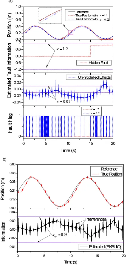
FTC performance. Fig. 9a shows an analysis of the effect of the
threshold values on the system tracking results using the proposed
FTC. With the large value, 1.2, the FTC mechanism had low sensitivity. Thus, the system could track well the desired trajectory
[image:11.595.309.551.49.174.2]only when there was no fault existing.
Fig. 10 Simulink control system using the proposed FTC
When the fault appeared, it was covered by the threshold value and
the fault flag was not triggered. Subsequently, the system suffered
from instability for this missed alarm (see the red-dash lines in the
first, second and fourth sub-plots). On the other hand, with a small
setting of 0.01the FTC mechanism was set to higher sensitivity. In this case, the system tracking performance was degraded. The
reason was that the estimated fault information of the EKBUIO
frequently passed the threshold value even there were only impacts of
un-modelled terms. This, subsequently, resulted many wrong fault
flags (see the blue-dot lines in the first, third and fourth sub-plots).
In order to find the optimum value of, firstly the fault flag=0 was set, and then the system trajectory was controlled by the main
controller under no-fault condition (See the first sub-plot of Fig. 9b).
The estimated fault information can be observed as displayed in Fig.
9b (See the second sub-plot). As seen, it was bounded under 0.03 m,
and 0.03was set in order to suppress this effect.
Finally, the designed control architecture was built in the Simulink environment combined with Real-time Windows Target
toolbox of MATLAB as shown in Fig. 10. It has been then validated on the EHA systems in two faulty conditions: additive sensor fault case and multiplicative sensor fault case. Furthermore, a comparative study with a typical BELBIC closed-loop control (without FTC function) was also performed to clarify the ability of the proposed approach. The sampling period was set to 0.001 s for all experiments.
5.2 Experiment results
5.2.1 Control under additive sensor fault
For the first faulty case, the system was tested to track a sinusoidal trajectory with 0.7 Hz frequency and 0.4m amplitude under the additive sensor fault as depicted in Fig. 11. Here, additive fault was invoked into the controller feedback signal from time t=15
[image:11.595.63.276.54.497.2]0.00 0.38 0.76 1.14
0.00 0.12 0.24
0.0 0.5 1.0 1.5
0 2 4 6 8 10 12 14 16 18 20 22
-2 0 2 4 6
Position (m)
Reference
Faulty sensor respons (without FTC) Estimated Position True position (with FTC) True position (without FTC)
Fault masking activated
Error (m)
True error (with FTC) True error (without FTC)
Fault
information
Invoked fault Estimated fault
Time (s) Control effort (V)
Control effort without FTC Control effort with FTC
Fig. 11 Trajectory control with additive sensor fault
0.00 0.25 0.50 0.75 1.00
-0.4 -0.2 0.0 0.2
-0.4 -0.2 0.0 0.2 0.4
0 2 4 6 8 10 12 14 16 18 20 22
-3 -2 -1 0 1 2 3
Position (m)
Reference
Faulty sensor response (without FTC) Estimated position
True position (with FTC) True position (without FTC)
Fault masking activated
Error (m)
True error (with FTC) Estimated position error Transitional error True error (without FTC)
Fault invoking error
Fault
information (m)
EKBUIO estimated fault magnitude
Control effort (
V)
Time (s) Control effort with FTC
Control effort without FTC
[image:12.595.56.277.58.327.2]
Fig. 12 Trajectory control with multiplicative sensor fault
However due to the lack of FDI ability, this controller could not retain the performance when existing any fault (as shown in the first and second sub-plots of Fig. 11 with the cyan-dash-dot-dot line and red-dash line, respectively). Without the FTC, the BELBIC got the wrong position information and subsequently, generated the wrong
control effort which caused the system to be unstable with large tracking error. On the contrary by using the proposed control approach, the tracking performance was always kept in the acceptable range even existing any fault. It can be see that the control error in this case was only changed slightly when the fault happened (see the black-solid line in the second sub-plot). The reason is that the proposed method possesses not only the adaptability of the BELBIC module but also the sensor fault masking capability of the EKBUIO-based FDI module. The fault estimation result and control effort of this FTC method were in turn shown in the third and fourth sub-plots.
5.2.2 Control under multiplicative sensor fault
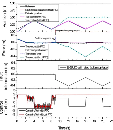
Next, the experiments with the second faulty case were then carried out. Here, a saw signal in the first sub-plot of Fig. 12 was used to represent the desired trajectory. The fault was generated by setting the position sensor gain to zero at t=9 s. Thus the sensor response to be zero suddenly and the position sensor can be considered as 100% failed (as shown in the first sub-plot of Fig. 12
with the red-dash-dot-dot line). Similarly to case 1, with the existence fault, the BELBIC without FTC architecture, could not be able to track the reference. Nevertheless, the designed FTC method still enhanced the acceptable tracking performance even facing fault (see black-solid line and the cyan-dash-dot-dot line of the third sub-plot respectively). Moreover, the estimated fault information of EKBUIO and good control effort of using this method are showed in the third and fourth sub-plots of Fig. 12
respectively.
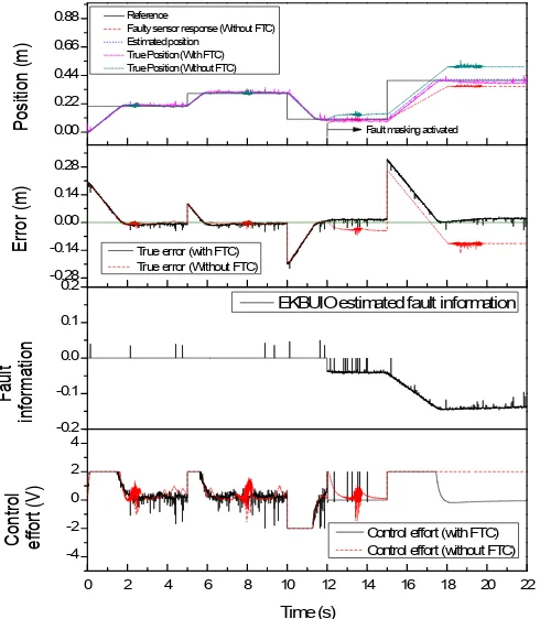
Finally, the experiments were carried out with a multi-step tracking reference in the second faulty case. As the results obtained in Fig. 13, the fault was invoked by setting the sensor gain with 0.7 at t=12 s. That is the sensor was assumed to be degraded 30% of its current value (see the red-dash line of the first sub-plot of Fig. 13). With and without the FTC, the BELBIC tracks the trajectory in similar fashion. Meanwhile without the FTC system, the control error also degraded 30%. Because, the main control module could not have any fault information (see the red-dash line of second sub-plot). On the other hand, with FTC, the fault was detected quickly and continued the tracking operation with an acceptable accuracy (see the second sub-plot with black-solid line). The estimated fault information of the EKBUIO and the optimal control effort requirements are figured in the third and fourth sub-plots respectively (see the black-solid lines in each of the sub-plot).
[image:12.595.49.284.366.638.2]
0.00 0.22 0.44 0.66 0.88
-0.28 -0.14 0.00 0.14 0.28
-0.2 -0.1 0.0 0.1 0.2
0 2 4 6 8 10 12 14 16 18 20 22
-4 -2 0 2 4
Position (m)
Reference
Faulty sensor response (Without FTC) Estimated position
True Position (With FTC) True Position (Without FTC)
Fault masking activated
Error (m) True error (with FTC) True error (Without FTC)
Fault
information
EKBUIO estimated fault information
Time (s)
Control effort
(V)
Control effort (with FTC) Control effort (without FTC)
[image:13.595.45.290.50.331.2]
Fig. 13 Trajectory control under sensor performance degradation
6. Conclusions
In this paper, the fault tolerant control approach has been developed for tracking control of an electro-hydraulic actuator under sensor fault conditions. The proposed FTC is successfully designed as the combination of the main control module, BELBIC, and the fault detection and identification module. Here, the BELBIC is designed as a trajectory controller. Meanwhile, the EKBUIO-based FDI module estimates the system states and the unknown fault information.
In order to investigate the practical effectiveness of the developed FTC architecture, real-time experiments with position tracking control of the researched EHA using this logic have been carried out in case of existing additive and multiplicative sensor fault conditions. In addition, the comparative study with the BELBIC controller without FDI function was also performed to validate the advance of the proposed control method. The experimental results implied that the BELBIC controller could ensure the precise and stable performance when tracking the desired profiles in the normal working condition. However when facing with the faulty problems, only the suggested FTC architecture with the advanced design of the FDI module could retain the system stability. Meanwhile, the stability was totally degraded when using the conventional closed-loop system without this module. Our
future research topics will be carried out on partial-model and non-model based robust fault tolerant control in different EHA driven
industrial applications.
ACKNOWLEDGEMENT
This work was supported by the Technology Innovation Program (10043810, Development of a 20~40kW smart hybrid power pack for industry based on intelligent control) funded By the Ministry of Trade, Industry & Energy(MI, Korea) and by the Human Resource Training Program for Regional Innovation and Creativity through the Ministry of Education and National Research Foundation of Korea (NRF-2015H1C1A1035547).
REFERENCES
1. Kim, M.Y. and Lee, C.O. “An Experimental Study on The Optimization of Controller Gains For An Electro-Hydraulic Servo System Using Evolution Strategies,” J. of Control Engineering Practice, Vol. 14, pp. 137-147, 2006.
2. Rahmfeld, R. and Ivantysynova, M. “Displacement Controlled Linear Actuator With Differential Cylinder – A Way to Save Primary Energy in Mobile Machines,” In: Proceedings of The 5th International Conference on Fluid Power Transmission and Control, pp.316 –3 22 , 2001.
3. Zarei, J., and Shokri, E., “Robust Sensor Fault Detection Based on Nonlinear Unknown Input Observer,” Measurement, Vol. 48, pp. 355-367, 2014.
4. Pierri, F., Paviglianiti, G., Caccavale, F., and Mattei, M., “Observer-Based Sensor Fault Detection and Isolation for Chemical Batch Reactors,” Engineering Applications of Artificial Intelligence, Vol. 21, No. 8, pp. 1204-1216, 2008. 5. R., Petersen, I., and C., McFarlane, D., “A Methodology for
Robust Fault Detection in Dynamic Systems,” J. of Control Engineering Practice, Vol. 12, pp. 123-138, 2004.
6. Hashemi, A., and Pisu, P., “Fault Diagnosis in Automotive Alternator System Utilizing Adaptive Threshold Method,” In: Proceedings of The Prognostics and Health Management Society, 2011.
7. F., Odgaard, P., and Stoustrup, J., “Unknown Input Observer Based Detection of Sensor Faults In A Wind Turbine,” In: Proceedings of The IEEE International Conference on Control Applications, pp. 310-315, 2010.