Minimum Distance Estimation of Search Costs using Price Distribution

City, University of London Institutional Repository

Citation

: Sanches, F., Silva Junior, D. & Srisuma, S. (2016). Minimum Distance

This is the accepted version of the paper.

This version of the publication may differ from the final published

version.

Permanent repository link:

Link to published version

: http://dx.doi.org/10.1080/07350015.2016.1247003

Copyright and reuse:

City Research Online aims to make research

outputs of City, University of London available to a wider audience.

Copyright and Moral Rights remain with the author(s) and/or copyright

holders. URLs from City Research Online may be freely distributed and

linked to.

City Research Online: http://openaccess.city.ac.uk/ [email protected]

Minimum Distance Estimation of Search Costs

using Price Distribution

y

Fabio Sanches

University of São Paulo

Daniel Silva Junior

City University London

Sorawoot Srisuma

University of Surrey

September 9, 2016

Abstract

Hong and Shum (2006) show equilibrium restrictions in a search model can be used to

identify quantiles of the search cost distribution from observed prices alone. These quantiles

can be di¢ cult to estimate in practice. This paper uses a minimum distance approach to

estimate them that is easy to compute. A version of our estimator is a solution to a nonlinear

least squares problem that can be straightforwardly programmed on softwares such as STATA.

We show our estimator is consistent and has an asymptotic normal distribution. Its distribution

can be consistently estimated by a bootstrap. Our estimator can be used to estimate the cost

distribution nonparametrically on a larger support when prices from heterogeneous markets

are available. We propose a two-step sieve estimator for that case. The …rst step estimates

quantiles from each market. They are used in the second step as generated variables to perform

nonparametric sieve estimation. We derive the uniform rate of convergence of the sieve estimator

that can be used to quantify the errors incurred from interpolating data across markets. To

illustrate we use online bookmaking odds for English football leagues’matches (as prices) and

…nd evidence that suggests search costs for consumers have fallen following a change in the

British law that allows gambling operators to advertise more widely.

JEL Classification Numbers: C13, C15, D43, D83, L13

Keywords: Bootstrap, Generated Variables, M-Estimation, Search Cost, Sieve Estimation

We are very grateful to the authors of Moraga-González, Sándor and Wildenbeest (2013) for sharing their MATLAB code with us. We thank an anonymous referee for helpful comments and suggestions. We would also like to thank

Valentina Corradi, Abhimanyu Gupta, Tatiana Komarova, Dennis Kristensen, Arthur Lewbel, and Paul Schrimpf for some helpful discussions.

1

Introduction

Heterogenous search cost is one of the classic factors that can be used to rationalize price dispersion of homogenous products. E.g., see the seminal work of Stigler (1964). Various empirical models of search have been proposed and applied to numerous problems in economics depending on data availability. Hong and Shum (2006, hereafter HS) show that search cost distributions can be identi…ed from the price data alone. The innovation of HS is very useful since price data are often readily available, for instance in contrast to quantities of products supplied or demanded.

We consider an empirical search model with non-sequential search strategies. HS show the quan-tiles of the search cost in such model can be estimated without specifying any parametric structure. Although there has been more recent empirical works that extend the original idea of HS to estimate more complicated models of search1, there are still interests in the identi…cation and estimation of the simpler search model nonparametrically. For examples, Moraga-González, Sándor and Wildenbeest (2013) show how data from di¤erent markets can be used to identify the search cost distribution over a larger support and Blevins and Senney (2014) consider a dynamic version of the search model we consider here.

The main insight from HS is that the equilibrium condition can be summarized by an implicit equation relating the price and its distribution, parameterized by the proportions of consumers searching di¤erent number of sellers. The latter can be used to recover various quantiles of the search cost distribution. Two main features of the equilibrium condition that lead to an interesting econometric problem are: (i) it imposes a continuum of restrictions since the mixed strategy concept leads to a continuous distribution of price in equilibrium; and, (ii) the observed price distribution is only de…ned implicitly and cannot be solved out in terms of terms of price and the parameters of interest.

In this paper we make two main methodological contributions that complement existing estima-tion procedures and make the empirical search model more accessible to empirical researchers.

First, when there are data from a single market, we provide an estimator for the quantiles on the cumulative distribution (cdf) of the search cost that is simple to construct and easy to perform inference on. Our estimator uses all information imposed by the equilibrium condition. We show under very weak conditions that our estimator is consistent and asymptotically normal at a para-metric rate. We also show the distribution of our estimator can be approximated consistently by a standard nonparametric bootstrap. The ease of practical use is the distinguishing feature of our estimator compared to the existing ones in nontrivial ways. Its simplest version can be obtained by

1_{E.g. see Hortaçsu and Syverson (2004), De los Santos, Hortaçsu and Wildenbeest (2012), and Moraga-González,}

de…ning the distance function using the empirical measure that leads to a nonlinear least squares problem that can be implemented on STATA.

Second, when there is access to data from multiple markets, we propose a two-step sieve estimator that pools data across markets and estimate the cdf of the search cost as a function over a larger support. Single market data can only be used to identify a limited number of quantiles. Our sieve estimator provides a systematic way to combine quantiles from di¤erent individual markets. Any estimator in the literature can be used in the …rst stage, not necessarily the one we propose. The second stage estimation resembles a nonparametric series estimation problem with generated regressor and regressand. We provide the uniform rate of convergence for the sieve estimator. Since we know the rate of convergence of quantiles from each individual market, the uniform rate using pooled data can be used to quantify the cost of interpolation across markets.

For estimation HS takes a …nite number of quantiles, each one to form a moment condition using the equilibrium restriction written in terms of quantiles, and develop an empirical likelihood estimator that has desirable theoretical properties such as e¢ ciency and small …nite sample bias (e.g. see Owens (2001) and Newey and Smith (2004)). However, a …nite selection from in…nitely many moment conditions may have implications in terms of consistent estimation and not just e¢ ciency (Dominguez and Lobato (2004)). Some preliminary algebra suggests such issue may be relevant in the model of search under consideration. But at the same time, with …nite data, it is also not advisable to use arbitrary many moment conditions for empirical likelihood estimation or any other optimal GMM methods due to the numerical ill-posedness associated with e¢ cient moment estimation; see the discussion in Carrasco and Florens (2002). Particularly, a well-known problem with the empirical likelihood objective functions is they typically have many local minima, and the method is generally challenging to program and implement; see Section 8 in Kitamura (2007). Indeed HS also report some numerical di¢ culties in their numerical work; in their illustration they choose the largest number of quantiles that allow their optimization routine to converge.2

Partly motivated by the numerical issues associated with HS’s approach, Moraga-González and Wildenbeest (2007, hereafter MGW) propose an inventive way to construct the maximum likelihood estimator by manipulating the equilibrium restriction. They suggest the likelihood procedure is easier to compute and, importantly, is also e¢ cient. However, the numerical aspect in terms of the imple-mentation of their estimator remains non trivial. The di¢ culty is due to the fact that the probability density function (pdf) of the price is de…ned implicitly in terms of its cdf, the latter in turns is only known as a solution of a nonlinear equation imposed by the equilibrium. This leads to a constrained likelihood estimation problem with many nonlinear constraints. A naïve programming approach to

2_{Hong and Shum (2006) illustrate their procedure using online price data of some well-known economics and}

this optimization problem is to directly specify a nested procedure requiring an optimization routine on both the inner and outer loop, where the inner step searches over the parameter space and the outer step solves the nonlinear constraints. A more numerically e¢ cient alternative may be possible by using constrained optimization solvers with algorithms that deal with the nonlinear constraints endogenously. See Su and Judd (2012) for a related discussion and further references.3

We take a di¤erent approach that is closely related to the asymptotic least squares estimation described in Chapter 9 of Gourieroux and Monfort (1995). Asymptotic least squares method, which can be viewed as an alternative representation to the familiar method of moment estimator, is partic-ularly suited to estimate structural models as the objective functions can often be written to represent the equilibrium condition directly. For examples see the least squares estimators of Pesendorfer and Schmidt-Dengler (2008) and Sanches, Silva Junior and Srisuma (2016) in the context of dynamic discrete games.4 _{However, the statistical theory required to derive the asymptotic properties of our}

estimator in this paper is more complicated than those used in the dynamic discrete games cited above since here we have to deal with a continuum of restrictions instead of a …nite number of restric-tions. We derive our large sample results using a similar strategy employed in Brown and Wegkamp (2002), who utilize tools from empirical process theory to derive analogous large sample results for a di¤erent minimum distance estimator.5

The estimator we propose focuses on the ease of practical use but not e¢ ciency. There are at least two obvious ways to improve on the asymptotic variance of our estimator. As alluded above, the equilibrium restriction can also be stated as a continuum of moment conditions. Therefore an e¢ cient estimation in the GMM sense can be pursued by solving an ill-posed inverse problem along the line of Carrasco and Florens (2000).6 _{It is arguably even simpler to aim for the fully}

e¢ cient estimator. For instance we can perform a Newton Raphson iteration once, starting from our easy compute estimate, using the Hessian from the likelihood based objective function proposed by MGW. Then such estimator will have the same …rst order asymptotic distribution as the maximum likelihood estimator (Robinson (1988)). But, of course, there is no guarantee the asymptotically e¢ cient estimator will perform better than the less e¢ cient one in …nite sample.

3_{An important feature for the search model under consideration is that the number of constraints is large and}

grows with sample size, while many other well-known structural models, such as those associated with dynamic

discrete decision problems and games, have a …xed and relatively small number of constraints.

4_{Pesendorfer and Schmidt-Dengler (2008) also illustrate how a moment estimator can be cast as an asymptotic}

least squares estimator.

5_{They consider a minimum distance estimator de…ned from a criterion based on a conditional independence}

condi-tion due to Manski (1983).

6_{Also see a recent working paper of Chaussé (2011), who is extending the estimator of Carrasco and Florens (2000)}

When the data come from a single market, an inevitable limitation of the identifying strategy in HS is that only countable points of the distribution of the search cost can be identi…ed. Partic-ularly there is only one accumulation point at the lower support of the cost distribution. In order to identify higher quantiles of the cost distribution, and possibly its full support, Moraga-González, Sándor and Wildenbeest (2013) suggest combining data from di¤erent markets where consumers have the same underlying search distribution. In particular they provide conditions under which pooling data sets can be used for identi…cation. In terms of estimation they suggest that interpolating data between markets can be di¢ cult. In order to overcome this, they propose a semi-nonparametric maximum likelihood estimator for the pdf of the search cost. The cdf, which is often a more conve-nient object to make stochastic comparisons, can then be obtained by integration. However, their semi-nonparametric maximum likelihood procedure is complicated as it solves a highly nonlinear optimization problem with many parameters. They show their estimator can consistently estimate the distribution of the search cost where the support is identi…ed but do not provide the convergence rate.7

Building on the semi-nonparametric idea, we propose a two-step sieve least squares estimator for the cdf of the search cost. The estimation problem involved can also be seen as an asymptotic least squares problem where the parameter of interest is an in…nite dimensional object instead of a …nite dimensional one. We show that sieve estimation is a convenient way to systematically combine data from di¤erent markets. It can be used in conjunction with any aforementioned estimation method, not necessarily with the minimum distance estimator we propose in this paper. In the …rst stage an estimation procedure is performed for each individual market. In the second stage we use the …rst-step estimators as generated variables and perform sieve least squares estimation. Our sieve estimator is easy to compute as it only involves ordinary least squares estimation. We provide the uniform rate of convergence for our estimator. The ability to derive uniform rate of convergence is important as it gives us a guidance on the cost of estimation the entire function compared to at just some …nite points, which we know to converge at a parametric rate within each market.

The large sample properties of our sieve estimator are not immediately trivial to verify. In prac-tice our second stage least squares procedure resembles that of a nonparametric regression problem with generated regressors and generated regressands. There has been much recent interest in the econometrics and statistics literature on the general theory of estimation problems involving gen-erated regressors in the nonparametric regression context (e.g., see Escanciano, Jacho-Chávez and Lewbel (2012, 2014) and Mammen, Rothe and Schienle (2012, 2014)). Problems with generated vari-ables on both sides of the equation seem less common. Furthermore, the asymptotic least squares

7_{Details can be found in the supplementary materials to Moraga-González, Sándor and Wildenbeest (2013),}

framework generally di¤ers from a regression model. We are not aware of any general results for an asymptotic least squares estimation of an in…nite dimensional object. However, our problem is somewhat simpler to handle relative to the cited works above since our generated variables converge at the parametric rate rather than nonparametric. We derive the properties for our sieve estimator under the framework that the data have a pooled cross section structure. Our approach to derive the uniform rate of convergence is general and can be used in other asymptotic least squares problems.

We conduct a small scale Monte Carlo experiment to compare our proposed estimators with other estimators in the literature. Then we illustrate our procedures using real world data. We estimate the search costs using online odds, to construct prices, for English football leagues matches in the 2006/7 and 2007/8 seasons. There is an interesting distinction between the two seasons that follows from the United Kingdom (UK) passing of a well-known legistration that allows bookmakers to advertise more freely after the 2006/7 season has ended. We consider the top two English football leagues: the Premier League (top division) and the League Championship (2nd division). We treat the odds for matches from each league as coming from di¤erent markets. We …nd that the search costs generally have fallen following the change in the law as expected.

We present the model in Section 2, and then we de…ne our estimator and brie‡y discuss its relation to existing estimators in the literature. Section 3 gives the large sample theorems for our estimator that uses data from a single market. Section 4 assumes we have data from di¤erent markets; we de…ne our sieve estimator for the cdf of the search cost and give its uniform rate of convergence. Section 5 is the numerical section containing a simulation study and empirical illustrations. Section 6 concludes. All proofs can be found in the Appendix.

2

Model, Equilibrium Restrictions and Estimation

primitives (G; p; r; K); see Moraga-González, Sándor and Wildenbeest (2010). We denote the cdf of the equilibrium price distribution by F. The constancy of the seller’s equilibrium pro…t is our starting point:

(p; r) = (p r)

K

X

k=1

kqk(1 F (p)) k 1

s.t. (p; r) = (p0; r) for all p; p0 _{2 S}P; (1)

where _SP = p; p is the support ofPi for some0< p < p <1, andqk is the equilibrium proportion

of consumer searching k times for1 k K. Once_fqkg K

k=1 are known, they can be used to recover

the quantiles of the search cost distribution from the identity:

qk =

8 > > < > > :

1 G( 1);

G( k 1) G( k);

G( K 1);

fork = 1

fork = 2; : : : ; K 1

for k=K

; (2)

where k =E[P1:k] E[P1:k+1]andE[P1:k]denotes the expected minimum price from drawing prices

fromk i.i.d. sellers, which is identi…ed from the data. For further details and discussions regarding the model we refer the reader to HS, MGW and also Moraga-González, Sándor and Wildenbeest (2010).

The econometric problem of interest in this and the next sections is to …rst estimate_fqkg K

k=1 from

observing a random sample of equilibrium prices _fPig N

i=1, and then use them to recover identi…ed

points of the search cost distribution: _f( k; G( k))g K 1

k=1 . First note that we can concentrate out

the marginal cost by equating (p; r) and p; r ,

r(q) = pq1 p

PK k=1kqk

q1 PK_k=1kqk

: (3)

Following HS, the equilibrium condition for the purpose of estimation can be obtained from equating from (p; r) = (p; r) for all p. In particular, this relation can be written as

p=r(q) + _PK (p r(q))q1 k=1kqk(1 F (p))

k 1 for all p2 SP: (4)

Before we introduce our estimator we now brie‡y explain how the equations above have been used for estimation in the literature.

Empirical Likelihood (Hong and Shum (2006))

Since Pi has a continuous distribution the inverse of F, denoted by F 1, exists so that p =

F 1_{(F (p))for all p. Note that equation (4) is equivalent to}

F (p) = F r(q) + _PK (p r(q))q1 k=1kqk(1 F (p))

k 1

!

Then choose …nite V quantile points, _fslgV_l=1, so that sl 2[0;1]is the sl-th quantile. HS develop an

empirical likelihood estimator of qbased on the following V moment conditions:

h(q;sl) =E

"

sl 1

"

Pi r(q) +

(p r(q))q1

PK

k=1kqk(1 sl)

k 1

##

forl = 1; : : : ; V,

where 1[ ] denotes an indicator function. Clearly one needs to choose V K 1, where the minus one comes from the restriction PK_k=1qk= 1.

In theory we would like to choose as many moment conditions as possible. However, there are practical costs and implementation issues in …nite sample as explained in the Introduction. At the same time, in principle, choosing too few moment conditions can lead to an identi…cation problem. We illustrate the latter point in the spirit of the illustrating examples in Dominguez and Lobato (2004).

Suppose K = 2, and we use q2 = 1 q1, so r(q) =

pq1 p(q1+2(1 q1))

2(1 q1) . For any s0 2 [0;1], the

moment condition becomes:

E

"

s0 1

"

Pi

(p r)q1

q1+ 2 (1 q1) (1 s0)

p p q1 2p(1 q1)

2 (1 q1)

##

,

then for some p0 that satis…es s0 =F (p0), q1 must satisfy

p0 =

p+ pq1 p₂₍₁(q1+2(1_q q1))

1) q1

q1+ 2 (1 q1) (1 F (p0))

p p q1 2p(1 q1)

2 (1 q1)

:

By multiplying the denominators across and re-arranging the equation above, by inspection, it is easy to see we have an implicit function T (q1; p0; F (p0)) = 0 such that, for every pair (p0; F (p0)), T (q1; p0; F(p0))is a quadratic function ofq1. However this suggests there are potentially two distinct

values for q1 that satisfy the same moment condition for a given s0, in which case it may not be

possible give have a consistent estimator for q1 based on one particular quantile.

More generally, whenK >2, eachsl leads to an equation for a general ellipse inRK 1 whose level

set at zero can represent the values of proportions of consumers that satisfy the moment condition associated with each quantile level sl.8 Therefore, with any estimator based on (4), one may be

inclined to incorporate all conditions for the purpose of consistent estimation.

Maximum Likelihood (Moraga-González and Wildenbeest (2007))

Let the derivative of F, i.e. the pdf, by f. By di¤erentiating equation (4) and solve out for f, the implicit function theorem yields:

f(p) =

PK

k=1kqk(1 F (p)) k 1

(p r(q))PK_k=2k(k 1)qk(1 F (p))

k 2 for all p2 SP: (5)

8_{A natural restriction for a proportion can be used to rule out any complex value as well as other reals outside}

MGW suggest a maximum likelihood procedure based on maximizing, with respect toq, the following likelihood function:

e

f(q;p) =

PK

k=1kqk 1 Fe(q;p)

k 1

(p r(q))PK_k=2k(k 1)qk 1 Fe(q;p)

k 2 forp2 SP; (6)

where Fe(q;p) is restricted to satisfy equation (4). In practice supposed the observed prices are

fPigN_i=1. Then for each candidate q0, and eachi, Fe(q0;Pi) can be chosen to satisfy the equilibrium

restriction by imposing that it solves: 0 = Pi r(q0)

(p r(q0_))q0 1

PK

k=1kq0k(1 Fe(q0;Pi))

k 1. However, it may not

be a trivial numerical task to fully respect equation (4). Particularly Fe(q0_;P

i) generally does not

have a closed-form expression and is only known to be a root of some (K 1) th order polynomial. Such polynomial always have multiple roots. The multiplicity issue can be migitated by imposing constraints that Fe(q0;Pi) must be real and take values between 0 and 1, and it must be

non-decreasing in Pi.

Minimum Distance

We propose to use the equilibrium condition directly to de…ne objective functions, rather than posing it as (a continuum of) moment conditions. In particular, in contrast to HS, we use equation (4) without passing the equilibrium restriction through the function F. This approach can be seen as a generalization of the asymptotic least squares estimator described in Gourieroux and Monfort (1995) when there is a continuum of restrictions. It will be also convenient to eliminate the denominators to rule out any possibilities of division near zero that may occur if q1 is close to 0 and papproaches

1. We …rst substituting in for r(q), from (3), then equation (4) can be simpli…ed to:

K

X

k=1

kqk(1 F (p)) k 1

!

(p p)q1 p p

K

X

k=1 kqk

!

=q1 p p

K X k=1 kqk ! :

Next we concentrate out qK in the above equation by replacing it with 1 PK_k=11qk, which leads to

the following restriction:

0 = q1 p p K

K_X1

k=1

(k K)qk

!!

(7)

0

@ K 1

PK 1

k=1 qk (1 F(p))

K 1

+PK_k=11kqk(1 F (p))

k 1

1

A (p p)q1 p p K

K_X1

k=1

(k K)qk

!!

:

this must hold for all p_{2 S}P.

Note that the equation above can be re-written as a polynomial in q K (q1; : : : ; qK 1), which

has qas an argument of the unknown function F; using the empirical cdf to construct the objective function in the latter case introduces non-smoothness in the estimation problem.

3

Estimation with Data from a Single Market

We use the equilibrium restiction (7) to de…ne an econometric model _fm(; )_{g 2} so that m(; ) :

SP !R, where for allp2 SP:

m(p; ) = 1 p p K

K_X1

k=1

(k K) k

!!

(8)

0

@ K 1

PK 1

k=1 k (1 F (p))

K 1

+PK_k=11 k(1 F (p))k 1

1

A (p p) 1 p p K

K_X1

k=1

(k K) k

!!

;

and = ( 1; : : : ; K 1) is an element in the parameter space = [0;1]K 1. We assume the model is

well-speci…ed so that m(p; ) = 0 for all p _{2 S}P when equals q K. Given a sample fPigN_i=1, we

de…ne the empirical cdf as:

FN(p) = 1

N

N

X

i=1

1[Pi p] for all p2 SP:

We then de…ne mN (p; ) as the sample counterpart ofm(p; ) where F is replaced by FN. And we

propose a minimum distance estimator based on

min

2 Z

(mN(p; ))

2

N(dp);

where N is a sequence of positive and …nite, possibly random, measures.

We now de…ne respectively the limiting and sample objective functions, and our estimator:

MN( ) =

Z

(mN(p; ))2 N(dp);

M( ) =

Z

(m(p; ))2 (dp);

b = arg min

2 MN( ):

We shall denote the probability measure for the observed data by _P, and the probability measure for the bootstrap sample conditional on _fPigN_i=1 by P . In what follows we use

a:s:

We adopt the same data generating environment as in HS and MGW.

Assumption A1. _fPigN_i=1 is an i.i.d. sequence of continuous random variables with bounded pdf

whose cdf satis…es the equilibrium condition in (4).

Let 0 denote q K. We now provide conditions for our estimator to be consistent and

asymptot-ically normal.

Assumption A2. (i) m(Pi; ) = 0 almost surely if and only if = 0; (ii) N almost surely

converges weakly to a non-random …nite measure that dominates the distribution of Pi;9 (iii)

R _@

@ m(p; 0) @

@ >m(p; 0) (dp) is invertible.

A2(i) is the point-identi…cation assumption on the equilibrium condition. It is generally di¢ cult to provide a more primitive condition for identi…cation in a general nonlinear system of equations, e.g. see the results in Komunjer (2012) for a parametric model with …nite unconditional moments. Our equilibrium condition presents a continuum of identifying restrictions. A2(ii) allows us to construct objective functions using random measures or otherwise, the domination condition ensures identi…-cation of 0 is preserved. Examples for measures that satisfy A2(ii) include the uniform measure on

SP, in this case N = for all N, and a natural candidate for a random measure is the empirical

measure from the observed data. For the latter, weak convergence is ensured if the class of functions under consideration is Glivenko-Cantelli, which can be veri…ed using the methods discussed in Andrews (1994) and Kosorok (2008). A2(iii) assumes the usual local positive de…niteness condition that follows from the Taylor expansion of the derivative of M around 0.

Theorem 1 (Consistency). Under Assumptions A1, A2(i) and A2(ii), ba:s:_! 0.

Theorem 2 (Asymptotic Normality). Under Assumption A1 and A2,

p

N b 0

d

! N 0; H 1 H 1 ; such that

= Var 2

Z

(p)_B(F(p)) (dp) ; (9)

H = 2

Z

@

@ m(p; 0) @

@ >m(p; 0) (dp); (10)

where _B(F (p))and (p) are de…ned in the Appendix (see equations (16) and (19) respectively).

Given the regular nature of our criterion function, we obtain a root N consistency result as expected. The asymptotic variance ofbcan be consistently estimated using its sample counterparts.

9_{Let D be a space of bounded functions de…ned on S}

P. We say N almost surely converges weakly to a

But this can be a cumbersome task. Speci…cally, althoughH is relatively easy to estimate, requires estimating moments involving (a functional of) a Brownian bridge. Perhaps a more convenient method for inference can be performed base on resampling. Our next result shows the ordinary nonparametric bootstrap can be used to imitate the distribution of bstated in Theorem 2.

Let _fP_igN_i=1 denote a random sample drawn from the empirical distribution from _fPig N

i=1. For

some positive and …nite measure _N, let M_N( ) =R (m_N(p; ))2 _N(dp), wherem_N(p; ) is de…ned in the same way as mN(p; ) but based on the bootstrap sample instead of the original data set. We

can then construct a minimum distance estimator using the bootstrap sample:

b = arg min

2 MN( ): (11)

In addition we require is that N has to be chosen in a similar manner to N. The following statements

are made conditioning on _fPig N i=1.

Assumption A3. _N almost surely converges weakly to N.

A3, as with A2(ii), is not necessary for nonrandom measures (cf. Brown and Wegkamp (2002)). However, it ensures the validity of a fully automated resampling process for instance when the empirical measure is use for _N and _N, with respect to the observed and resampled data.

Theorem 3(Bootstrap Consistency). Under Assumptions A1 to A3, pN b b converges in distribution to _N(0; H 1 H 1) in probability.

Theorem 3 ensures that nonparametric bootstrap can be used to consistently estimate the distri-bution of pN b 0 . Subsequently we can perform inference on 0 via bootstrapping.

By constructionbis the estimator forq K. Then a natural estimator forqK isbK 1

PK 1

k=1 bk.

The large sample properties of bK and the ability to bootstrap its distribution follow immediately

from applications of various versions of the continuous mapping theorem.

Corollary 1 (Large Sample Properties of bK). Under Assumptions A1 and A2: (i) bK a:s:

!qK;

(ii) for some real K >0:

p

N bK qK d

! N(0; 2

K); and with the addition of Assumption A3,

let b_K = 1 PK_k=11b_k where b is de…ned as in (11), then pN b_K bK converges in distribution

to _N(0; 2

K) in probability.

these smooth transformation results are standard, e.g. see Kosorok (2008). Although the asymptotic variances in all three Corollaries can be consistently bootstrapped, for completeness, we also provide their explicit forms in the Appendix.

We next turn to the distribution theory for the estimators of_f kg K 1

k=1 and fG( k)g K 1

k=1. Recall

that k =E[P1:k] E[P1:k+1], so one candidate estimator for k is simply its empirical counterpart.

Alternatively, in order to apply the same type of argument used for Corollary 1, we will employ an alternate identity for k that can be obtained from an integration by parts as shown in MGW (see

equations (7) and (8) in their paper):

k =

Z 1

z=0

w(z;q) [(k+ 1)z 1] (1 z)k 1dz; for k = 1; : : : ; K 1where (12)

w(z;q) = _PKq1(p r(q)) k0=1k0qk0(1 z)

k0 1 +r(q), for z 2[0;1].

In what follows we de…ne bk as the feasible version of k in the above display where w( ;q) is

replaced by w( ;b), and withbK in place ofqK. Therefore bk is necessarily a smooth function of b.

For _fG( k)gKk=11, simple manipulation of equation (2) leads to:

G( 1) = 1 q1; (13)

G( 2) = 1 q1 q2;

..

. = ...

G( K 1) = 1 q1 : : : qK 1:

The above system of equations can also be found in HS (equation A6, pp. 273). We de…ne Gb( k)

by replacingq byb, which is also a smooth function ofb. Therefore the consistency and asymptotic distribution, as well as validity of the bootstrap, for _fbkgK_k=11 and fGb( k)gK_k=11 immediately follow.

Corollary 2 (Large Sample Properties of _fbkgKk=11). Under Assumptions A1 and A2: (i)

b_k a:s:

! k for all k = 1; : : : ; K 1; (ii) for some positive de…nite matrix :

p

N b pN

0 B B @

b1 1

.. .

b_{K 1 K 1}

1 C C A

d

! N(0; ) ;

and with the addition of Assumption A3, let _fb_kgK_k=11 be de…ned using equation (12) where w(z;q)

is replaced by w(z;b ) and b is de…ned in (11), then pN b b converges in distribution to

Corollary 3 (Large Sample Properties of _fGb( k)gKk=11). Under Assumptions A1 and A2: (i)

b

G( k) a:s:

! G( k) for all k = 1; : : : ; K 1; (ii) for some positive de…nite matrix G:

p

N Gb G pN

0 B B @

b

G( 1) G( 1)

.. .

b

G( K 1) G( K 1)

1 C C

A! Nd (0; G) ;

and with the addition of Assumption A3, let _fGb ( k)gKk=11 be de…ned using equation (13) where is

replaced by b , which is de…ned in (11), then pN Gb Gb converges in distribution to _N(0; G)

in probability.

4

Pooling Data from Multiple Markets

In this section we show how data from di¤erent markets can be combined to estimate G. When the data come from a single market, we can only identify and estimate the cost distribution at …nite cut-o¤ points, _f( k; G( k))gK_k=11, since there is only a …nite number of sellers that consumers

can search from (see Proposition 1 in Moraga-González, Sándor and Wildenbeest (2013, hereafter MGSW)). Even if we allow the number of …rms to be in…nite, since k is decreasing in k and

accumulates at zero, we would still not be able to identify any part of the cost distribution above

1 (see the discussion in HS). One solution is to look across heterogenous markets. Proposition 2 in

MGSW provides a su¢ cient set of conditions for the identi…cation ofGover a larger part, or possibly all, of its support based on using the data from di¤erent markets that are generated by consumers who endow the same search cost distribution of consumers but may di¤er in their valuations of the product, and the number of sellers and pricing strategy may also di¤er across markets.

MGSW suggest a semi-nonparametric method based on maximum likelihood estimation to esti-mate the cost distribution in one piece instead of combining di¤erent estiesti-mates of Gacross markets in some ad hoc fashion.10 _{However, it is also quite simple to use estimates from individual markets}

to estimate G nonparametrically in a systematic manner. Here we describe one method based on using a sieve in conjunction with a simple least squares criterion.

Suppose there are T independent markets, where for each t we observe a random sample of prices _fPt

ig Nt

i=1 with a common distribution described by a cdf F

t _{that is generated from the}

prim-itive (G; pt_{; r}t_{; K}t_{). For each market t we can …rst estimate}

fqt kg

Kt

k=1 and use equation (2) to

es-timate _fG( t k)g

Kt

k=1, where fq

t kg

Kt

k=1 and f

t kg

Kt

k=1 are the equilibrium proportions of search and

the corresponding cut-o¤ points in the cost distribution. Proposition 2 in MGSW provides con-ditions where G can be identi…ed on _SC = C; C , where C = limT!1inf1 t T t1 1 and

C = limT!1sup1 t T t1 1. In particular the degree of heterogeneity across di¤erent markets

determines how close _SC is to the full support of the cost distribution.

Recall from (13) that each G( t_k) is expressed only in terms of _fqt_kgK_k=1t , particularly for each t

we have:

G( t₁) = 1 q₁t; (14)

G( t₂) = 1 q₁t q₂t;

..

. = ...

G( t_Kt ₁) = 1 q₁t : : : q_Kt t ₁:

We de…ne the squared Euclidean norm of the discrepancies for this vector of equations when G is replaced by any generic function g that belongs to some space of functions _G by:

t _Wt_{; g =} Kt ₁

X

k=1

1 k

X

k0₌₁

q_kt0

!

g( t_k)

!2 ;

where Wt_{= (q}t

1; : : : ; qKt t ₁; t₁; : : : ; _Kt t ₁). By construction t(Wt; G) = 0. We can then combine

these functions across all markets and de…ne:

T (g) = 1

T

T

X

t=1

t

Wt; g : (15)

The key identifying condition for us is that T(G) = 0. There are other distances that one can

choose to de…ne t, and also di¤erent ways to combine them across markets. We choose this particular functional form of the loss function for its simplicity. Particularly T is just a sum of squares criterion

that is similar to those studied in the series nonparametric regression literature (e.g. see Andrews

(1991) and Newey (1997)) when n1 Pk_k0=1q

t k0

oKt _1;T

k=1;t=1 and f

t kg

Kt _1;T

k=1;t=1 are treated as regressands

and regressors respectively. By using series approximation to estimateGour estimator is an example of a general sieve least squares estimator. An extensive survey on sieve estimation can be found in Chen (2007).

Before proceeding further we introduce some additional notations. For any positive semi-de…nite real matrix A we let (A) and (A) denote respectively the minimal and maximal eigenvalues of

A. For any matrix A, we denote the spectral norm by _kA_k = A>_A 1=2_{, and its Moore-Penrose}

pseudo-inverse by A . We let _G to denote some space of real-valued function de…ned on _SC. We

denote sieves by _fGTg_{T 1}, where GT GT+1 G for any integer T. For any function g in GT,

or in _G, we let _jg_j1 = sup_c2S

Cjg(c)j. For random real matrices VN and positive numbers bN, with

N 1, we de…ne VN =Op(bN)as lim&!1lim supn!1Pr [kVNk> &bN] = 0, and de…ne VN =op(bN)

b2N, the notation b1N b2N means that the ratio b1N=b2N is bounded below and above by positive

constants that are independent of n.

Sieve Least Squares Estimation

We start with the infeasible problem where we assume to know _fWt_gT_t=1. We estimate G

on _SC using a sequence of basis functions fglLg L

l=1 that span GT, where glL : SC ! R for all

l = 1; : : : ; LwithLbeing an increasing integer inT, andLis short forL(T). We usegL_{(c)to denote} (g1L(c); : : : ; gLL(c))>for anyc2 SC, andg = gL( 11); : : : ; gL 1K1 ₁ ; : : : ; gL T₁ ; : : : ; gL T_Kt ₁

>

.

Let denote aPT_t=1(Kt 1) vector of ones, andy= q1₁; : : : ;P_kK₌₁1 1q_k1; : : : ; q₁T; : : : ;PK_k=1T 1q_kT >. Then the least squares coe¢ cient from minimizing the sieve objective function is:

e = g>g g>y:

We denote our infeasible sieve estimator for G byGe, where

e

G(c) =gL(c)>e:

However, we do not observe _fWt

gTt=1. Our feasible sieve estimator can be constructed in two steps.

First step: use the estimator proposed in the previous section we obtainWct_{= (qb}t

1; : : : ;bqKt t ₁;bt₁;

: : : ; bt

Kt ₁) for every t.

Second step: replace(g;y) by(g_b;y_b)where the latter quantities are constructed using _fWct

gT t=1

instead of _fWt

gTt=1. We de…ne our sieve least squares estimator by:

b

G(c) = gL(c)>b; where

b = _bg>_bg g_b>y_b.

Numerically our feasible estimation problem is identical to the estimator from a nonparametric series estimation of a regression function when the regressors and regressands used are based on

fWct

gT

t=1. Notice, however, our sieve estimator is fundamentally di¤erent to a series estimator of a

regression function since we have no regression error and the only source of sampling error (variance) comes from the generated variables we obtain from individual market in the …rst step.

We now state some assumptions that are su¢ cient for us to derive the uniform rate of convergence of Gb.

speci…c; (ii) Pt _{and P}t0

are independent for any t₆=t0_{; (iii) The analog of Assumption A2 holds for}

all markets.

Assumptions B1(i) and B1(iii) ensure that Wct _Wt _=O p 1=

p

Nt _{for allt asN}t

! 1. We

impose independence in B1(ii) between markets for simplicity. In principles the recent conditions employed in Lee and Robinson (2014) to derive the uniform rates of series estimator under a weak form of cross sectional dependence can also be applied to our estimator.

Assumption B2. (i) _fKt

gTt=1 is an i.i.d. sequence with some discrete distribution with support

K= 2; : : : ; K for some K <₁; (ii) _f t

gTt=1 is an independent sequence of random vectors such

that t = t₁; : : : ; t_Kt ₁ is a decreasing sequence of reals, where each variable has a continuous

marginal distribution de…ned on _SC for all t. Furthermore, for any t =6 t0 such that Kt = Kt 0

, t k

and t0

k have identical distribution.

Assumption B2 consists of conditions on the data generating process that ensure any open interval in_SC is visited in…nitely often byf tg

T

t=1 asT ! 1. This allows the repeated observations of data

across markets to nonparametrically identify G on _SC. Note that the size of t is random since

Kt _{is a random variable, so that}

f t

gTt=1 (and thus fW

t

gTt=1) is an i.i.d. sequence. On the other

hand, conditional on _fKt

gTt=1, f

t

gTt=1 is an independent sequence but it does not have an identical

distribution across t. In addition t

k and tk0 are neither independent nor have identical distribution

for a given t. Therefore _f t_kgK_k=1t _;t1₌₁;T is aK dependent process due to the independence across t.

Assumption B3. (i) For K = 2; : : : ; K,

min

1 k K E

h

gL t_k gL t_k >_jKt=Ki > 0; and

max

1 k K E

h

gL t_k gL t_k >_jKt=Ki < ₁;

(ii) There exists a deterministic function (L)satisfying sup_c2S

C g

L_{(c) (L)for all Lsuch that} (L)4L2=T _! 0 as T _{! 1}; (iii) For all L there exists a sequence L = ( ₁; : : : ; _L) _{2 R}L and some >0such that

G gL> L

1=O L :

Assumption B3 consists of familiar conditions from the literature on nonparametric series estima-tion of regression funcestima-tions, e.g. see Andrews (1991) and Newey (1997). B3(i) implies that redundant bases are ruled out, and that the second moment matrices are uniformly bounded away from zero and in…nity for any distribution of t

k under consideration. The bounding of the moments from

distributed sequence of random variables. Assumption B3(ii) controls the magnitude of the series terms. Since Gis bounded, the bases can be chosen to be bounded and non-vanishing in which case it is easy to see from the de…nition of the norm that (L) =O(pL). Some examples for other rates of (L), such as those of orthogonal polynomials or B-splines can be found in Newey (1997, Sections 5 and 6 respectively). Assumption B3(iii) quanti…es the uniform error bounds for the approximation functions. For example if G is s times continuously di¤erentiable and the chosen sieves are splines or polynomials, then it can be shown =s.

Assumption B4. For the same (L) as in B3(ii): (i) for all L and l = 1; : : : ; L, glL 2

GT is continuously di¤erentiable and supc2S_C @gL(c) (L) for all L, and @gL(c) denotes d

dcg1L(c); : : : ; d

dcgLL(c)

>

; (ii) (L) =o pNT as T ! 1, where NT denotes min1 t T Nt.

Assumption B4 imposes some smoothness conditions that allow us to quantify the e¤ect of using generated variables obtained from the …rst-step estimation. B4(i) assumes the bases of the sieves to have at least one continuous derivative that are bounded above by (L). This is a mild condition since most sieves used in econometrics are smooth functions with at least one continuous derivative, even for piece-wise smooth functions where di¤erentiability can be imposed at the knots; see Section 2.3 in Chen (2007) for examples. B4(ii) ensures the upper bound of the basis functions and their derivatives does not grow too quickly over any 1=pNT neighborhood onSC. Note that1=

p

NT is the

rate that max1 t T Wct Wt converges to zero.

Theorem 4 (Uniform rates of convergence of Gb). Under Assumptions B1 - B4, as NT and T

tend to in…nity:

b

G G

1

=Op (L)

h

(L)N_T1=2+L i ,

The additive components of the convergence rate of Gb G

1 come from two distinct sources.

The …rst is the variance that comes from the …rst stage estimation and the latter is the approximation bias from using sieves. The order of the bias term is just the numerical approximation error and is the same as that found in the nonparametric series regression literature. The convergence rate for our variance term is inherited from the rates of the generated variables, which is parametric with respect to NT. Our estimator has no other sampling error. This is due to the fact that, unlike in

a regression context, Wt _{is completely known when}

fqt kg

Kt ₁

k=1 is known hence there is no variance

and well approximated by the product between the derivatives of the basis functions and the sampling errors of the generated variable, which are respectively bounded by (L) and N_T1=2.

The leading term for the uniform convergence rate of Gb depends on whether the sampling error from generated variables across di¤erent markets is larger or smaller than the numerical approxima-tion bias. If (L)N_T1=2 = o(L ), then the e¤ect from …rst stage estimation is negligible for the rate of convergence of the sieve estimator. If, on the other hand the reciprocal relation holds, then the dominant term on the rate of convergence comes from the generated variables.

The uniform rate of convergence in Theorem 4 quanti…es the magnitude for the errors we incur from …tting a curve since the sampling error from point estimation from each market is at most

N_T1=2. However, the asymptotic distribution theory for a sieve estimator of an unknown function is often di¢ cult to obtain and general results are only known to exist in some special cases. We refer the reader to Section 3.4 of Chen (2007) for some details. The development of the distribution theory for our estimator of Gis beyond the scope of this paper.

5

Numerical Section

The …rst part of this section reports a small scale simulation study to compare our estimator with other estimators in the literature in a controlled environment. The second part illustrates our pro-posed estimator using online betting odds data.

5.1

Monte Carlo

We …rst consider the case when the data come from a single market. Here we adopt an identical design to the one used in Section 4.3 of MGW, where they study the small sample properties of their estimator and that of HS. In particular the consumers’search costs are drawn independently from a log-normal distribution with location and scale parameters set at 0:5 and 5 respectively. The other primitives of the model are: (p; r; K) = (100;50;10). We solve for a mixed strategy equilibrium and take 100 random draws from the corresponding price distribution, which can be interpreted as observing a repeated game played by the 10 sellers 10 times. We refer the reader to MGW for the details of the data generation procedure that is consistent with an equilibrium outcome as well as other discussions on the Monte Carlo design.

favorably relative to the empirical likelihood estimator. The comments provided by MGW in this regard are also applicable for our estimator and can be found in their paper. In particular our Tables 1 and 2 can be compared directly with their Tables 3(a) and 3(b) respectively. We also provide analogous statistics associated with the estimator for the cdf of the search cost evaluated at the cuto¤ points in Table 3.

Parameter MLE MDE

True Mean St Dev MSE Mean St Dev MSE

r(q) 50 48:384 4:276 20:896 49:535 3:112 9:900

q1 0:37 0:413 0:111 0:014 0:378 0:114 0:013

q2 0:04 0:043 0:019 0:000 0:039 0:014 0:000 q3 0:03 0:033 0:038 0:001 0:024 0:021 0:001 q4 0:03 0:025 0:046 0:002 0:021 0:028 0:001 q5 0:03 0:025 0:066 0:004 0:027 0:031 0:001 q6 0:02 0:038 0:096 0:009 0:031 0:031 0:001 q7 0:02 0:041 0:110 0:012 0:029 0:027 0:001

q8 0:02 0:050 0:131 0:018 0:025 0:024 0:001 q9 0:02 0:059 0:141 0:022 0:020 0:019 0:000 q10 0:42 0:274 0:239 0:079 0:404 0:158 0:025

Table 1: Properties of maximum likelihood (MLE) and minimum distance (MDE) estimators for

r(q) and q1; : : : ; q10.

Parameter MLE MDE

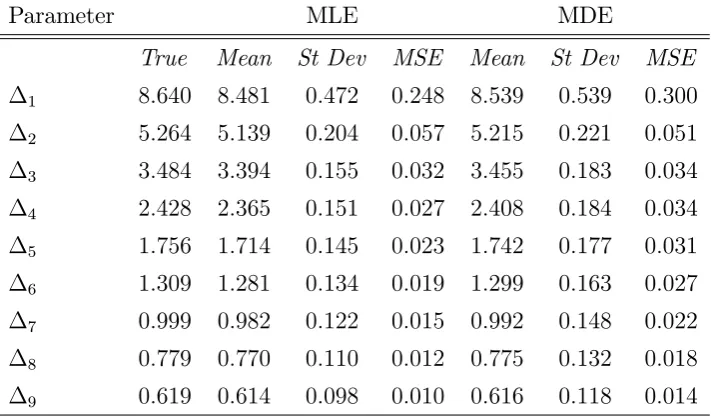
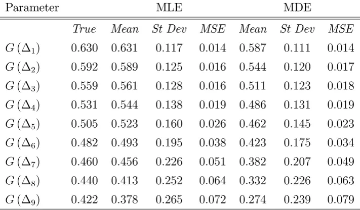
True Mean St Dev MSE Mean St Dev MSE

1 8:640 8:481 0:472 0:248 8:539 0:539 0:300 2 5:264 5:139 0:204 0:057 5:215 0:221 0:051 3 3:484 3:394 0:155 0:032 3:455 0:183 0:034 4 2:428 2:365 0:151 0:027 2:408 0:184 0:034 5 1:756 1:714 0:145 0:023 1:742 0:177 0:031 6 1:309 1:281 0:134 0:019 1:299 0:163 0:027 7 0:999 0:982 0:122 0:015 0:992 0:148 0:022 8 0:779 0:770 0:110 0:012 0:775 0:132 0:018 9 0:619 0:614 0:098 0:010 0:616 0:118 0:014

Table 2: Properties of maximum likelihood (MLE) and minimum distance (MDE) estimators for

Parameter MLE MDE

True Mean St Dev MSE Mean St Dev MSE

G( 1) 0:630 0:631 0:117 0:014 0:587 0:111 0:014 G( 2) 0:592 0:589 0:125 0:016 0:544 0:120 0:017 G( 3) 0:559 0:561 0:128 0:016 0:511 0:123 0:018 G( 4) 0:531 0:544 0:138 0:019 0:486 0:131 0:019 G( 5) 0:505 0:523 0:160 0:026 0:462 0:145 0:023 G( 6) 0:482 0:493 0:195 0:038 0:423 0:175 0:034 G( 7) 0:460 0:456 0:226 0:051 0:382 0:207 0:049 G( 8) 0:440 0:413 0:252 0:064 0:332 0:226 0:063 G( 9) 0:422 0:378 0:265 0:072 0:274 0:239 0:079

Table 3: Properties of maximum likelihood (MLE) and minimum distance (MDE) estimators for

G( 1); : : : ; G( 9).

Tables 1 and 2 contain the true mean and standard deviation of various parameters for each estimator as reported in MGW,11 _{in addition we include the mean square errors for the ease of}

comparison between our results and theirs (that include the empirical likelihood estimator). We provide the same statistics for the estimator of the cdf evaluated at the cuto¤ points in Table 3. Our estimator performs comparably well with respect to the maximum likelihood estimator. Particularly our estimator generally has smaller bias, but also higher variance. However, there is no dominant estimator with respect to the mean square errors, at least for this design and sample size. Our estimator appears to generally perform better for the parameters in Table 1. The maximum likelihood estimation is better for those in Table 2. The results are more mixed for Table 3.

Next we consider the estimation of data that come from several markets. Here we adopt the same design to the one used to generate results in the Supplementary Appendix that accompanies MGSW. The data are drawn from 10 heterogeneous markets. The consumers have the same search cost distribution in every market while sellers’ marginal costs can vary and thus imply di¤erent equilibrium price distribution. For each simulation we draw 35 prices from the equilibrium price distribution from each market. So the total sample size is 350. Other details can be found in MGSW.

that de…ne Bernstein polynomials of order Lconsists of the following L+ 1 functions:

glL(c) =

L!

l! (L l)!c

l_{(1 c)}L l

; l = 0; : : : ; L:

We choose Bernstein polynomials due to its well-behaved uniform property as well as the simplicity to impose shape restrictions one expects from a cdf12_{. See Lorentz (1986) for further details. For a}

generic support, _SC = C; C , we can scale the support of functions in GT accordingly. We impose

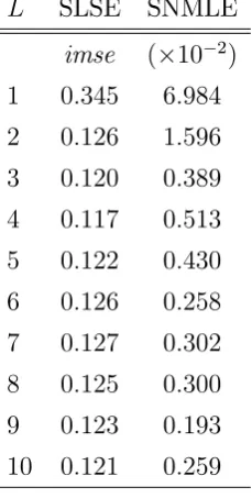
monotonicity in estimating our sieve estimator in the simulation study and the application. For the estimator of MGSW we use Hermite polynomials as the basis as done in their paper. We report in Table 4 the integrated mean square error (imse), de…ned as R EhGb(c) G(c)i

2

dG(c), for our estimator and theirs for the …rst corresponding 10basis terms.

L SLSE SNMLE

imse ( 10 2₎

1 0:345 6:984

2 0:126 1:596

3 0:120 0:389

4 0:117 0:513

5 0:122 0:430

6 0:126 0:258

7 0:127 0:302

8 0:125 0:300

9 0:123 0:193

10 0:121 0:259

Table 4: Imse for sieve least squares (SLSE) and semi-nonparametric maxmimum likelihood (SNMLE) estimators using Lbasis functions.

We note that it would not be appropriate to compare our reported statistics and Table 1 of MGSW. In particular the imse we use is di¤erent to their integrated squared error. There are two

12_{For any continuous function g:}

lim

L!1

L X

l=0 g l

L

L!

l! (L l)!c

l_{(1 c)}L l

=g(c);

holds uniformly on [0;1]. Furthermore for _GT = g:g=gL>b for someb= (b0; : : : ; bL) , elements in GT will be

non-decreasing under the restrictions that bl bl+1 for l= 0; : : : ; L, and the range of functions inGT can be set by

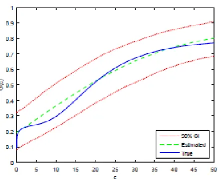
Figure 1: Sieve estimator of the cost cdf with L= 4.

di¤erences. First, their integrated error is calculated by integrating the squared error between the Monte Carlo average of Gb and the true. Second, their integrator is the identity function and ours is

G; i.e. we use R [ ]dG(c) rather than R [ ]dc.

Figure 2: Sieve estimator of the cost cdf with L= 9.

Figure 3: MGSW’s estimator of the cost cdf withL= 4.

5.2

Empirical Illustration

Background and Data

Gambling in the UK is regulated by the Gambling Commission on behalf of the government’s Department for Culture, Media and Sport under the Gambling Act 2005. In addition to the moral duty to prevent the participation of children and the general policing against criminal activities related to gambling in the UK, another main goal of the Act is to ensure that gambling is conducted in a fair and open way. One crucial component of the Act that has received much attention in the media takes place in September 2007, which permits gambling operators to advertise more widely.13

Its intention is to raise the awareness for the general public about potential bookmakers in the market in order to increase the competition between them.

In this section we illustrate the use of our estimators proposed in earlier parts of the paper. We assume the search model described in Section 2 serves as a (very) crude approximation of the true mechanism that generates the prices that we see in the data.14 _{We focus on the booking odds set}

at di¤erent bookmakers for the top two professional football leagues in the UK, namely the Premier League and the League Championship, for the 2006/7 and 2007/8 seasons. We consider the odds for what is known as a “2x1 bet”, where there are three possible outcomes for a given match: home (team) wins, away wins or they draw. We construct the price for each bookmaker from the odds we observe. Since the odd for each event is the inverse of its perceived probability, we de…ne our price from each bookmaker as: 1/(home-win odd) + 1/(draw odd) + 1/(away-win odd). The sum of theses probabilities always exceeds 1 since consumers never get to play a fair game. This excess probability represents what is called the bookmaker’s overround. The higher the overround, the more unfair and expensive is the bookmaker’s price.

We obtain the data from http://www.oddsportal.com/, which is an open website that collects

13_{Gambling operators have been able to advertise on TV and radio from 1st of September 2007.}

Previ-ously the rules for advertising for all types of gambling companies, including casinos and betting shops have been highly regulated. Traditional outlets for advertising are through magazines and newspapers, or other

means to get public attention such as sponsoring major sporting events. Further information on the back-ground and impact of the Gambling Act 2005 can be found in the review produced by the Committees of Ad-vertising Practice at the request by the Department for Culture, Media and Sport,

http://www.cap.org.uk/News-reports/~/media/Files/CAP/Reports%20and%20surveys/CAP%20and%20BCAP%20Gambling%20Review.ashx

14_{We highlight three underlying assumptions of the theoretical model. First, products are homogeneous. Second,}

consumers perform a non-sequential search. Third, each consumer purchases only one unit of the product. In the context of betting it is not unreasonable to assume products are homogeneous as consumers are only interested in making monetary pro…t. Our prices are based on online odds therefore non-sequential search strategy may also provide

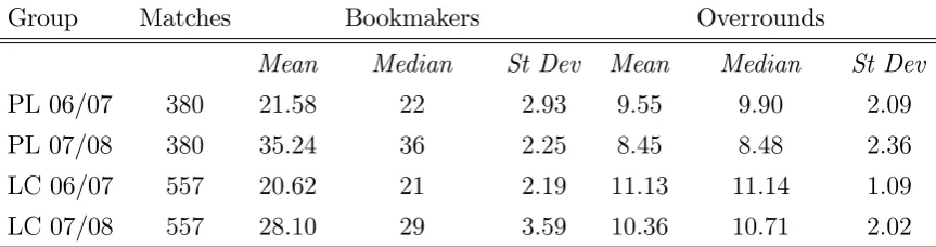
data from the main online bookmakers from a number of di¤erent events. In the tables and …gures below, we use PL and LC to respectively denote Premier League and League Championship, and 06/07 and 07/08 respectively for the 2006/7 and 2007/8 seasons. We begin with Table 5 that gives some summary statistics on the data.

Group Matches Bookmakers Overrounds

Mean Median St Dev Mean Median St Dev

PL 06/07 380 21:58 22 2:93 9:55 9:90 2:09

PL 07/08 380 35:24 36 2:25 8:45 8:48 2:36

LC 06/07 557 20:62 21 2:19 11:13 11:14 1:09

LC 07/08 557 28:10 29 3:59 10:36 10:71 2:02

Table 5: Summary statistics on the data from di¤erent leagues and seasons.

We partition the data into four product groups. One for each league and season. The numbers of bookmakers we observe vary between matches as occasionally odds for some bookmakers have not been collected. The average overrounds between the two seasons indicate that prices have fallen after the change of law. Relatedly, we also see an increase in the average number of bookmakers as well.15 For each group we take the number of sellers to be the average number of bookmakers (rounded to the nearest integer). We treat the observed price for every match as a random draw from an equilibrium price distribution. We assume the distribution of the consumers’search cost to be the same for both leagues within each season. Our main interest is to see if there is any evidence the distribution of the search costs di¤er between the two seasons.

Single Market

We provide four sets of point estimates. One for each group using the estimator described in Section 3. For the following tables, the bootstrap standard errors are reported in parentheses.

Group K q_b1 qb2 qbK r(bq) p p

PL 06/07 23 0:77 0:21 0:01 80:36 100:09 118:99

(0:03) (0:02) (0:00) (2:20)

PL 07/08 36 0:40 0:55 0:05 96:40 100:04 125:62

(0:10) (0:08) (0:00) (1:13)

LC 06/07 22 0:67 0:30 0:03 97:51 105:03 118:04

(0:10) (0:08) (0:00) (4:78)

LC 07/08 29 0:20 0:73 0:07 97:87 101:23 159:30

(0:11) (0:10) (0:01) (0:98)

Table 6: Estimates of search proportions, selling costs and range of prices

Over 90% of consumers search at most twice for every product group. Other proportions of con-sumers’search that are not reported are very close to zero. It is very noticeable that the proportions of consumers searching just once drop, following the law change, transferring mostly to searching twice. We now relate these to the search cost distribution.

Group K b1 Gb( 1) b2 Gb( 2) bK 1 Gb( K 1)

PL 06/07 23 2:49 0:23 1:24 0:01 0:07 0:01

(0:05) (0:02) (0:02) (0:00) (0:00) (0:00)

PL 07/08 36 3:17 0:60 1:26 0:05 0:03 0:05

(0:40) (0:09) (0:10) (0:01) (0:00) (0:01)

LC 06/07 22 1:72 0:33 0:83 0:03 0:05 0:03

(0:08) (0:08) (0:08) (0:01) (0:01) (0:01)

LC 07/08 29 6:07 0:80 1:98 0:07 0:04 0:07

(1:18) (0:12) (0:24) (0:01) (0:00) (0:01)

Table 7: Estimates of search cost distribution

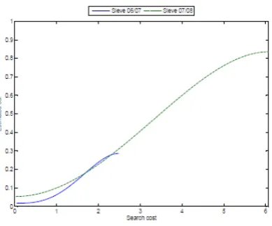
We do not report the estimated cdf values for other cut-o¤ points since they are almost identical toGb( 2)andGb( K 1). Since the cut-o¤ values for each group di¤er, it is more convenient to make

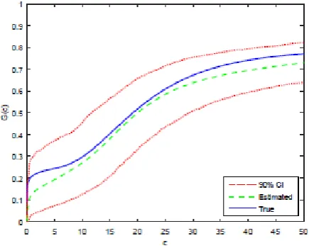
this comparison graphically. We next estimate the cdf as a function.

Pooling Data Across Markets

Figure 5: Scatter plots of the point estimates of cost quantiles for the two football leagues, and the corresponding sieve estimates of the cost cdf using data from the 2006/7 season.

Figure 6: Scatter plots of the point estimates of cost quantiles for the two football leagues, and the corresponding sieve estimates of the cost cdf using data from the 2007/8 season.

see the description above. To construct our estimates for the cdfs we only impose monotonicity on the coe¢ cients to ensure the estimates are non-decreasing. We …t the data using L= 4.

Figure 7: Sieve estimates of the cost cdf using data from the 2006/7 and 2007/8 seasons.

6

Conclusion

Appendix

Preliminary Notations

The proofs of our Theorems make use of some results from empirical processes theory. We do not de…ne basic terms and de…nitions from empirical processes theory here for brevity. We refer the reader to the book by Kosorok (2008) for such details.

Firstly, with an abuse of notation, it will be convenient to introduce a functionm(; ; ) :_SP !R

that depends respectively on …nite and in…nite dimensional parameters ₂ and ₂ . Recall that = [0;1]K 1. Here we use to denote a set of all cdfs with bounded densities de…ned on _SP.

So that for p_{2 S}P, 2 and 2 , we de…ne:

m(p; ; ) = 1 p p K

K_X1

k=1

(k K) k

!!

0

@ K 1

PK 1

k=1 k (1 (p))

K 1

+PK_k=11 k(1 (p))k 1

1

A (p p) 1 p p K

K_X1

k=1

(k K) k

!!

:

Comparing the above to the function m(; ) used in the main text (see e.g. (8)), we have that

m(; ) and m(; ; F) are precisely the same objects.

We denote a space of bounded functions de…ned on _SP equipped with the sup-norm by D. We

view m(; ; ) as an element in_D, which is parameterized by( ; )₂ . Also since is de…ned in m(p; ; ) pointwise for each p, it will be useful in the proofs below for us to occasionally write

m(p; ; (p)) m(p; ; ) in de…ning some derivatives for clarity. In particular, pointwise for each

p, using an ordinary derivative, for any let: D m(p; ; (p)) limt!0 m(p; ; (p)+t)_t m(p; ; (p)) and D _@@

km(p; ; (p)) limt!0 @

@ km(p; ; (p)+t) @

@ km(p; ; (p))

t for all k. It is easy to see that m(; ; ), @

@ km(; ; ), D m(; ; ) and D

@

@ km(; ; ) are elements in D for any ( ; ) in . In the

main text we have denoted the sup-norm for any real value function de…ned on _SC by j j₁. In

this Appendix we will also use _{j j1} to denote the sup-norm for any real value function de…ned on

SP as well. We do not index the norm further to avoid additional notation. There should be no

ambiguity whether the domain for the function under consideration is _SP or SC. We de…ne the

following constants that will be helpful in guiding the reader through our proofs:

m = sup

( ; )2 j

m(; ; ( ))_j1; @

@ m = max_{1 k K} sup

( ; )2

@ @ k

m(; ; ( ))

1

;

DFm = sup

( ; )2 j

DFm(; ; ( ))j₁; _DF @

@ m = max_{1 k K} sup

( ; )2

DF

@ @ k

m(; ; ( ))

1

Other generic positive and …nite constants that do not depend on the sample size are denoted by ₀, which can take di¤erent values in di¤erent places.

Lemmas

Lemmas 1 - 8 are used to prove Theorems 1 - 3 from Section 3. Lemmas 9 - 17 are used to prove Theorem 4 from Section 4.

Lemma 1. Under Assumptions A2(i) and A2(ii), M( ) has a well-separated minimum at 0.

Proof of Lemma 1. Under A2(i) and the domination condition in A2(ii), M has a unique minimum at 0. Since M is continuous on , the minimum is well-separated.

Lemma 2. Under Assumptions A2(i) and A2(ii), sup _{2 j}MN( ) M( )j a:s:

! 0.

Proof of Lemma 2.

MN( ) M( ) =

Z

m(p; ; FN)2( N(dp) (dp)) +

Z

m(p; ; FN)2 m(p; ; F)2d

= I1( ) +I2( ):

For I1( ), using the bound for m, jI1( )j 2m

R

( _N(dp) (dp)). The convergence of measure follows from A2(ii) so that sup _{2 j}I1( )j

a:s:

! 0. For I2( ), we have

jI2( )j 2 m

Z

jm(p; ; FN) m(p; ; F)j (dp)

2 _{m D}

Fm

Z

(dp)_jFN Fj₁:

The second inequality follows from taking pointwise mean value expansion aboutF. Thensup _{2 j}I2( )j

a:s:

!

0 by Glivenko-Cantelli theorem. The proof then follows from the triangle inequality.

Let

H( ) =

Z

2 @

@ m(p; ; F) @

@ >m(p; ; F) (dp);

HN( ) =

Z

2 @

@ m(p; ; FN) @

@ >m(p; ; FN) N(dp);

H_N( ) =

Z

2 @

@ m(p; ; FN) @

@ >m(p; ; FN) N(dp);

where F_N is the empirical cdf with respect to the bootstrap sample.

Lemma 3. Under Assumption A2(ii), for any N such thatk N 0k

a:s:

! 0then_kHN( N) H( 0)k

a:s:

!

Proof of Lemma 3. First show sup _{2 k}HN( ) H( )k a:s:

! 0. Using the same strategy in the proof of Lemma 2, let h(p; ; ) = 2@

@ m(p; ; ) @

@ >m(p; ; ), we have:

HN ( ) H( ) =

Z

h(p; ; FN) N(dp)

Z

h(p; ; F) (dp) =

Z

h(p; ; FN) ( N(dp) (dp)) +

Z

h(p; ; FN) h(p; ; F) (dp)

= J1( ) +J2( ):

Thensup _{2 k}J1( )k 0 2@ @ m

R

( _N (dp) (dp))a:s:_! 0, andsup _{2 k}J2( )k 0 2_DF @ @ m

R

(dp)_jFN Fj₁

a:s:

!

0. Uniform almost sure convergence then follows from the triangle inequality. By the continuity ofH( ) and Slutzky’s theorem,_jH( N) H( 0)j

a:s:

!0.

The desired result holds by using the triangle inequality to bound HN(b) H( 0) = HN(b)

H(b) +H(b) H( ).

Lemma 4. Under Assumption A2(ii), _@@ MN( 0)

d

! N (0; ).

Proof of Lemma 4. From its de…nition, _@@MN( 0) = 2

R @

@ m(p; 0; FN)m(p; 0; FN) N(dp),

by adding nulls we have

p

N @

@ MN( 0)

= 2

Z _@

@ m(p; 0; F)

p

N m(p; 0; FN) (dp) +2

Z

@

@ m(p; 0; FN) @

@ m(p; 0; F)

p

N m(p; 0; FN) (dp) +2

Z _@

@ m(p; 0; F)

p

N m(p; 0; FN) ( N(dp) (dp)) +2

Z

@

@ m(p; 0; FN) @

@ m(p; 0; F)

p

N m(p; 0; FN) ( N(dp) (dp))

= J1+J2 +J3+J4:

We …rst show the desired distribution theory is delivered by J1.

By Donskers’theorem the empirical cdf converges weakly to a standard Brownian bridge of F, denoted by (_B(F (p)))_p2S

P. So that for p; p

0 _{2 S}

P,

B(F (p)) _N(0; F (p) (1 F (p))), and (16)

Cov (_B(F (p));_B(F (p0))) = F (min_fp; p0_g) F (p)F(p0):

In this proof, it will be convenient to de…ne my_{(; ) = m(;}