Simulating sub-daily Intensity-Frequency-Duration curves in Australia using
1
a dynamical high-resolution regional climate model
2 3 4
Gabriel A. Mantegna a ([email protected]) 5
Christopher J. White b, c *([email protected]) 6
Tomas A. Remenyi c ([email protected]) 7
Stuart P. Corney c ([email protected]) 8
Paul Fox-Hughes c, d ([email protected]) 9
10
a Department of Environmental Health and Engineering, Johns Hopkins University, 3400 North
11
Charles Street, Baltimore, Maryland 21218, USA 12
b School of Engineering and ICT, University of Tasmania, Private Bag 65, Hobart, TAS, 7001,
13
Australia 14
c Antarctic Climate and Ecosystems Cooperative Research Centre, Private Bag 80, Hobart,
15
Tasmania, 7001, Australia 16
d Bureau of Meteorology, 5/111 Macquarie St, Hobart, Tasmania, 7000, Australia
17 18 19 20 21 22 23 24
Accepted for publication in Journal of Hydrology 25
26 27
* Corresponding author: 28
Dr Christopher J. White 29
Postal address: School of Engineering and ICT, University of Tasmania, Private Bag 65, Hobart, 30
TAS, 7001, Australia 31
Telephone number: +61 (0) 3 6226 7640 32
Email address: [email protected] 33
Abstract
35
Climate change has the potential to significantly alter the characteristics of high-intensity, short-36
duration rainfall events, potentially leading to more severe and more frequent flash floods. 37
Research has shown that future changes to such events could far exceed expectations based on 38
temperature scaling and basic physical principles alone, but that computationally expensive 39
convection-permitting models are required to accurately simulate sub-daily extreme rainfall 40
events. It is therefore crucial to be able to model future changes to sub-daily duration extreme 41
rainfall events as cost effectively as possible, especially in Australia where such information is 42
scarce. In this study, we seek to determine what the shortest duration of extreme rainfall is that 43
can be simulated by a less computationally expensive convection-parametrizing Regional 44
Climate Model (RCM). We examine the ability of the Conformal Cubic Atmospheric Model 45
(CCAM), a ~10 km high-resolution convection-parametrizing RCM, to reproduce sub-daily 46
Intensity-Frequency-Duration (IFD) curves corresponding to two long-term observational 47
stations in the Australian island state of Tasmania, and examine the future model projections. We 48
find that CCAM simulates observed extreme rainfall statistics well for 3-hour durations and 49
longer, challenging the current understanding that convection-permitting models are needed to 50
accurately model sub-daily extreme rainfall events. Further, future projections from CCAM for 51
the end of this Century show that extreme sub-daily rainfall intensities could increase by more 52
than 15 % per °C, far exceeding the 7 % scaling estimate predicted by the Clausius-Clapeyron 53
vapour pressure relationship and the 5 % scaling estimate recommended by the Australian 54
Keywords 56
sub-daily rainfall; extremes; Intensity-Frequency-Duration; Depth-Duration-Frequency; flood; 57
1. Introduction
59
Heavy rainfall events with durations of less than 24 hours are a triggering factor for many high-60
impact natural hazards, including flash floods, landslides and debris flows. These hazards pose 61
significant risk to people, infrastructure and systems. Climate change has the potential to alter 62
both the prevalence and severity of rainfall extremes and floods (Bates et al., 2016), with 63
intensification of heavy rainfall events becoming evident in the observed record across many 64
regions of the world (Fischer and Knutti, 2016), necessitating an improved understanding of how 65
they may change in the future. 66
67
Dynamical Regional Climate Models (RCMs) have been used to produce estimates of the future 68
changes to more extreme, multi-day rainfall events across Australia (e.g. White et al., 2013; 69
Perkins et al., 2014; Evans et al., 2016; Li et al., 2016; 2017). There exists, however, 70
considerable uncertainty in future extreme rainfall projections, particularly for the sub-daily 71
intensities (Johnson et al., 2016). To date, few studies have examined sub-daily rainfall extremes 72
in Australia. This paucity of studies is due to a combination of sparse observations, the inability 73
of broad-scale Global Climate Models (GCMs) to reliably simulate sub-daily rainfall (Chan et 74
al., 2014b), and the costs associated with high-resolution climate modelling. Variations in 75
frequency and magnitude of observed events at daily durations have also been found to be a poor 76
indicator of changes at sub-daily durations (Jakob et al., 2011); as such, multi-day rainfall 77
projections cannot be directly used to inform changes in sub-daily-duration rainfall. Yet it is 78
these short duration rainfall intensities that are of particular interest to practitioners and decision-79
82
While recent progress has been made towards understanding and modelling hourly rainfall 83
intensities internationally (notably Lenderink and van Meijgaard (2008) for the Netherlands, 84
Kendon et al. (2012) and Chan et al. (2014a; 2014b; 2016) for the UK, and Sunyer et al. (2017) 85
for Denmark), there is a paucity of both sub-daily rainfall observations and climate change 86
projections across Australia. Although there is an extensive record of daily rainfall observations 87
available from the Bureau of Meteorology (BoM), spanning several decades – and in some cases, 88
over 100 years in length – high-quality sub-daily (e.g. 6-min continuous) rainfall observations 89
from pluviographs or Tipping Bucket Rain Gauges are far more limited, with such data often 90
much shorter in length (typically with a record of less than 25 years). To adequately sample the 91
effects of climate variability on rainfall extremes long, homogeneous time series are required 92
(Jakob et al., 2011). Due to these limitations there have been few studies of these continuous 93
sub-daily observations to date (see Jakob et al. (2011) and Zheng et al. (2015) for studies of 94
trends in sub-daily rainfall durations in the Sydney region, where sub-daily rainfall trends are 95
found to differ from multi-day trends). Because of the limited spatial availability of sub-daily 96
observations, no gridded sub-daily rainfall product exists for Australia, making the evaluation of 97
modelled sub-daily rainfall extremes a significant challenge (Rummukainen et al., 2015). 98
99
The Australian Rainfall and Runoff (ARR) (Ball et al., 2016) is the main guide used by 100
Australian engineers and hydrologists to combine statistical methods and observations to 101
estimate return levels and design rainfalls. The 2016 revision of ARR includes new Intensity-102
2015; Bureau of Meteorology, 2016)1. These curves were generated using a quality-controlled 104
homogenised database comprising rainfall data from the BoM's rain gauge network and data 105
from rainfall recording networks operated by other organisations (Green et al., 2012; 2016). In 106
the absence of spatially and temporally consistent sub-daily and multi-day future rainfall 107
projections, interim guidance has been provided to allow for a range of plausible future changes 108
to rainfall to be applied to the IFD curves (Bates et al., 2016). Uncertainty in broad-scale GCM 109
rainfall projections is, however, generally high; Bates et al. (2016) suggest using 5 % as the 110
default percentage change in heavy rainfalls per °C of warming but note that this could in reality 111
be between 2 % and 15 % per °C of warming. As such the ARR approach uses a simple 112
adjustment factor of 5 % per °C of warming, based on projected temperature increases from a 113
consensus of GCM simulations for a given future realisation (or ‘class interval’) of ‘slightly 114
warmer’ (< 0.5 °C), ‘warmer’ (0.5 to 1.5 °C), ‘hotter’ (1.5 to 3 °C) or ‘much hotter’ (> 3 °C). 115
This method applies a corresponding regional correctional value to the IFDs producing a 116
projected increase in rainfall intensity. 117
118
This method used in ARR is based on the understanding that daily rainfall increases with 119
temperature at a rate of approximately 7 % per °C according to the Clausius-Clapeyron water-120
holding capacity relationship between temperature and vapour pressure (Trenberth et al., 2003). 121
In contrast to daily cumulative rainfall it has been found that daily and sub-daily heavy rainfall 122
intensities do not consistently follow the Clausius-Clapeyron relationship due to the additional 123
latent heat released from increased atmospheric moisture (Lenderink and van Meijgaard, 2008; 124
1It should be noted that the name for Intensity-Frequency-Duration curves varies by country. In
Depth-Duration-Liu et al., 2009). Depth-Duration-Liu et al. (2009) found that global average daily rainfall intensity increases by 125
about 23 % per °C, significantly exceeding the ~7 % per °C from the Clausius-Clapeyron 126
relationship. At the sub-daily timescale, Lenderink and van Meijgaard (2008) found that the 127
observed intensity of hourly rainfall extremes at a station in the Netherlands increases twice as 128
fast per °C as expected from the Clausius-Clapeyron relationship when daily mean temperatures 129
exceed 12 °C. This observed trend was matched in the same study by simulations using a high-130
resolution regional climate model showing that one-hour extreme rainfall intensities increase at a 131
rate close to 14 % per °C of warming across large parts of Europe. By using medium- and high-132
resolution RCMs, Chan et al. (2014a) similarly found that future extreme hourly rainfall 133
intensities in the southern UK cannot simply be extrapolated using a present-climate temperature 134
scaling approach. 135
136
Dynamical climate models need to be of sufficient resolution to capture the large-scale 137
influences of various climate modes, the diurnal and seasonal cycles, and the regional and local 138
scale convection-permitting and orographic wind processes that are the proximate cause of 139
extreme rainfall (Westra et al., 2014; Rummukainen et al., 2015; Cortés-Hernández et al., 2016; 140
Johnson et al., 2016; Kendon et al., 2017). Lower-resolution dynamical models, for example, 141
have been shown to contain large rainfall biases (Kjellström et al., 2010), poor timing and 142
durations (Brockhaus et al., 2008), and inaccurate spatial distributions (Gregersen et al., 2013). 143
Spatial model resolution also influences the quality of the representation of dynamical rainfall 144
projection, especially for extremes over short timescales that are more likely to be dominated by 145
convection (Chan et al., 2014b; Sunyer et al., 2017). Although statistical downscaling methods 146
dynamical climate models that can likely simulate this temperature-rainfall relationship (Ban et 148
al., 2014). 149
150
High-resolution (~10 km grid) dynamically downscaled climate change simulations have been 151
produced for Australia’s island state of Tasmania using a convection-parametrizing RCM by the 152
Climate Futures for Tasmania project (Corney et al., 2010; 2013). These simulations – the most 153
recent high-resolution regional climate projections for Tasmania – have been extensively 154
analysed for a range of extremes including rainfall, projecting increases in maximum 1- and 5-155
day rainfall intensities separated by longer dry spells (White et al., 2010; 2013). Projections for 156
Hobart and Launceston – the two most populous areas of the state – suggest that the 1 % Annual 157
Exceedance Probability (AEP) intensity for 24-hour duration rainfall totals will increase by about 158
25 % in both locations by the end of the Century (White et al., 2010). These previous studies, 159
however, primarily rely on daily rainfall values. As a consequence, we therefore have limited 160
understanding of how the projected changes in daily rainfall across Tasmania translate to sub-161
daily intensities. 162
163
As part of the Climate Futures for Tasmania project, a multi-model high-resolution 6-minute 164
dataset was produced at 14 discrete locations across Tasmania, corresponding approximately to 165
the high-quality BoM network stations distributed across the state. In this study, we use these 166
continuous 6-minute simulations for the first time to generate IFDs at the main population 167
centres of Hobart and Launceston. The objective of this study is to test how an RCM simulates a 168
range of sub-daily design rainfall intensities compared to observed values covering the 169
allowance for climate change recommended in the ARR 2016 interim guide is appropriate for all 171
rainfall durations and intensities. We seek to find the shortest duration of extreme rainfall events 172
that is accurately simulated by our convection-parametrizing RCM, in order to find the limit of 173
applicability of these types of models. 174
175
This paper is outlined as follows: section 2 details the models, observations, and analytical 176
methods used in this study, section 3 examines the models’ ability to reproduce observed 177
extreme rainfall statistics, section 4 examines the models’ projections for the future, and section 178
5 provides a discussion. 179
2. Materials and methods
180
2.1 Study area
181
Tasmania, an island state southeast of the Australian continental landmass, sits within the 182
westerly wind belt of the Southern Hemisphere. Launceston Airport and Hobart were selected as 183
study locations in Tasmania as they represent the two most populous areas of the state and both 184
have long-term pluviograph records. Both sites are at least somewhat sheltered from the 185
prevailing westerlies by the orography of the western half of Tasmania. Hobart lies at the mouth 186
of the Derwent River in southeast Tasmania, experiencing a mean rainfall of approximately 50 187
mm per month. For most of the year, rainfalls are due to the passage of cold fronts in the 188
westerly airstream. Hobart’s highest daily rainfalls, however, tend to occur during occasional 189
east to southeasterlies associated with extratropical cyclones, where upwards of 50 mm can fall 190
the valley defined by the Tasmanian Central Plateau to the west and northeast highlands to the 192
east. Monthly rainfall for Launceston Airport ranges from 40 mm in late summer to 80 mm in 193
winter. This site is more exposed to moist northwesterly airstreams associated with broad troughs 194
and, particularly, the cold frontal systems often embedded in such troughs. These unstable 195
northwesterly airstreams provide Launceston Airport with its highest daily rainfalls, and many of 196
its most intense sub-daily rainfall totals. Remaining sub-daily intense rainfalls do occasionally 197
occur in weakly forced synoptic situations, generally during the warm season in slow-moving 198
thunderstorms. 199
200
This study has two parts: a comparison between observed data and modelled data for 1961-2009; 201
and a comparison between modelled data for 1961-2009 with modelled data for 2070-2099. We 202
first examine the annual maximum (AMAX) timeseries for each of the two comparisons, and 203
then use this AMAX data to examine the IFD relationships for each comparison. Tasmania, like 204
much of south-east Australia, has experienced a decrease in rainfall since 1975 (Gallant et al., 205
2007). Across Tasmania there was no statistically significant trend in mean annual rainfall 206
between 1910 and 1990 (Srikanthan and Stewart, 1991); however, there has been a downward 207
trend in rainfall between 1970 and 1995 (Shephered, 1995). Across south-east Australia there has 208
been a slight downward trend in rainfall between 1910 and 2005 (Gallant et al., 2007). Future 209
projections of rainfall for Tasmania indicate a change in mean annual rainfall of less than 100 210
mm between 1961 and 2100 (Grose et al., 2010), although note that this result conceals more 211
significant changes at seasonal and regional scales (Grose et al., 2013). We use 1961-2009 as the 212
using this longer time period we maximise the number of observational data points used in the 214
analysis, thus reducing the opportunity for bias. 215
2.2 Observed data
216
The observed rainfall data for this study were recorded using Tipping Bucket Rain Gauges 217
(TBRG) at two locations, Hobart Ellerslie Road (station number 94029) and Launceston Airport 218
(station number 91104). These datasets are in the form of six-minute rainfall totals, collected 219
using digitized pluviograph records from a Dines Tilting Siphon Rain Gauge, and obtained from 220
the Bureau of Meteorology (BoM). 221
222
Both sites contain a large amount of missing data. For Hobart, 58 % of the observed data is 223
missing, and for Launceston, 65 % of the observed data is missing (in both locations, for the 224
1961-2009 time period examined in this study). The distribution of the missing data is assumed 225
to be random, as it occurred due to missing and/or degraded paper pluviograph records without 226
any particular temporal pattern. There are no significant gaps in the timeseries; rather, missing 227
data occurs randomly throughout the entire time period. 228
229
The observed data is put through a two-step quality control process to minimize any erroneous 230
observations. First, any individual six-minute observations with greater than 20 mm of rainfall 231
are ignored. While observations of greater intensity have occurred globally, this is above the 232
range reliably observed in Tasmania. Second, the total of all six-minute observations over each 233
day is compared to the corresponding 24-hour datum, which was recorded with a different 234
corresponding 24-hour observation by more than 20 % and simultaneously by at least 5 mm, the 236
observations from the entire day are ignored. In summary, for Hobart, the observed data we start 237
with for 1961-2009 has 1,802,191 valid observations (not counting missing data), and after 238
quality control we end up with 1,800,030 observations that we use in the study. For Launceston, 239
we start with 1,493,457 valid observations, and after quality control we end up with 1,489,617 240
observations that we use in the study. 241
2.3 Modelled data
242
The modelled data for this study is obtained from the Climate Futures for Tasmania project. The 243
methods are described in full in Corney et al. (2010), and are summarized here. 244
245
The Climate Futures for Tasmania project used the Conformal Cubic Atmospheric Model 246
(CCAM) from Australia’s CSIRO research organisation (McGregor and Dix, 2001; McGregor, 247
2005; McGregor and Dix, 2008). CCAM is a global atmospheric model that uses a stretched 248
cubic conformal grid utilising the Schmidt transformation (1977) with higher resolution in areas 249
of interest (Tasmania). The grid has a resolution of ~10 km per grid cell over the primary face 250
(covering Tasmania) with variably lower resolution over the remainder of the globe. As CCAM 251
is an atmospheric RCM, it is forced by sea surface temperature (SST) as the bottom boundary 252
condition. CCAM uses a semi-Lagrangian advection scheme and semi-implicit time integration 253
with an extensive set of physical parameterizations in a hydrostatic formulation. The GFDL 254
parameterizations for long-wave and short-wave radiation (Lacis and Hansen, 1974; 255
Schwarzkopf and Fels, 1991) were used, with interactive cloud distributions determined by the 256
boundary layer scheme based on Monin-Obukhov similarity theory (McGregor et al., 1993). 258
CCAM’s cumulus convection scheme with both downdrafts and detrainment, as well as mass-259
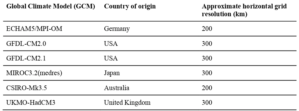
flux closure, is described by McGregor (2003). Six different GCMs were used to force CCAM to 260
produce the model output used for this study, as described in Table 1. 261
262
The dataset used for the current study is the timeseries of rainfall data from CCAM for the SRES 263
A2 high emissions scenario (Nakićenović et al., 2000), with a temporal resolution of 6 minutes. 264
Only data from two grid points is used: the grid point closest to the Hobart Ellerslie Road 265
meteorological station and the grid point closest to the Launceston Airport meteorological station 266
(described above). It should be noted that the elevation of these grid points in the CCAM model 267
is the average elevation over their respective 10 km grid squares, which is different from the 268
actual elevation of the meteorological stations. For the Hobart station, the elevation of the 269
modelled grid point is approximately 150 m higher than the actual elevation of the station, since 270
this grid square contains the lower slopes of Mount Wellington (elevation 1271 m). For the 271
Launceston station, the elevation of the modelled grid point and the elevation of the station are 272
approximately the same, as the landscape is fairly flat near this station. These two locations, 273
Hobart and Launceston Airport, are chosen because they have the most complete observed 274
datasets. 275
2.4 IFD curves
276
After the timeseries of 6-minute rainfall totals is obtained for each dataset and for each location 277
(observed 1961-2009, modelled 1961-2009, and modelled 2070-2099), the rainfall totals over 278
totals for each duration are found using a method of rolling sums, such that for each 6-minute 280
observation, the total rainfall over the past x hours is found, where x is the duration of rainfall 281
being examined. Thus, the dataset of rainfall totals for each duration (e.g. 1-hour totals) is the 282
same length as the original six-minute dataset. Frequency distribution plots, shown in the 283
Appendix (Fig. A.1 and A.2), serve as the most basic representation of the results. To create 284
these frequency distribution plots, the rolling sum data for each dataset is collected into 150 285
evenly spaced bins, selected based on the minimum and maximum values of the data. 286
287
To create the IFD curves, the timeseries of annual maximum rainfall values (AMAX) is found 288
for each dataset and these are fitted to a Generalized Extreme Value (GEV) distribution. A 289
sample of these fits (3- and 6-hour durations) is shown in the Appendix (Fig. A.3 to A.6). For 290
each of six annual exceedance probabilities (AEPs 1, 2, 5, 10, 20, and 50 %), the corresponding 291
intensity is found using the fitted GEV distribution. This calculation is repeated for each rainfall 292
duration (i.e. 0.5-hour, 1-hour, etc.) and the intensities are plotted. Finally, for each of the six 293
modelled IFD curves, the multi-model mean intensity value is used, with the multi-model min 294
and max values used to estimate the spread of plausible futures presented by the different GCMs. 295
2.5 Assessing modelled IFD curves
296
The ARR guidelines are the Australian industry standard methods for flood estimation. These 297
guidelines were last updated in 2016 (see Ball et al., 2016) and have a recommended approach to 298
incorporate the influence of climate change on flood estimates. ARR suggests an implementation 299
of the Clausius-Clapeyron relation, applying a simple temperature-based scaling to existing flood 300
302
𝐼" = 𝐼%&& × (1 +,--++)/0 (1)
303 304
where: Ip = projected rainfall intensity (e.g. 10 mm/hour); IARR = historical rainfall intensity (e.g. 305
10 mm/hour); CC = magnitude of the Clausius-Clapeyron relation expressed as a percentage 306
(default value is 5 %/°C); and Tm = projected mean temperature change. 307
308
This method is used in this study to rescale the modelled current climate IFDs to compare against 309
the modelled future climate IFDs. The CC values used as inputs for our analyses are 5 % (the 310
default recommended by ARR) and 15 % (the maximum value in the recommended range 311
provided by ARR). The Tm is set to 2.9 °C, corresponding to the mean projected temperature rise 312
reported by Grose et al. (2010) for Tasmania for the end of the Century. 313
3. Evaluation of model performance
314
3.1 Comparison of AMAX timeseries
315
The frequency distributions of AMAX values for the investigated design rainfall durations (0.5, 316
1, 3, 6, 12 and 24 hours) for both observations and simulated data are qualitatively compared 317
(Fig. 1 and 2). There is generally good agreement in both locations for all durations of 3 hours 318
and longer, with similar shape and magnitude of the frequency distributions. There is significant 319
inter-model variability, explained by the differing boundary conditions of each parent GCM. For 320
both locations, for all durations of 3 hours and longer, the observed data is mostly within the 321
323
The only exception to this statement is the 24-hour totals for Launceston, which CCAM tends to 324
overestimate by a noticeable margin. This is also true to a lesser extent for the 6- and 12-hour 325
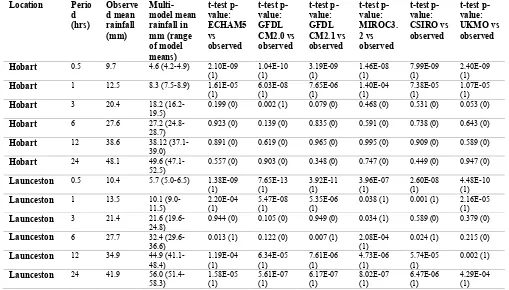
totals (see Table 2). The mean modelled AMAX 24-hour total, averaged across all the models, is 326
56 mm with a range of 51.4 mm to 58.3 mm, whereas the mean observed AMAX 24-hour total is 327
41.9 mm. In contrast, for Hobart the simulations follow the observations well for 3-hour through 328
to 24-hour totals, with a peak in the simulated distributions that align well with those observed 329
(Table 2 and Fig. 1). 330
331
For all durations below 3 hours, the simulations show a higher percentage difference from 332
observed values. CCAM underestimates the AMAX rainfall for the 0.5-hour and 1-hour totals 333
for both locations, with all models displaying a peak at very light rainfall intensities for these 334
times, and not representing any of the heavier falls (such as >10 mm/0.5 hr or >20 mm/hr). 335
Notably, where the six simulations do not agree with observed values, they do agree with each 336
other, indicating that rather than the boundary conditions provided by the parent GCMs driving 337
this difference, it is more likely to be the limitation of the model resolution and how some 338
aspects of rainfall are parameterised, rather than dynamically resolved, within CCAM. 339
3.2 Comparison of IFD curves
340
The IFD curve comparisons (Fig. 3 and 4) support the conclusion that the CCAM model has 341
greater skill for Hobart than it does for Launceston. For Hobart, the modelled IFD values are 342
mostly within 15 % of the observations for the 3- to 12-hour durations (Table 3). Higher 343
especially for 24-hour durations. For the 0.5- and 1-hour durations, the model output 345
underestimates the intensity compared to the observations, with all modelled values differing 346
from observations by more than 30 %. 347
348
For Launceston, the 3- and 6-hour duration totals are mostly within 15 % of observations (Table 349
3). For shorter durations (0.5- and 1-hour duration totals) the model underestimates intensity by 350
>20 % (up to 50 %). For the longer durations (12- and 24-hour) the model output is consistently 351
higher than the observations by more than 25 % (up to 50 %). For both locations, the modelled 352
IFD values tend to agree better with the observed values for the more frequent events (i.e. higher 353
AEPs) as one may expect. This is consistent with the frequency distributions (Fig. 1 and 2) that 354
show better agreement at low to medium rainfall intensities (thus, more common events) 355
compared to the extreme rainfall totals (uncommon events). 356
357
Based on the comparisons between observed and modelled AMAX histograms and IFD curves, 358
we conclude that the CCAM model output is consistent with the observations (within 15%) for 359
the current climate at the study locations, supporting the argument that the sub-daily CCAM 360
model output is indicative of the climate in Launceston and Hobart for extreme rainfall durations 361
>3 hours. In Launceston the highest consistency occurs for 3- and 6-hour duration events with 362
AEPs greater than 10 %. In Hobart, there is broader confidence, with model output consistent 363
with observations for 3- to 12-hour durations for all AEPs, and 24-hour AEPs greater than 5%. 364
CCAM, however, underestimates the intensity for the shorter-duration events (0.5- and 1-hour) 365
hour), especially in Launceston (consistent with previous work with the 24-hour totals, such as 367
Corney et al. (2010)). 368
4. Future climate projections
369
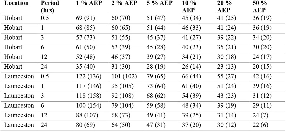
The multi-model assessment generally indicates an increase in rainfall intensity in the future 370
climate at Hobart. The increases in intensity are generally found to be far greater than the default 371
5 % increase per °C recommended for use by industry in ARR (Table 4 and Fig. 5 and 6). The 372
projected increases are non-linear, with largest increases in short-duration, low frequency AEPs 373
and the lowest increases in the long duration high frequency AEPs. This suggests changes are 374
less likely to be driven by the Clausius-Clapeyron relationship, and far more likely to be driven 375
by climatic changes in the prevailing, rain-carrying synoptic systems in the future (Grose et al., 376
2012; Grose et al., 2013). This is supported by the multi-model variability, as the models 377
generally agree on the magnitude of climate warming (Corney et al., 2010), but have different 378
representations of the dominant synoptic features. In both locations, there is significant inter-379
model variability, with MIROC3.2(medres) consistently projecting minimal change into the 380
future, while UKMO-HadCM3 projects large increases in rainfall intensity (up to 200 % in some 381
of the lower AEP classes). This large variability in projected rainfall intensity across the different 382
GCMs is the product of emergent features of the models such as differing mean position of the 383
subtropical ridge, driving different dominant synoptic patterns across the state in the different 384
models (Bennett et al., 2014). This model spread shown in Fig. 5 and 6 indicates that it is these 385
changes in the dynamic processes into the future, resulting in heavier rainfalls, that are more 386
The different dominant synoptic patterns within each model also influence the point-based 389
assessment used in this study, as the distribution and mean rainfall of the target grid cell is 390
affected. Further, Hobart and Launceston are in different climatic regions of Tasmania, and will 391
be influenced by any change in the subtropical ridge in different ways, which is discussed 392
separately below. 393
394
While Hobart receives a high proportion of its rainfall from persistent westerlies, a significant 395
fraction of its annual rainfall occurs in episodic, higher-intensity easterly systems (Fox-Hughes 396
and White, 2015). These systems are by their nature more variable and less predictable than the 397
prevailing westerly conditions. The multi-model spread (see Fig. 5) reflects the range of 398
plausible futures and suggests there is some uncertainty in the exact magnitude of response. 399
CCAM projects 40 to 60 % increases in the intensity of short duration events, and 20 to 30 % 400
increases in longer duration events (Table 4) based on a 2.9 °C temperature change. The 401
magnitudes of these changes are closer to a 15 % increase per °C for short duration events, far 402
exceeding the 5 % default increase per °C recommended by ARR. Additionally, there is 403
significant overlap between historical and future model output, decreasing the certainty of 404
significant changes in the future. 405
406
In contrast to Hobart, Launceston has almost no overlap between the current climate model 407
simulations and the future model projections, indicating a far more distinct increase in rainfall 408
intensities around Launceston. Launceston receives rainfall from both northwesterly and 409
northeasterly systems. As Launceston is further north than Hobart, any change in the position of 410
projects 40 to 120 % increases in the intensity of short-duration events, and 20 to 80 % increases 412
in longer-duration events (Table 4). These greatly exceed the 5 % increase per °C recommended 413
by ARR (Fig. 6), although the largest increases carry with them very low confidence. Focusing 414
on just the durations and AEPs for which we have reasonable confidence (3- to 6-hour AEPs >10 415
%), the projected increases are more reasonable, ranging from 20 to 50 %. 416
417
The future rainfall intensities show an especially significant increase from current conditions for 418
Launceston. Here, the CC temperature scaling estimates are under predictions even for the 24-419
hour duration and especially for the less frequent (lower AEP) events. For example, our average 420
modelled results indicate that the 1 % AEP 3-hour design rainfall event for Launceston could 421
become twice as intense in the future climate (top left plot of Fig. 6). Although there exists 422
significant spread among models for this projection, not one model projects that the increase in 423
intensity will be lower than that estimated by 5 % scaling. 424
425
In short, our results highlight two main patterns in the divergence between the observed and 426
modelled IFD curves: (1) the temperature scaling projections based on 5 % scaling (purple dotted 427
lines) align well with the modelled projections for the highest AEPs and for the 24-hour duration, 428
and (2) the scaling estimates then diverge from the modelled projections for the shorter-duration 429
and less frequent events. There is significant multi-model spread for Launceston, but the 430
modelled results show almost universally that the future rainfall intensities will be higher than 431
5.
Discussion and conclusions
433
In this study, we describe the skill of the CCAM regional climate model in reproducing sub-daily 434
rainfall extremes for Tasmania, and examine projections for future sub-daily values. CCAM is a 435
convection-parametrizing rather than convection-permitting model, and therefore we did not 436
expect the results regarding very short durations (i.e. <1-hour) to be simulated with much skill. 437
Thus, the central aim of this study was to answer the following question: what is the shortest 438
duration at which a convection-parametrizing RCM produces plausible extreme rainfall IFDs? 439
440
At our two test locations of Hobart and Launceston in Tasmania, Australia, we find that CCAM 441
accurately simulates sub-daily extreme rainfall events with durations down to around 3 hours 442
when compared with long-term observations. This result is notable given that CCAM is not a 443
convection-parametrizing model and that a bias-correction was not performed on the data for this 444
study, whereas bias-correction has previously been required for accurate results at longer 24-445
hour durations (e.g. Bennett et al., 2014; Li et al., 2017). These results run counter to previous 446
studies that suggest that very high-resolution convection-permitting models are needed to 447
accurately reproduce sub-daily extreme rainfall events (e.g. Chan et al., 2014b; Westra et al., 448
2014; Johnson et al., 2016; Kendon et al., 2017). We are not suggesting that this previous work is 449
incorrect; rather, we are providing evidence that in some cases, extreme rainfall statistics can be 450
accurately reproduced without using a computationally expensive convection-permitting model. 451
452
The results of this study suggest that model skill likely occurs because the extreme rainfall 453
experienced in the study locations, while often convective in nature, occurs as part of larger 454
CCAM (Corney et al., 2010), which means the relative skill of CCAM may be partially location-456
specific. The differences between modelled and observed values for shorter (i.e. < 3-hour) 457
durations therefore occur because these shorter-period extremes are the result of convective 458
behaviour within larger systems that are not well modelled by CCAM’s ~10 km grid. It is 459
generally assumed that a 1 km or smaller grid scale is needed to use a convection-permitting 460
scheme (Westra et al., 2014). 461
462
Another reason for the model skill is that CCAM is a dynamically downscaled model rather than 463
relying on a statistical scheme to generate local-scale weather phenomena. Several studies have 464
compared the results of statistical and dynamical downscaling, showing that the two methods 465
perform similarly for current climate, but dynamically downscaled models have been shown to 466
be more accurate at producing regional climate change signals (Cubasch et al., 1996; Corney et 467
al., 2013). Dynamical downscaling allows for changes in the local climate, such as changes to 468
seasonality, changes to the frequency and intensity of weather events and the relationships 469
between different climate variables. This behaviour is essential for modelling changes to sub-470
daily extreme rainfall totals. 471
472
One area where our results are somewhat counterintuitive is that CCAM reproduces trends that 473
are closer to observations for Hobart than for Launceston. One would expect the Launceston 474
results to be more reliable as Launceston is relatively flat and far from the ocean, whereas Hobart 475
is a port city on the flank of a mountain. The reason for the increased skill in Hobart could lie in 476
the type of rain-producing weather systems seen in this region. Extreme rainfall events in and 477
by CCAM (Grose et al., 2012). As for Launceston, the lower skill has also been identified by 479
Corney et al. (2010) and Bennett et al. (2014), which show that CCAM over-predicts rain 480
(relative to observations) by as much as 50 % in this region. These studies bias-corrected the 481
daily rainfall to account for this anomaly. As the current study uses uncorrected model output, 482
this difference at the 24-hour duration level was expected. These previous studies also provide 483
possible reasons for the rainfall overestimation for Launceston, the dominant one being 484
Launceston’s proximity to multiple mountain ranges. Due to the topography data resolution, the 485
mountains CCAM interacts with are not nearly as steep and high as the actual mountains, so 486
CCAM underestimates the orographic rainfall that occurs in these mountains. The orographic 487
rainfall in the real world depletes atmospheric moisture before storms pass over Launceston, 488
whereas in CCAM, less upstream orographic rainfall occurs. Crucially these studies showed that 489
the reason for this error was systematic and thus should be consistent into the future. 490
491
A bias-correction (e.g. following Bennett et al., 2014) could be considered to correct for 492
differences between model output and observations. However, bias-correction at the sub-daily 493
level is problematic due to a lack of gridded sub-daily observations against which the model can 494
be compared. Bias-correction at the sub-daily scale can only be undertaken at sites where 495
observations are available therefore (such as the two sites chosen for this study). This is 496
effectively just scaling the distribution of the model output to match observations over the 497
observational period and assuming this scaling remains consistent into the future. For the current 498
study, we eliminate the need for bias-correction by reporting upon relative changes within the 499
model output when we examine future projections. These changes would be the same even with 500
directly used by practitioners; rather, we intend for our study to be a starting point for other 502
studies investigating sub-daily rainfall changes. The key result of our study is the percentage 503
changes in the future projections, not the absolute intensities, which we acknowledge are likely 504
biased in the model. For any future studies that wish to arrive at estimated future rainfall 505
statistics across a wide geographical area for direct use by practitioners, bias-correction of model 506
output will most likely be necessary. 507
508
Our findings regarding the projection of future sub-daily extreme rainfall IFDs add to the 509
existing body of research, showing that extreme rainfall events could intensify much more than 510
the simple Clausius-Clapeyron temperature scaling alone predicts, although these findings 511
should be taken within the context of how well the RCM performed against observations at the 512
study locations (Fig. 3 and 4). Existing studies (e.g. Lenderink and van Meijgaard, 2008; Liu et 513
al., 2009) highlight the additional latent heat released from increased atmospheric moisture as a 514
possible key reason for this behaviour. Further, our results confirm that this exaggerated change 515
could be seen mainly in the less frequent, shorter duration events, which has implications for 516
urban applications where short duration extreme events can cause damaging flash floods. Related 517
to this, another important finding is the confirmation that projected increases for daily extreme 518
events cannot be simply extrapolated to sub-daily durations. The CCAM data show that the 1 % 519
AEP 24-hour events will become about 25 % more intense in the future time period examined 520
(White et al., 2010), whereas the sub-daily data used in this study show that the 1 % AEP 3-hour 521
events could become 100 % more intense, if not more (Fig. 5 and 6). This is a conclusion that 522
has been reached by similar studies (e.g. Lenderink and van Meijgaard, 2008). 523
While our results are promising, they should however be interpreted with some caution. This 525
study focuses on the intensity and frequency of extreme rainfall events, rather than on how 526
accurately these events are simulated from a meteorological processes standpoint. Investigations 527
into the seasonality and meteorological realism of these extreme events could aid model 528
performance and remain an important area for future work. This study is also to some degree 529
location-specific. We suggest that future work should examine whether a regional climate model 530
can produce similarly accurate results for other locations around the world. 531
532
In conclusion, while this study may be limited due to the inherent convection-parametrizing 533
nature of the CCAM model used, in many ways this study is an important pedagogic endeavour. 534
We have sought to find the limit of applicability for convection-parametrizing models, and we 535
believe we have found this approximate limit. Our results show that for areas where extreme sub-536
daily rainfalls do not come principally from convective systems, a convection-parametrizing 537
regional climate model with a ~10 km grid resolution can be skilful at reproducing ‘realistic’ 538
extreme rainfall statistics for events with 3-hour durations and longer. Further, our results add to 539
the existing research showing that extreme rainfall could increase much more than would be 540
expected by simple temperature scaling in a warming atmosphere. These results are crucial due 541
to the relative cost of high-resolution convection-parametrizing models compared to far less 542
common and far more computationally expensive higher-resolution convection-permitting 543
models. Our results show that in certain situations, planners interested in the effects of climate 544
change can use a model of similar resolution to the one used in this study to get meaningful 545
results, thus saving significant time and money. 546
Acknowledgements
548
The authors would like to acknowledge Tony Cummings for his help in setting up the 549
collaboration between the authors, and Rebecca Harris for her help in refining the research topic. 550
551
Funding: This work was supported by the School for International Training Study Abroad 552
program (GM), the University of Tasmania (CW) and the Australian Government’s Cooperative 553
Research Centres Programme through the Antarctic Climate and Ecosystems Cooperative 554
Research Centre (TR, SC and CW). The funding sources had no involvements in the study 555
design, the writing of the manuscript, or the decision to submit for publication. 556
References
560
Author’s note: These references are in the Journal of Hydrology format, downloaded from the 561
Zotero Style Repository at https://www.zotero.org/styles. The reference list below was then 562
created using Zotero for Mac. The BibTeX file for these references, CFT_IFD.bib, is also 563
attached. It should be noted, however, that in the BibTeX file, the two Chan et al. papers from 564
2014 are marked as being from 2014, whereas in the reference list below, they are modified to be 565
listed as 2014a and 2014b (the first Chan et al, 2014 entry in the .bib file is the 2014a paper). 566
Also note that the URL for the Bureau of Meteorology (2016) reference is not included in the 567
BibTeX file. 568
569 570
Ball, J., Babister, M., Nathan, R., Weeks, W., Weinmann, E., Retallick, M., Testoni, I. (Eds.), 571
2016. Australian Rainfall and Runoff: A Guide to Flood Estimation. © Commonwealth 572
of Australia (Geoscience Australia). 573
Ban, N., Schmidli, J., Schär, C., 2014. Evaluation of the convection-resolving regional climate 574
modeling approach in decade-long simulations. Journal of Geophysical Research: 575
Atmospheres 119, 7889–7907. doi:10.1002/2014JD021478 576
Bates, B., McLuckie, D., Westra, S., Johnson, F., Green, J., Mummery, J., Abbs, D., 2016. 577
Chapter 6. Climate Change Considerations, in: Book 1: Scope and Philosophy, Australian 578
Rainfall and Runoff: A Guide to Flood Estimation. © Commonwealth of Australia 579
(Geoscience Australia). 580
Bates, B., Phatak, A., Lehmann, E., Lau, R., Rafter, T., Green, J., Evans, J., Westra, S., Griesser, 581
A., Jakob, D., Leonard, M., Seed, A., Zheng, F., 2015. Revision Project 1: Development 582
of Intensity-Frequency-Duration Information across Australia (Climate Change Research 583
Plan Project). Australian Rainfall and Runoff. 584
Bennett, J.C., Grose, M.R., Corney, S.P., White, C.J., Holz, G.K., Katzfey, J.J., Post, D.A., 585
Bindoff, N.L., 2014. Performance of an empirical bias-correction of a high-resolution 586
climate dataset. International Journal of Climatology 34, 2189–2204. 587
doi:10.1002/joc.3830 588
Brockhaus, P., Lüthi, D., Schär, C., 2008. Aspects of the diurnal cycle in a regional climate 589
model. Meteorologische Zeitschrift 17, 433–443. doi:10.1127/0941-2948/2008/0316 590
Bureau of Meteorology, 2016. 2016 Rainfall IFD Data System. 591
http://www.bom.gov.au/water/designRainfalls/revised-ifd/?year=2016 592
Chan, S.C., Kendon, E.J., Fowler, H.J., Blenkinsop, S., Roberts, N.M., 2014a. Projected 593
increases in summer and winter UK sub-daily precipitation extremes from high-594
resolution regional climate models. Environmental Research Letters 9, 84019. 595
Chan, S.C., Kendon, E.J., Fowler, H.J., Blenkinsop, S., Roberts, N.M., Ferro, C.A.T., 2014b. The 596
Value of High-Resolution Met Office Regional Climate Models in the Simulation of 597
Multihourly Precipitation Extremes. Journal of Climate 27, 6155–6174. 598
doi:10.1175/JCLI-D-13-00723.1 599
Chan, S.C., Kendon, E.J., Roberts, N.M., Fowler, H.J., Blenkinsop, S., 2016. Downturn in 600
scaling of UK extreme rainfall with temperature for future hottest days. Nature 601
Corney, S., Grose, M., Bennett, J.C., White, C., Katzfey, J., McGregor, J., Holz, G., Bindoff, 603
N.L., 2013. Performance of downscaled regional climate simulations using a variable-604
resolution regional climate model: Tasmania as a test case. Journal of Geophysical 605
Research: Atmospheres 118, 11,936-11,950. doi:10.1002/2013JD020087 606
Corney, S.P., Katzfey, J.J., McGregor, J.L., Grose, M.R., Bennet, J.C., White, C.J., Holz, G.K., 607
Gaynor, S.M., Bindoff, N.L., 2010. Climate Futures for Tasmania: climate modelling 608
technical report (Technical Report). Antarctic Climate & Ecosystems Cooperative 609
Research Centre, Hobart, Tasmania. 610
Cortés-Hernández, V.E., Zheng, F., Evans, J., Lambert, M., Sharma, A., Westra, S., 2016. 611
Evaluating regional climate models for simulating sub-daily rainfall extremes. Climate 612
Dynamics 47, 1613–1628. doi:10.1007/s00382-015-2923-4 613
Cubasch, U., von Storch, H., Waszkewitz, J., Zorita, E., 1996. Estimates of climate change in 614
Southern Europe derived from dynamical climate model output. Clim Res 7, 129–149. 615
Evans, J.P., Argueso, D., Olson, R., Di Luca, A., 2016. Bias-corrected regional climate 616
projections of extreme rainfall in south-east Australia. Theoretical and Applied 617
Climatology. doi:10.1007/s00704-016-1949-9 618
Fischer, E.M., Knutti, R., 2016. Observed heavy precipitation increase confirms theory and early 619
models. Nature Climate Change 6, 986–991. doi:10.1038/nclimate3110 620
Fox-Hughes, P., White, C.J., 2015. A synoptic climatology of heavy rainfall in Hobart. Presented 621
at the 36th Hydrology and Water Resources Symposium: The art and science of water., 622
Engineers Australia, Hobart, Tasmania, Australia. 623
Gallant, A.J.E., Hennessy, K.J., Risbey, J., 2007. Trends in rainfall indices for six Australian 624
regions: 1910-2005. Australian Meteorological Magazine 56, 223–239. 625
Green, J., Johnson, F., Beesley, C., The, C., 2016. Chapter 3. Design Rainfall, in: Book 2: 626
Rainfall Estimation, Australian Rainfall and Runoff: A Guide to Flood Estimation. © 627
Commonwealth of Australia (Geoscience Australia). 628
Green, J., Xuereb, K., Johnson, F., Moore, G., The, C., 2012. The Revised Intensity-Frequency-629
Duration (IFD) Design Rainfall Estimates for Australia – An Overview. Presented at the 630
34th Hydrology and Water Resources Symposium, Engineers Australia, Sydney, 631
Australia. 632
Gregersen, I.B., Sørup, H.J.D., Madsen, H., Rosbjerg, D., Mikkelsen, P.S., Arnbjerg-Nielsen, K., 633
2013. Assessing future climatic changes of rainfall extremes at small spatio-temporal 634
scales. Climatic Change 118, 783–797. doi:10.1007/s10584-012-0669-0 635
Grose, M.R., Barnes-Keoghan, I., Corney, S.P., White, C.J., Holz, G.K., Bennett, J.C., Gaynor, 636
S.M., Bindoff, N.L., 2010. Climate Futures for Tasmania: general climate impacts 637
technical report. Antarctic Climate & Ecosystems Cooperative Research Centre, Hobart, 638
Tasmania. 639
Grose, M.R., Corney, S.P., Katzfey, J.J., Bennett, J.C., Holz, G.K., White, C.J., Bindoff, N.L., 640
2013. A regional response in mean westerly circulation and rainfall to projected climate 641
warming over Tasmania, Australia. Climate Dynamics 40, 2035–2048. 642
doi:10.1007/s00382-012-1405-1 643
Grose, M.R., Pook, M.J., McIntosh, P.C., Risbey, J.S., Bindoff, N.L., 2012. The simulation of 644
cutoff lows in a regional climate model: reliability and future trends. Climate Dynamics 645
Jakob, D., Karoly, D.J., Seed, A., 2011. Non-stationarity in daily and sub-daily intense rainfall – 647
Part 1: Sydney, Australia. Natural Hazards and Earth System Science 11, 2263–2271. 648
doi:10.5194/nhess-11-2263-2011 649
Johnson, F., White, C.J., van Dijk, A., Ekstrom, M., Evans, J.P., Jakob, D., Kiem, A.S., Leonard, 650
M., Rouillard, A., Westra, S., 2016. Natural hazards in Australia: floods. Climatic 651
Change 139, 21–35. doi:10.1007/s10584-016-1689-y 652
Kendon, E.J., Ban, N., Roberts, N.M., Fowler, H.J., Roberts, M.J., Chan, S.C., Evans, J.P., 653
Fosser, G., Wilkinson, J.M., 2017. Do Convection-Permitting Regional Climate Models 654
Improve Projections of Future Precipitation Change? Bulletin of the American 655
Meteorological Society 98, 79–93. doi:10.1175/BAMS-D-15-0004.1 656
Kendon, E.J., Roberts, N.M., Senior, C.A., Roberts, M.J., 2012. Realism of Rainfall in a Very 657
High-Resolution Regional Climate Model. Journal of Climate 25, 5791–5806. 658
doi:10.1175/JCLI-D-11-00562.1 659
Kjellström, E., Boberg, F., Castro, M., Christensen, J., Nikulin, G., Sánchez, E., 2010. Daily and 660
monthly temperature and precipitation statistics as performance indicators for regional 661
climate models. Climate Research 44, 135–150. doi:10.3354/cr00932 662
Lacis, A.A., Hansen, J., 1974. A Parameterization for the Absorption of Solar Radiation in the 663
Earth’s Atmosphere. Journal of the Atmospheric Sciences 31, 118–133. 664
doi:10.1175/1520-0469(1974)031<0118:APFTAO>2.0.CO;2 665
Lenderink, G., van Meijgaard, E., 2008. Increase in hourly precipitation extremes beyond 666
expectations from temperature changes. Nature Geoscience 1, 511–514. 667
doi:10.1038/ngeo262 668
Li, J., Evans, J., Johnson, F., Sharma, A., 2017. A comparison of methods for estimating climate 669
change impact on design rainfall using a high-resolution RCM. Journal of Hydrology 670
547, 413–427. doi:10.1016/j.jhydrol.2017.02.019 671
Li, J., Sharma, A., Evans, J., Johnson, F., 2016. Addressing the mischaracterization of extreme 672
rainfall in regional climate model simulations – A synoptic pattern based bias correction 673
approach. Journal of Hydrology. doi:10.1016/j.jhydrol.2016.04.070 674
Liu, S.C., Fu, C., Shiu, C.-J., Chen, J.-P., Wu, F., 2009. Temperature dependence of global 675
precipitation extremes. Geophysical Research Letters 36. doi:10.1029/2009GL040218 676
McGregor, J.L., 2003. A new convection scheme using simple closure, in: BMRC Research 677
Report. Presented at the Current issues in the parameterization of convection: extended 678
abstracts of presentations at the fifteenth annual BMRC Modelling Workshop, Bureau of 679
Meteorology Research Centre, Melbourne, Victoria, Australia, pp. 33–36. 680
McGregor, J.L. (Ed.), 1993. The CSIRO 9-level atmospheric general circulation model, CSIRO 681
Division of Atmospheric Research technical paper. CSIRO Australia, Melbourne. 682
McGregor, J.L., Commonwealth Scientific and Industrial Research Organization (Australia), 683
Division of Atmospheric Research, 2005. C-CAM: geometric aspects and dynamical 684
formulation. CSIRO Atmospheric Research, Aspendale, Vic. 685
McGregor, J.L., Dix, M.R., 2008. An Updated Description of the Conformal-Cubic Atmospheric 686
Model, in: Hamilton, K., Ohfuchi, W. (Eds.), High Resolution Numerical Modelling of 687
the Atmosphere and Ocean. Springer New York, New York, NY, pp. 51–75. 688
doi:10.1007/978-0-387-49791-4_4 689
McGregor, J.L., Dix, M.R., 2001. The CSIRO Conformal-Cubic Atmospheric GCM, in: Hodnett, 690
and Ocean Dynamics. Springer Netherlands, Dordrecht, pp. 197–202. doi:10.1007/978-692
94-010-0792-4_25 693
Nakicenovic, N., Davidson, O., Davis, G., Grübler, A., Kram, T., Rovere, E.L.L., Metz, B., 694
Morita, T., Pepper, W., Pitcher, H., Sankovski, A., Shukla, P., Swart, R., Watson, R., 695
Dadi, Z., 2000. Emissions Scenarios: A Special Report of IPCC Working Group III. 696
Intergovernmental Panel on Climate Change. 697
Perkins, S.E., Moise, A., Whetton, P., Katzfey, J., 2014. Regional changes of climate extremes 698
over Australia - a comparison of regional dynamical downscaling and global climate 699
model simulations. International Journal of Climatology 34, 3456–3478. 700
doi:10.1002/joc.3927 701
Rotstayn, L.D., 1997. A physically based scheme for the treatment of stratiform clouds and 702
precipitation in large-scale models. I: Description and evaluation of the microphysical 703
processes. Quarterly Journal of the Royal Meteorological Society 123, 1227–1282. 704
doi:10.1002/qj.49712354106 705
Rummukainen, M., Rockel, B., Bärring, L., Christensen, J.H., Reckermann, M., 2015. Twenty-706
First-Century Challenges in Regional Climate Modeling. Bulletin of the American 707
Meteorological Society 96, ES135-ES138. doi:10.1175/BAMS-D-14-00214.1 708
Schmidt, F., 1977. Variable fine mesh in spectral global model. Beitr. Phys. Atmos. 50, 211–217. 709
Schwarzkopf, M.D., Fels, S.B., 1991. The simplified exchange method revisited: An accurate, 710
rapid method for computation of infrared cooling rates and fluxes. Journal of 711
Geophysical Research 96, 9075. doi:10.1029/89JD01598 712
Srikanthan, R., Stewart, B.J., 1991. Analysis of Australian rainfall data with respect to climate 713
variability and change. Australian Meteorological Magazine 39, 11–20. 714
Sunyer, M.A., Luchner, J., Onof, C., Madsen, H., Arnbjerg-Nielsen, K., 2017. Assessing the 715
importance of spatio-temporal RCM resolution when estimating sub-daily extreme 716
precipitation under current and future climate conditions. International Journal of 717
Climatology 37, 688–705. doi:10.1002/joc.4733 718
Trenberth, K.E., Dai, A., Rasmussen, R.M., Parsons, D.B., 2003. The changing character of 719
precipitation. Bulletin of the American Meteorological Society 84, 1205–1217+1161. 720
doi:10.1175/BAMS-84-9-1205 721
Westra, S., Fowler, H.J., Evans, J.P., Alexander, L.V., Berg, P., Johnson, F., Kendon, E.J., 722
Lenderink, G., Roberts, N.M., 2014. Future changes to the intensity and frequency of 723
short-duration extreme rainfall. Reviews of Geophysics 52, 522–555. 724
doi:10.1002/2014RG000464 725
White, C.J., Grose, M.R., Corney, S.P., Bennett, J.C., Holz, G.K., Sanabria, L.A., McInnes, K.L., 726
Cechet, R.P., Gaynor, S.M., Bindoff, N.L., 2010. Climate Futures for Tasmania: extreme 727
events technical report. Antarctic Climate & Ecosystems Cooperative Research Centre, 728
Hobart, Tasmania. 729
White, C.J., McInnes, K.L., Cechet, R.P., Corney, S.P., Grose, M.R., Holz, G.K., Katzfey, J.J., 730
Bindoff, N.L., 2013. On regional dynamical downscaling for the assessment and 731
projection of temperature and precipitation extremes across Tasmania, Australia. Climate 732
Dynamics 41, 3145–3165. doi:10.1007/s00382-013-1718-8 733
Willems, P., Vrac, M., 2011. Statistical precipitation downscaling for small-scale hydrological 734
impact investigations of climate change. Journal of Hydrology 402, 193–205. 735
Zheng, F., Westra, S., Leonard, M., 2015. Opposing local precipitation extremes. Nature Climate 737
Change 5, 389–390. doi:10.1038/nclimate2579 738
Tables
[image:32.612.67.544.168.346.2]741
Table 1 Description of the GCMs used as boundary conditions for the CCAM model (adapted 742
from Corney et al., 2010). 743
744
Global Climate Model (GCM) Country of origin Approximate horizontal grid
resolution (km)
ECHAM5/MPI-OM Germany 200
GFDL-CM2.0 USA 300
GFDL-CM2.1 USA 300
MIROC3.2(medres) Japan 300
CSIRO-Mk3.5 Australia 200
UKMO-HadCM3 United Kingdom 300
Table 2 Results of statistical comparison between observed and modelled AMAX timeseries 748
data for rainfall totals at Hobart and Launceston. Parenthetical values after p-values represent 749
whether null hypothesis that the means of the two datasets are the same and can be rejected at the 750
95 % significance level. These values are 1 if the null hypothesis can be rejected at the 95 % 751
significance level, and 0 if it cannot be rejected at the 95 % significance level. 752
753
Location Perio
d (hrs) Observe d mean rainfall (mm) Multi-model mean rainfall in mm (range of model means) t-test p-value: ECHAM5 vs observed t-test p-value: GFDL CM2.0 vs observed t-test p-value: GFDL CM2.1 vs observed t-test p-value: MIROC3. 2 vs observed t-test p-value: CSIRO vs observed t-test p-value: UKMO vs observed
Hobart 0.5 9.7 4.6 (4.2-4.9) 2.10E-09
(1) 1.04E-10 (1) 3.19E-09 (1) 1.46E-08 (1) 7.99E-09 (1) 2.40E-09 (1)
Hobart 1 12.5 8.3 (7.5-8.9) 1.61E-05
(1) 6.03E-08 (1) 7.65E-06 (1) 1.40E-04 (1) 7.38E-05 (1) 1.07E-05 (1)
Hobart 3 20.4 18.2
(16.2-19.5)
0.199 (0) 0.002 (1) 0.079 (0) 0.468 (0) 0.531 (0) 0.053 (0)
Hobart 6 27.6 27.2
(24.8-28.7)
0.923 (0) 0.139 (0) 0.835 (0) 0.591 (0) 0.738 (0) 0.643 (0)
Hobart 12 38.6 38.12
(37.1-39.0)
0.891 (0) 0.619 (0) 0.965 (0) 0.995 (0) 0.909 (0) 0.589 (0)
Hobart 24 48.1 49.6
(47.1-52.5)
0.557 (0) 0.903 (0) 0.348 (0) 0.747 (0) 0.449 (0) 0.947 (0)
Launceston 0.5 10.4 5.7 (5.0-6.5) 1.38E-09
(1) 7.65E-13 (1) 3.92E-11 (1) 3.96E-07 (1) 2.60E-08 (1) 4.48E-10 (1)
Launceston 1 13.5 10.1
(9.0-11.5) 2.20E-04 (1) 5.47E-08 (1) 5.35E-06 (1) 0.038 (1) 0.001 (1) 2.16E-05 (1)
Launceston 3 21.4 21.6
(19.6-24.8)
0.944 (0) 0.105 (0) 0.949 (0) 0.034 (1) 0.589 (0) 0.379 (0)
Launceston 6 27.7 32.4
(29.6-36.6) 0.013 (1) 0.122 (0) 0.007 (1) 2.08E-04 (1) 0.024 (1) 0.215 (0)
Launceston 12 34.9 44.9
(41.1-48.4) 1.19E-04 (1) 6.34E-05 (1) 7.61E-06 (1) 4.73E-06 (1) 5.74E-05 (1) 0.002 (1)
Launceston 24 41.9 56.0
Table 3 Multi-model mean percentage differences (and standard deviation) of IFD intensities for 756
the historical period (1961-2009) compared to observations of the same period at Hobart and 757
Launceston. 758
759
Location Period
(hrs)
1 % AEP 2 % AEP 5 % AEP 10 %
AEP
20 % AEP
50 % AEP Hobart 0.5 -69 (5) -66 (4) -61 (3) -58 (3) -54 (3) -48 (2)
Hobart 1 -48 (9) -45 (8) -41 (6) -38 (5) -34 (4) -30 (4)
Hobart 3 -8 (13) -9 (10) -10 (7) -11 (6) -11 (6) -11 (7)
Hobart 6 2 (13) 0 (10) -1 (6) -2 (5) -2 (5) -2 (6)
Hobart 12 8 (14) 5 (9) 1 (4) -2 (1) -3 (1) -3 (3)
Hobart 24 43 (35) 30 (24) 16 (14) 7 (8) 0 (3) -5 (2)
Launceston 0.5 -37 (11) -40 (9) -44 (7) -46 (6) -48 (6) -47 (4) Launceston 1 -10 (17) -16 (14) -21 (11) -25 (9) -27 (7) -28 (5) Launceston 3 33 (24) 22 (19) 10 (15) 3 (12) -2 (10) -4 (7) Launceston 6 40 (24) 30 (19) 19 (14) 13 (11) 10 (9) 11 (7) Launceston 12 52 (28) 41 (20) 30 (13) 24 (10) 21 (7) 23 (5) Launceston 24 35 (19) 31 (15) 27 (10) 26 (8) 26 (6) 31 (5) 760
761
Table 4 Multi-model mean percentage differences (and standard deviation) of IFD values for the 762
projected future period (2070-2090) compared to projected historical period (1961-2009) at 763
Hobart and Launceston based on a projected 2.9 °C temperature increase by the end of the 764
Century. 765
766
Location Period
(hrs)
1 % AEP 2 % AEP 5 % AEP 10 %
AEP
20 % AEP
50 % AEP Hobart 0.5 69 (91) 60 (70) 51 (47) 45 (34) 41 (25) 36 (19)
Hobart 1 68 (85) 60 (65) 51 (44) 46 (33) 41 (24) 36 (19)
Hobart 3 57 (73) 51 (55) 45 (37) 41 (27) 39 (22) 34 (20)
Hobart 6 61 (50) 53 (39) 45 (28) 40 (23) 35 (21) 30 (20)
Hobart 12 52 (48) 46 (37) 39 (27) 34 (21) 30 (18) 24 (17)
Hobart 24 35 (40) 31 (30) 28 (19) 26 (14) 23 (13) 20 (15)
Launceston 0.5 122 (136) 101 (102) 79 (65) 66 (44) 55 (27) 42 (16) Launceston 1 117 (146) 95 (105) 73 (64) 61 (40) 51 (24) 39 (16) Launceston 3 118 (158) 92 (108) 68 (62) 54 (39) 43 (23) 31 (12) Launceston 6 100 (154) 79 (104) 59 (58) 48 (34) 39 (19) 29 (11) Launceston 12 88 (107) 68 (73) 49 (41) 39 (25) 31 (14) 24 (7) Launceston 24 80 (69) 64 (50) 47 (31) 37 (20) 30 (12) 22 (6) 767
[image:34.612.65.549.452.676.2]Figure Captions
770
Fig. 1 Frequency distributions of AMAX rainfall totals at Hobart showing the comparison 771
between observed data and each of the six downscaled models for 1961-2009. Bins are 772
automatically selected in order to provide a smooth histogram. 773
774
Fig. 2 As for Fig. 1 but for Launceston. 775
776
Fig. 3 Intensity-Frequency-Duration curves at Hobart showing the comparison between observed 777
and multi-model mean for 1961-2009. Curves are generated using GEV fits. 778
779
Fig. 4 As for Fig. 3 but for Launceston. 780
781
Fig. 5 Intensity-Frequency-Duration curves at Hobart showing the comparison between the 782
multi-model means for the current (1961-2009) and future (2070-2099) climate. Dotted lines 783
show projected rainfall changes based on a simple temperature scaling approach of 5 % and 15 784
% increase. 785
786
Fig. 6 As for Fig. 5 but for Launceston. 787
788
For Appendix: 789
790
Fig. A.1 Frequency distributions of differing rainfall totals at Hobart, showing the comparison of 791
observed and modelled 0.5, 1, 3, 6, 12 and 24-hour durations for 1961 to 2009. 792
793
Fig. A.2 As for Fig. A.1 but for Launceston. 794
795
Fig. A.3 Observed and single model AMAX curves with GEV fits for Hobart for 1961-2009; 3-796
hour rainfall totals. 797
798
Fig. A.4 Observed and single model AMAX curves with GEV fits for Hobart for 1961-2009; 6-799
hour rainfall totals. 800
801
Fig. A.5 As for Fig. A.3 but for Launceston. 802
803