University of Connecticut
OpenCommons@UConn
Master's Theses University of Connecticut Graduate School
5-5-2018
Evaluation of NEXRAD-based sub-daily Intensity
Duration Frequency Curves over CONUS
Daniel McGraw
[email protected]This work is brought to you for free and open access by the University of Connecticut Graduate School at OpenCommons@UConn. It has been accepted for inclusion in Master's Theses by an authorized administrator of OpenCommons@UConn. For more information, please contact
Recommended Citation
McGraw, Daniel, "Evaluation of NEXRAD-based sub-daily Intensity Duration Frequency Curves over CONUS" (2018).Master's Theses. 1190.
Evaluation of NEXRAD-based sub-daily Intensity Duration Frequency Curves over CONUS
Daniel E. McGraw
B.S., State University of New York College of Environmental Science and Forestry, 2016
A thesis submitted in partial fulfillment of the requirements for the degree of Master of Science
At the
University of Connecticut 2018
ii
Copyright by Daniel E. McGraw
iii
APPROVAL PAGE Master of Science Thesis
Evaluation of NEXRAD-based sub-daily Intensity Duration Frequency Curves over CONUS
Presented by Daniel E. McGraw, B.S. Major Advisor _______________________________________________________________ Dr. Emmanouil N. Anagnostou Associate Advisor ____________________________________________________________ Dr. Efthymios I. Nikolopoulos Associate Advisor ____________________________________________________________ Dr. Xinyi Shen University of Connecticut 2018
iv
ACKNOWLEDGEMENTS
I would like to thank my M.S. academic advisor E. N. Anagnostou for his advice, patience, and assistance throughout my time at UCONN.
I would like to thank my advisor Efthymios I. Nikolopoulos for his support and direction on this topic, which has been extremely rewarding.
I would like thank X. Shen for continued support with everything technical within my research. I’d like to thank Chris Somerlot for the motivation he provided to me to attend graduate school. Finally, I would like to thank my family and friends for keeping me grounded, focused, and full of support in achieving my goals.
v
Contents
Acknowledgments ... iv
Abstract ... vi
1. Introduction ... 1
2. Study Area and Data ... 4
2.1 Study Area ... 4
2.2 Rain Gauge Data ... 5
2.3 Radar Data... 6
3. Methods ... 7
3.1 Quantile-Quantile Comparison ... 8
3.2 Rainfall Frequency Analysis Methods ... 8
3.3 Radar-based IDF evaluation Metrics ... 10
4. Results and Discussion ... 12
4.1 Quantile-Quantile Comparison ... 13
4.2 Evaluation Metrics ... 17
5. Conclusions ... 21
vi
Abstract
The establishment of design storm parameters is a critical step in hydrologic design and flood-risk management. Intensity-duration-frequency (IDF) curves are commonly used as they yield the expected intensity of a given storm duration and frequency of occurrence. Due to the long record length and reliability of the data, rain gauges have been used historically to generate at-point IDF curves. However, limitation in gauge coverage or distribution can result in
uncertainties in IDF generation from the data interpolation methods. A potential solution to this limitation is the incorporation of radar-based Quantitative Precipitation Estimates (QPEs) in deriving IDF relationships. Radar-based estimates offer areal coverage where rain gauges may not exist, however are associated with other limitations such as the space/time resolution of the radar measurement and also errors from atmospheric attenuation, beam blockage, and range effect.
The objective of this work is to evaluate the usability of radar-based estimates for deriving IDF curves. Evaluation is carried out over continental United States, focusing on the major climatic zones defined by the Koppen climate classification system, along with a separate evaluation grouping based on an elevation threshold. The Radar QPE are based on the National Weather Service Stage IV data, a bias corrected product mosaicked over the continental United States at 4km spatial and hourly temporal resolution. Reference precipitation estimates were based on NOAA hourly gauge observations available from 1948 to 2017.
The gauges were selected through a quality control process to assure gauges had at least 50 years of record with less than 10% of missing data. The radar pixels covering the location of the gauges were selected for comparison. To compare between the short record lengths of the radar product (2002-2017), the annual maximum series of each gauge was sampled with replacement into a synthetic 15-year annual maximum series and bootstrapped 1000 times. IDF relationships were generated by fitting a generalized extreme value distribution to the annual maximum series for durations of 1 h, 3 h, 6h, 12 h, and 24 h.
The results of the analysis highlight the uncertainty in radar-based IDF curves due to the short record length of the radar QPE uncertainty and further emphasize the geographical dependence of the accuracy in IDF estimates. Findings from this study are expected to offer valuable insight on the analysis of radar-based rainfall climatology for hydrologic designs and further advance current knowledge on the use of remote sensing observations for frequency analysis of
1
1. Introduction
Precipitation frequency analysis is a significant topic within the field of water resources, especially as it relates to the study of flood risk management and hydraulic infrastructure design that includes drainage, stormwater management, flood mitigation, and other hydraulic structures (Kleindorfer and Kunreuther, 1999). A common precipitation frequency estimate method (PFE) used in water resources engineering are Intensity-Duration-Frequency relationships (IDFs). IDFs express the rainfall characteristics for a given location as the relationship between the rainfall intensity of a given duration of storm, having desired frequency of occurrence (Wurbs and James 2002). The process of deriving IDF relationships requires the use of historical rainfall records to create an extreme value distribution (i.e. annual maximum series), for selected durations. An extreme value distribution is used to model the annual maximum series, as the observations would not be enough to empirically fit the tail of the distribution to observed data. Once the annual record has been modeled, the desired return frequencies can be projected to high return periods (>100 years) for different intensities and durations.
The derivation of extreme precipitation statistics have most commonly used rain gauges as the historical data record (Fennessey, 1998). This is due to their long and reliable record, which for the United States can date back to 1948 for sub-daily temporal resolutions (Perica et al., 2013; Lawrimore, 2017). The IDFs generated at individual rain gauges are point-based and representative of the immediate surrounding area. However, the uncertainty associated with the ability of the IDF relationship to represent a given location increases with distance from the gauge location, including in densely populated gauge networks (Marra et al., 2014; Nikolopoulos et al., 2015). Along with this uncertainty, Kidd et al. 2017 attempted to identify and quantify the extent of global coverage from rain gauges, yielding that a majority of the Earth’s surface is not
2
represented by rain gauges. A body of research on obtaining frequency estimates for areal rainfall intensities has been dedicated to the topic of Areal Reduction Factors (ARFs). ARFs attempt to adjust the point-based IDF to a wider area and studies have included regional climatology and historical records of spatial precipitation observations in their derivation (Bacchi and Ranzi, 1995; Sivapalan and Bloschl, 1998).
An alternative rainfall data source to point-based rain gauges are weather radar products. Weather radars are able to provide continuous areal Quantitative Precipitation Estimates (QPE) at varying spatial and temporal resolutions, which can be as fine as 1 km and 5 minutes, respectively (Eldardiry et al., 2015). Given their ability to provide rainfall estimates at high space-time resolution including areas uninhibited by in situ stations, has made the utilization of radar based QPEs for IDF estimation a topic of research that has been gaining increasing attention in previous years until the present. Furthermore, Marra and Morin 2017 demonstrated the ability of remote sensing products to provide IDF estimates for ungauged locations on Earth. Specifically a weather radar source of interest in the United States has been the Next Generation Radar Network, also known as NEXRAD. NEXRAD is a 159-station radar network that is operated by the National Weather Service, an agency of the National Oceanic and Atmosphere Administration (NOAA), with radar-rainfall weather products that are publically available. An early study of the potential of NEXRAD radar-rainfall data in deriving precipitation frequency estimates as depth-area relationships found that the main limitations of radar data for frequency analysis were the short data record and the strong differences in magnitude of extreme values between gauges and radar, where the radar derived PFEs were significantly smaller than the gauge derived PFEs (Durrans et al., 2002). Other investigations attempted to utilize the spatial coverage of radar in generating ARFs. Allen and DeFaetano (2005) have shown that ARF curves derived from radar data are
3
significantly lower than those generated from gauge data and identified that the impact was due to disagreement of dates of extreme rainfall value occurrences between the radar and gauge records. A similar study using NEXRAD radar data in Texas found the radar based ARFs were lower than ARF values found in previous studies of the same geographic domain (Oliveria et al., 2008). Given an 11-year, gauge-adjusted radar rainfall dataset, Overeem et al. (2009) showed that radar products were suitable to generate depth-duration-frequency (DDF) curves. However, that study also determined that the quantiles from shorter durations are systematically lower than from gauge based values within the same period as well a large amount of uncertainty in values for long durations due to the spatial correlation of annual maxima at the larger time scales. Using a radar product that was bias-adjusted with a high-density rain gauge network, Wright et al. (2013) attempted to use stochastic storm transposition (SST) to generate PFEs and reported comparable quantiles between gauge and radar extreme values.
Eldardiry et al. (2015) attempted to investigate the three common issues that complicated the reliability of radar-rainfall in precipitation frequency analysis, the effect of short historical record of radar products creating a short sample size, the effects of errors within the radar retrieval and quantitative precipitation estimation, and the effect of the regional frequency estimation method. The study determined that the main source of uncertainty was the short radar record which can only be resolved with the passing of time, as well as systematic underestimation of the radar-based frequency estimates stemming from the conditional bias of the NEXRAD data used. Marra and Morin, 2015 evaluated the potential to use radar-based IDFs in several climate types and reported that while the radar annual maxima and IDF curves often overestimated the curves from rain gauges, the radar-based curves were within the gauge-based confidence intervals for 70% of
4
the cases, and 60% for the 100 year return period. With this, the overestimation stemmed from radar estimation uncertainty primarily.
As previously mentioned, NEXRAD is used to generate varying degrees of remote sensing products. Of interest to this study is the NEXRAD Stage IV rainfall data. Stage IV data is a nationally mosaicked 1- and 6- hour QPE that has contains rainfall estimates that have been corrected by rain gauges. Stage IV has been produced since 2002. In this study we evaluate the ability of Stage IV radar data to derive IDF curves for ungauged locations by comparing NEXRAD SIV-derived IDFs to gauge-derived IDFs at the gauge locations. The authors believe that the 16-years of available Stage IV data provide enough of a record to evaluate its potential for IDF estimation. To evaluate the effect of record length the NEXRAD Stage IV data are analyzed against corresponding 50-year in situ rain gauge IDFs. Along with this, the effect of the accuracy of the NEXRAD Stage IV estimates are analyzed. The study area and datasets are presented in section 2. The methods used to compare the data and metrics used are contained in section 3. Section 4 presents the results of the study and a discussion of results. The conclusions from the work and suggestions for future research are provided in section 5.
2. Study Area and Data 2.1 Study Area
This study is focused on the comparison of sub-daily IDFs derived from NEXRAD precipitation estimates and historical rain gauge precipitation observations over the contiguous United States (CONUS). Further, this involves extreme precipitation frequency analysis across a wide variety of climatic regions that present different extreme rainfall event characteristics (Brooks and Stensrud, 2000; Hitchens et al. 2013; Marra et al., 2018). Due to the vast area as well as the climatic gradients within the continental United States, the Koppen-Geiger Climate Classification was used in the
5
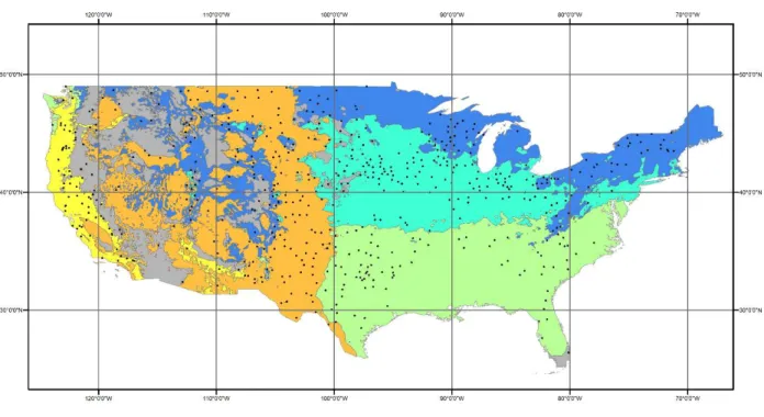
study to group the gauges. The climates used were the “BS” or steppe classification that covers the flat, un-forested land that is primarily east of the Rocky Mountains, it is most of the Great Plains. The “CF” or temperate classification, is mainly the southeastern United States that spans from part of Texas to the Chesapeake Bay. The “CS” or Mediterranean classification is primarily the west coast of the country, encompassing the entire coast of California. The last two classifications incorporated into the study were “DFA” and “DFB”. DFA refers to cold areas with hot summers, and DFB is cold areas with warm summers. DFA is directly above the CF climatic area consisting of the central part of the United States, encompassing the area east of the Great Plains to the Atlantic coast. The DFB area is immediately north of this, spanning all of New England, as well as a small patch of the Appalachian Mountains.
2.2 Rain Gauge Data
The source of rain gauge data in this study was the Cooperative Observers Program Hourly Precipitation Dataset of NOAA (National Centers for Environmental Information, 2017). This dataset contains 1920 gauges that cover the CONUS with varying records, with some dating back up to 1948. Supplementary to the quality check done by NOAA, the authors conducted further quality assurance for the study. Stations needed to have at least 50 full years of data recorded. For a year to be counted as a full year, the record needed to contain more than 80% of the available hours in that year (Barbero et al., 2017; Marra et al., 2017). Once the gauges that met this criterion were selected, the annual maximum series for 1- and 24-hour durations for each gauge had to be stationary at a 0.1 significance level. After this quality checking process was complete, 582 gauges were identified as available for the study. Figure 1 shows the final dataset of gauges used in the study that met the quality checking benchmarks within the Koppen-Geiger climatic classification developed by Peel et al. (2007). Due to the low number of gauges within the “BW” (desert) and
6
“Other” class defined by Peel et al., 2007, the 43 gauges between those climatic regions were removed as well. This left 539 gauges that were referred to as “valid” gauges. The five main classes used to divide the gauges were: BS (steppe, 139 gauges), CF (temperate, 88 gauges), CS (Mediterranean, 53 gauges), DFA (Cold; hot summer, 140 gauges) and DFB (cold; warm summer, 119 gauges).
Figure 1: Map of CONUS showing: (i) Koppen-Geiger climatic classification groups included in the study, from Peel et al. (2007); (ii) location of the NOAA HPD rain gauges with 50+ years with 80%+ available hourly data
2.3 Radar Data
The radar-rainfall data is retrieved from a national network of S-band Doppler weather radar stations. This is known as the Next-Generation Radar (NEXRAD) network.
7
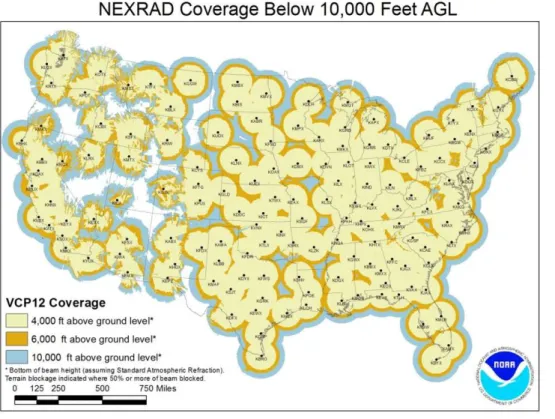
In this analysis, the radar product used was the NEXRAD Stage IV data. Stage IV is a nationally mosaicked, gauge-corrected and river forecasts centers manual quality controlled radar product. Stage IV provides a 4km grid resolution estimate of 1-hour rainfall intensity. The NEXRAD coverage map is shown in figure 2. For this study we used the entire available hourly record of Stage IV product (2002 – 2017) over CONUS and further selected 582 pixels that corresponded with the valid rain gauges being used in the study.
Figure 2:NEXRAD coverage area across the CONUS (Source NOAA)
3. Methods
The analysis was broken into a two-step evaluation. The first step was a climate-zone wide quantile - quantile comparison of annual maxima series at each duration. After this, the IDFs were derived for the NEXRAD Stage IV data and the corresponding gauge data at the valid gauge locations, and
8
grouped into their climate groupings for evaluation of the radar IDFs in comparison with the gauge IDFs.
3.1 Quantile-Quantile Comparison
The initial step was to compare the AMS quantiles from the data sources qualitatively in quantile-quantile density plots for the entire climatic zone. The annual maxima series from all three data sources at each location was normalized by the mean. The Q-Q density plotting was done for the NEXRAD Stage IV quantiles versus the full gauge record quantiles. To ultimately ensure that the AMS from NEXRAD, full gauge record, and overlapping “short” gauge record all came from the same distribution, the Q-Q density plotting was also done for the 16-year gauge record that overlaps with the NEXRAD Stage IV data versus the full gauge record. Along with this, the distribution of the mean ratios from the normalization were also done, showing the distribution of the individual mean values from NEXRAD Stage IV over the full gauge record and the distribution of the individual mean values from the short gauge record over the full gauge record.
3.2 Rainfall Frequency Analysis Methods
This section describes the method used for rainfall frequency analysis. The annual maxima series (AMS) approach of extreme value theory due its simplicity and ease of the application in frequency analysis, as well as being a commonly used approach. The AMS approach involves taking the annual maximum average intensity for 1-, 3-, 6-, 12-, and 24-hour durations from 16-year NEXRAD Stage IV time-series and the earliest 50 years from the rain gauge records for each pixel-gauge pairing. It should be noted that the quality checking process took the most recent, “full” 50 years of record from the rain gauges.
Common with other works involving extreme event analysis, the generalized extreme value (GEV) distribution was used to fit the annual maxima series. The GEV distribution is an extreme value
9
distribution consisting of three parameters commonly used to model rainfall extremes (Fowler and Kilsby, 2003; Gellens, 2002; Koutsoyiannis,2004; Overeem et al., 2008). According to the gauge-based Precipitation Frequency analysis conducted for NOAA Atlas 14, the GEV distribution consistently fit the data better than other extreme value distributions (Perica et al., 2013). The GEV is also widely used for extreme rainfall statistical analysis based on remote sensing data, including radar (Eldardiry et al., 2015; Marra and Morin, 2015; Overeem et al.,2009; Panziera et al., 2016; Marra and Morin, 2017). The three parameters comprising the GEV distribution stem from the combination of the Gumbel, Frechet, and Weibull models. The GEV is described by the location, scale, and shape parameters, which represent mean, dispersion and skewness of the distribution. The cumulative distribution function (CDF) of the GEV is shown below:
𝐹(𝐼; 𝜇, 𝜎, 𝜅) = exp − 1 +𝜅
𝜇(𝐼 − 𝜇) , 𝑓𝑜𝑟 𝜅 ≠ 0
𝐹(𝐼; 𝜇, 𝜎, 𝜅) = exp − exp −1
𝜎 (𝐼 − 𝜇) , 𝑓𝑜𝑟 𝑘 = 0
In this work, we used the method of linear moments (L-moments, LMOM) for GEV parameter estimation. This method provides improved estimates of the GEV-distribution parameters in situations with short data records and it is also less sensitive to outliers in comparison to the Maximum Likelihood method (Martins and Stedinger, 2000). This is advantageous for this study, as we are deriving GEV parameters for the generation of IDFs with 16 years of radar data. Radar-Derived IDFs: A GEV distribution was fitted to the individual radar AMS. The modeled distribution was used to derive the NEXRAD-based estimates of 2-, 5-, 15-, 25-, 50-, and 100-year return periods at five different durations of 1 hour, 3 hours, 6 hours, 12 hours, and 24 hours.
10
Gauge-Derived IDFs: The baseline for this work was the gauge-derived IDFs for the same record length as the available NEXRAD Stage IV data (16 years). To establish the uncertainty as a basis for comparison with the radar-derived IDFs, a GEV distribution was fit to a synthetic 16-year AMS sample that was sampled with replacement from the original 50-year sample at an individual gauge. This process was bootstrapped 1000 times yielding 1000 gauge-based estimates of 2-, 5-, 15-, 25-, 50-, and 100-year return periods at all 5 durations. For each gauge, the median as well as the 5th and 95th confidence bounds were found for the comparison with the NEXRAD-based IDFs. This process is similar to the operation performed by Marra and Morin, 2017 as well as Overeem et al., 2009.
3.3 Radar-based IDF evaluation Metrics
To evaluate the radar-based IDF’s estimation accuracy relative to the short record-based gauge IDF, two main metrics were used, the exceedance probability and delta. Exceedance probability was the number of times a NEXRAD intensity value exceeded the confidence bounds of the gauge intensity at each return period for a given duration. This was done at each climate group scale. Delta is a distance-based metric designed to quantify the amount of uncertainty of the NEXRAD IDF relative to the amount of uncertainty that exists from the gauge IDF. This is conducted for each return period of interest at every duration. Delta takes into account the difference in intensity between the gauge-based IDFs median intensity from the bootstrapping analysis and the NEXRAD based intensity. The use of delta is to go beyond a binary metric as it provides both radar estimates that may have exceeded the confidence bounds as well as radar estimates that were very comparable. Equations demonstrating these metrics are show below, as well as Figure 3 which shows an example of the comparison of NEXRAD Stage IV and gauge based IDFs.
11
𝑃 = 𝑁
𝑁
Where 𝑁 = Number of exceedances for given return period, 𝑁 = Number of gauges in climatic grouping
𝛿 =𝐼 − 𝐼
1
2(𝐼 − 𝐼 )
Where 𝐼 = Intensity from NEXRAD for given return period, 𝐼 = Median intensity from gauge for given return period, 𝐼 , 𝐼 = Intensity of 95th and 5th confidence interval.
12
Figure 3: Example of NEXRAD vs Gauge based IDFs. Red line represents the NEXRAD IDF estimate and the thick blue line the median gauge IDF estimate. The shaded area represents the 5-95 gauge-based IDF confidence bounds from the bootstrapping exercise. The 1-,3-, 6-, & 12-hour IDF curves are shown to help demonstrate the evaluation metrics
4. Results and Discussion
This section presents the results of the work. The first part presents the results of the quantile-quintile (QQ) comparison. The second part presents the results of comparison of NEXRAD Stage IV and gauge derived IDFs.
13
4.1 Quantile-Quantile Comparison
14
15
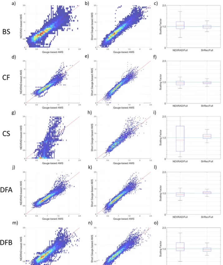
The first column of plots in figure 4 (a, d, g, j, and m) display the quantile-quantile density plots comparing the NEXRAD Stage IV AMS values with the full record gauge based AMS values within the climate zones listed adjacent to the plots. The second column of plots in figure 4 (b, e, h, k, and n) display the quantile-quantile density plot comparing the overlapping, 16-year, “shortened” gauge AMS compared with the same full gauge record AMS as used on the X-axis of the first column. The third and final column (c, f, I, l, and o) displays the distribution of the ratios of the mean values used when normalizing the data that went into the quantile-quantile plots. For the BS, CF, DFA, and DFB climate zones, the density plots in the first column have similar shape to the second column density plots. However, in general, the NEXRAD vs gauge-based density plots tend to show a larger spread of values than the shortened gauge versus longer gauge. At the smaller quantiles NEXRAD seems to underestimate the gauge rainfall AMS values. As well as a good agreement in the density plots, the third column for these climate zones show the median of the scaling factors to be close to 1 for the two data sources, with the confidence interval being within 0-2 for both data sources. However, the ratios of the two gauge-based datasets tend to have a smaller amount of uncertainty than the NEXRAD/full record ratios.
The CS climate zone, unlike the other groupings in the study, displays very poor shape of the quantile-quantile density plot comparing the NEXRAD-based AMS with the full record gauge-based AMS. Plots 4g and 4h do not have similar shape. Plot 4c shows the median of the scaling factor for the short/full gauge to be close to 1. Due to the agreement in shape of the CS groupings density plot in the second column with the rest of the second column, plot 4g shows the problems faced with radar quantitative precipitation estimates on the west coast of the United States and areas of complex terrain, a known problem with the NEXRAD radar network observations and precipitation retrievals (Westrick et al., 1999; Matrosov et al., 2014).
16
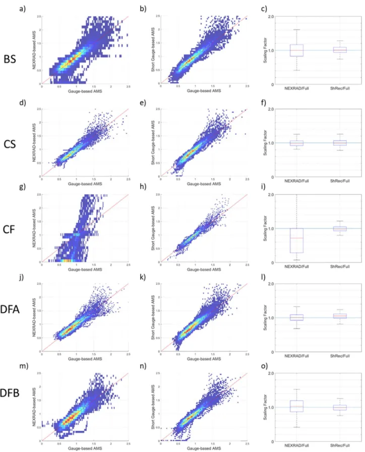
For the 12-hour duration plots show in figure 5, the NEXRAD Stage IV AMS quantile plots in 5a, 5d, 5j, and 5m appear more compact than their 1-hour counter parts, especially along the 45 degree reference line. With this, the median values in 5c, 5f, 5l, and 5o are all almost directly at the value of 1 shown by the blue reference line. The CS climate continues to show systematic radar rainfall estimation issues as previously mentioned.
Overall, with the exception of the CS climate zone, the NEXRAD AMS quantiles were comparable to those from the full gauge record. Also, the NEXRAD AMS quantiles come from the same distribution as the 16-year gauge record quantiles. Based on these results for the 1 and 12 hour duration QQ plots. The authors proceeded to use the Stage IV data to generate IDFs without conducting adjustments to the available data.
17
4.2 Evaluation Metrics
18
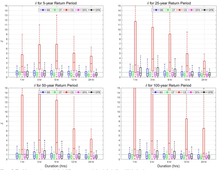
Figure 7: The delta uncertainty metric for 4 different return periods at 1-,3-,6-,12-, and 24-hr durations
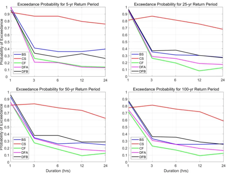
The 5-year return period results are shown in plots 6a and 7a. The 5-year exceedance probability for 1-hour duration is almost completely exceeded across all climate zones. However, as soon as the duration is increased to 3-hours, there is a substantial drop in exceedance. This trend is shown across all the return periods analyzed. The only climate grouping that doesn’t experience a decrease in exceedance probability is the CS climate group, which consistently shows a large amount of exceedance across the four return periods presented. In contrast, the CF and DFA climatic regions consistently have the lowest exceedance probability. These climate zones perform
19
very well in the shorter return periods, with both less than 30% exceedance at durations over 3-hours, highlighted in figure 6a.
Along with the high exceedance probability for the 1 hour duration, the delta values at this duration yield that while some NEXRAD IDFs were close to the median gauge IDF, there were values greater than 4-6 times the size of the uncertainty area for the given return periods (delta uses ½ in the denominator). However, the median values for BS, CF, DFA, and DFB all fall within the reference line at 1, which we can theoretically assume to be within the uncertainty bounds based on the delta equation. Predictably, the exceedance probability for the 5-year return period at longer durations such as 12-and 24-hour, are low, as well as the magnitude of the delta values.
Figures 6b and 7b display the exceedance probability and delta values for the 25-year return period. The exceedance probabilities display almost complete exceedance at the 1-hour duration. However, similar to the 5-year return period, moving forward to the 3-hour duration sees a large decrease in exceedance across all climate groupings except the CS. At the 6-hour duration there is a slight increase in exceedance of the DFA climate group, this may be due to the diverse swath of land covered by this climate grouping, incorporating parts of the mid-Atlantic as well as the Great Plains. The delta metric at the 25-year return period is highlight a slight downward or consistent trend in the median values of the same durations from the 5-year return period shown in figure 6a. The exceedance probability and delta metrics for the 50-year return period are shown in figure 6c and 7c. At the 50-year return period the BS climate group has similar results to the CF and DFA climate groups especially for the 3- and 6-hour durations. At the 24-hour duration, all climate groups except for the CS group are under 40% exceedance.
20
The 100-year return period exceedance probability and delta metric results are shown in figures 6d and 7d. The exceedance probabilities for the five durations examined in this study follow a similar trend as the shorter three return periods highlighted. The delta results at this duration show the further overall reduction in the median values of the 4 non-problematic climate zones. Some of this is related to the equation used for this metric. Because of the large size of the confidence bounds, the denominator of the delta equation is quite large. This is part of why the reduction in delta and the overall distribution of delta for each climate zone is seen, even at the 1-hour duration. The DFB climate zone had some large delta values within it, however, the median at all durations was less than 1.0, as well as the 75th quantile at the 24 hour duration. Consistent with the lesser
return periods analyzed, the median as well as distribution of values from the CF climate zone saw small reductions do the already small distribution and magnitude of delta values. The DFA climate zone delta median is also consistently under the 1.0 theoretical threshold value, and with the exception of the 3-hour duration, the 75th quantile is also under the 1.0 theoretical value.
The four exceedance probability subfigures show us that at the 1-hour duration, there is systematic exceedance of the NEXRAD-derived IDF across all climatic groupings. However, for the 5-year return period, as soon as the duration is increased to 3-hours, there is a substantial drop in exceedance. This trend is shown across all the return periods analyzed. The only climate grouping that doesn’t experience a decrease in exceedance probability is the CS climate group, which consistently shows a large amount of exceedance across the four return periods presented. In contrast, the CF and DFA climatic regions consistently have the lowest exceedance probability. Along with the high exceedance probability for the 1 hour duration, the delta values at this duration yield that while some NEXRAD IDFs were close to the median gauge IDF, there were values greater than 4-6 times the size of the uncertainty area for the given return periods (delta uses ½ in
21
the denominator). However, the median values for BS, CF, DFA, and DFB all fall within the reference line at 1, which we can theoretically assume to be within the uncertainty bounds based on the delta equation.
At 1-hour duration for all return periods, there is the largest amount of exceedance and magnitude of delta values present. However, with increasing return period, especially at 3-hour duration and higher, the magnitude of the delta values decreases as does the exceedance probability. This is due to both an increase in uncertainty for the gauge based IDF’s. Another reason for the improved performance of longer durations compared to 1-hour is from the temporal averaging that is done to extract the annual maximum average intensity over longer durations. Of course, this could also be due to the Stage IV data’s ability to provide accurate rainfall estimates at longer durations. The NEXRAD derived IDF’s in the CS climate are systematically over for all durations at all return periods. This is a reflection of the discrepancies in AMS values between the NEXRAD data and rain gauge data that has been previously discussed. This is why in for all included evaluation metrics, the CS (red in the figures) appears to be problematic. This can be expected based on previous research of challenges faced by NEXRAD in complex terrain and coastal areas, primarily due to beam blockage and beam overshoot (National Research Council, 2005).
5. Conclusions
This study expanded on previous radar-based extreme rainfall statistical derivation by attempting to evaluate the potential ability of NEXRAD Stage IV data to derive sub-daily IDFs for ungauged locations. A numerical experiment was conducted to compare the radar derived IDF values to the variability that exists in estimating IDFs using a gauge record over the same 16 year period.
22
IDFs were calculated by bootstrapping and fitting the GEV distribution to 16-year annual maxima series from 539 hourly rain gauges representing different climates in the CONUS. The gauges had at least 50 years of data with 80% of data coverage within each available year. The radar-based IDF curves were compared to the corresponding gauge-based IDF by calculating the exceedance probability and uncertainty ratio of the NEXRAD IDF relative to the confidence bounds of the gauge IDF. The IDF curves were focused on return periods of 2, 5, 10, 25, 50, and 100-years. Based on the quantile-quantile assessment of annual maxima series from NEXRAD and rain gauge data sources, NEXRAD tends to overestimate intensity at shorter durations (1-,3-hr), while it tends to overestimate intensity at longer durations (12-,14-hr).
The NEXRAD-based IDFs systematically exceed the uncertainty bounds of the gauge-derived IDFs in all climatic zones at the 1-hour duration. As well as high exceedance probabilities, the delta values for all climates are high, especially for smaller return periods due to the small amount of uncertainty. However, with increasing duration, the BS, CF, DFA, and DFB climate zones seen a reduction in exceedance and a convergence in the delta metric, including for smaller return periods.
This study demonstrates the ability of the NEXRAD Stage IV data to provide comparable derived IDF relationship values for durations greater than 1-hour. It is therefore our belief that Stage IV data provides the ability to yield reliable IDF results in ungauged locations.
Future research should continue to evaluate the Stage IV data’s ability to derive IDFs as its available historical record increases. Other possible considerations for future research could be comparing NEXRAD-based IDFs with NOAA’s Atlas-14 to evaluate the potential to provide accurate sub-daily IDFs in place of Altas-14’s interpolation methods.
23
References
A, James Wesley P. Wurbs Ralph. Water Resources Engineering Wurbs- International Edition. Prentice-Hall, 2002.
Eagleson, P. S., Dynamic Hydrology, McGraw-Hill, New York, 462p., 1970., n.d.
Eldardiry, Hisham, Emad Habib, and Yu Zhang. “On the Use of Radar-Based Quantitative Precipitation Estimates for Precipitation Frequency Analysis.” Journal of Hydrology, Hydrologic Applications of Weather Radar, 531 (December 1, 2015): 441–53. https://doi.org/10.1016/j.jhydrol.2015.05.016.
Froot, Kenneth, ed. The Financing of Catastrophe Risk. A National Bureau of Economic Research Project Report. Chicago: University of Chicago Press, 1999.
Hosking, J. R. M. “L-Moments: Analysis and Estimation of Distributions Using Linear Combinations of Order Statistics.” Journal of the Royal Statistical Society. Series B
(Methodological) 52, no. 1 (1990): 105–24.
Kidd, Chris, Andreas Becker, George J. Huffman, Catherine L. Muller, Paul Joe, Gail
Skofronick-Jackson, and Dalia B. Kirschbaum. “So, How Much of the Earth’s Surface Is Covered by Rain Gauges?” Bulletin of the American Meteorological Society 98, no. 1 (June 6, 2016): 69–78. https://doi.org/10.1175/BAMS-D-14-00283.1.
Marra, F., E. Morin, N. Peleg, Y. Mei, and E. N. Anagnostou. “Intensity–duration–frequency Curves from Remote Sensing Rainfall Estimates: Comparing Satellite and Weather Radar over the Eastern Mediterranean.” Hydrol. Earth Syst. Sci. 21, no. 5 (May 9, 2017): 2389– 2404. https://doi.org/10.5194/hess-21-2389-2017.
National Centers for Environmental Information (2017), Cooperative Observers Program Hourly Precipitation Dataset (C-HPD), Version 2.0 Beta, NOAA National Centers for Environmental Information. [accessed January 11, 2018]
National Research Council. “Flash Flood Forecasting Over Complex Terrain: With an
Assessment of the Sulphur Mountain NEXRAD in Southern California” at NAP.Edu.
Accessed April 10, 2018. https://doi.org/10.17226/11128.
Nikolopoulos, E. I., M. Borga, J. D. Creutin, and F. Marra. “Estimation of Debris Flow Triggering Rainfall: Influence of Rain Gauge Density and Interpolation Methods.”
Geomorphology 243 (August 15, 2015): 40–50.
https://doi.org/10.1016/j.geomorph.2015.04.028.
Nikolopoulos, Efthymios I., Stefano Crema, Lorenzo Marchi, Francesco Marra, Fausto Guzzetti, and Marco Borga. “Impact of Uncertainty in Rainfall Estimation on the Identification of Rainfall Thresholds for Debris Flow Occurrence.” Geomorphology 221 (September 15, 2014): 286–97. https://doi.org/10.1016/j.geomorph.2014.06.015.
NOAA, “Atlas14 Volume2.Pdf.” Accessed March 6, 2018.
http://www.nws.noaa.gov/oh/hdsc/PF_documents/Atlas14_Volume2.pdf.
Overeem, A., Buishand, T. A., and Holleman, I.(2009), Extreme rainfall analysis and estimation of depth–duration–frequency curves using weather radar, Wate Resour. Res., 45, 10424, doi:10.1029/2009WR007869
Peel, M. C., B. L. Finlayson, and T. A. Mcmahon. “Updated World Map of the Köppen-Geiger Climate Classification.” Hydrology and Earth System Sciences Discussions 11, no. 5 (October 2007): 1633–44.
Sivapalan, Murugesu, and Günter Blöschl. “Transformation of Point Rainfall to Areal Rainfall: Intensity-Duration-Frequency Curves.” Journal of Hydrology 204, no. 1 (January 30, 1998): 150–67. https://doi.org/10.1016/S0022-1694(97)00117-0.
24
Watt, Ed, and Jiri Marsalek. “Critical Review of the Evolution of the Design Storm Event Concept.” Canadian Journal of Civil Engineering 40, no. 2 (February 1, 2013): 105–13. https://doi.org/10.1139/cjce-2011-0594.
Wright, Daniel B., James A. Smith, Gabriele Villarini, and Mary Lynn Baeck. “Estimating the Frequency of Extreme Rainfall Using Weather Radar and Stochastic Storm
Transposition.” Journal of Hydrology 488 (April 30, 2013): 150–65. https://doi.org/10.1016/j.jhydrol.2013.03.003.