City, University of London Institutional Repository
Citation: Fring, A. and Dey, S. (2014). Noncommutative quantum mechanics in a
time-dependent background. Physical Review D - Particles, Fields, Gravitation and Cosmology, 90, 084005 -084019. doi: 10.1103/PhysRevD.90.084005This is the accepted version of the paper.
This version of the publication may differ from the final published
version.
Permanent repository link: http://openaccess.city.ac.uk/4150/
Link to published version: http://dx.doi.org/10.1103/PhysRevD.90.084005
Copyright and reuse: City Research Online aims to make research
outputs of City, University of London available to a wider audience.
Copyright and Moral Rights remain with the author(s) and/or copyright
holders. URLs from City Research Online may be freely distributed and
linked to.
City Research Online: http://openaccess.city.ac.uk/ [email protected]
Noncommutative quantum mechanics in a
time-dependent background
Sanjib Dey and Andreas Fring
Department of Mathematics, City University London, Northampton Square, London EC1V 0HB, UK E-mail: [email protected], [email protected]
A : We investigate a quantum mechanical system on a noncommutative space for which the structure constant is explicitly time-dependent. Any autonomous Hamil-tonian on such a space acquires a time-dependent form in terms of the conventional canonical variables. We employ the Lewis-Riesenfeld method of invariants to construct explicit analytical solutions for the corresponding time-dependent Schrödinger equation. The eigenfunctions are expressed in terms of the solutions of variants of the nonlinear Ermakov-Pinney equation and discussed in detail for various types of background fields. We utilize the solutions to verify a generalized version of Heisenberg’s uncertainty rela-tions for which the lower bound becomes a time-dependent function of the background fields. We study the variance for various states including standard Glauber coherent states with their squeezed versions and Gaussian Klauder coherent states resembling a quasi-classical behaviour. No type of coherent states appears to be optimal in general with regard to achieving minimal uncertainties, as this feature turns out to be background field dependent.
1. Introduction
The study of quantum mechanics and quantum field theories on noncommutative space-time structures is motivated by the fact that it achieves gravitational stability [1] in almost all currently known approaches to quantum gravity, such as string theory [2, 3, 4] or loop quantum gravity [5, 6]. In a quantum mechanical setting the most commonly studied version of these space-time structures consists of replacing the standard set of commu-tation relations for the canonical coordinates xµ by noncommutative versions, such as
explicit time-dependence in θµν. Although various effective Lagrangians for such type of noncommutative field theories have been derived, e.g. [12], little is known about explicit quantum theories on such type of spaces, one of the reasons being that they are far more difficult to solve.
Here our aim is to find explicit solutions for a simple prototype quantum mechanical model on a time-dependent background and study the physical consequences such a space will imply. We focus here on the particular two-dimensional space with nonvanishing commutators for the coordinatesX,Y and momentaPx, Py
[X, Y] =iθ(t), [Px, Py] =iΩ(t), [X, Px] = [Y, Py] =i +iθ(t)Ω(t)
4 , (1.1)
where the noncommutative structure constants θ(t) and Ω(t) are taken to be real valued functions of timet. Of course a multitude of other possibilities exists. The specific form presented here allows for an elegant representation, as we shall see in detail below. When considering representations for these phase-space variables one is inevitably lead to time-dependent Hamiltonians H(X, Y, Px, Py)→H(t).
We will employ here the method of invariants, introduced originally by Lewis and Riesenfeld [13], to solve the time-dependent Schrödinger equation
i ∂t|ψn =H(t)|ψn , (1.2)
for the time-dependent or dressed states |ψn associated to the HamiltonianH(t).
Let us briefly describe the key steps of the method for future reference. The initial step in that approach consists of constructing a Hermitian time-dependent invariant I(t)
from the evolution equation
dI(t)
dt =∂tI(t) +
1
i [I(t), H(t)] = 0. (1.3)
In the next step one needs to solve the corresponding eigenvalue system involving the invariant
I(t)|φn =λ|φn , (1.4)
for real and time-independent eigenvalues λ and for time-dependent states |φn . It was shown in [13] that the states
|ψn =eiα(t)|φn (1.5)
satisfy the time-dependent Schrödinger equation (1.2) provided that the real functionα(t)
in (1.5) obeys
dα(t)
dt =
1
φn|i ∂t−H(t)|φn . (1.6)
commutation relations (1.1). Following standard arguments, the uncertainty for the simul-taneous measurement of the observables Aand B has to obey the inequality
∆A∆B|ψ ≥
1
2| ψ|[A, B]|ψ |, (1.7)
with ∆A|2ψ = ψ|A2|ψ − ψ|A|ψ
2 and similarly for
B for any state |ψ . Evidently, for instance the first relation in (1.1) implies that the uncertainty for the simultaneous measurement ofX and Y is greater than the function of time |θ(t)|/2 rather than simply being greater than a constant. Of special interest is to see whether the time-dependent bound can be saturated by the use of various types of coherent states in (1.7).
Our manuscript is organized as follows: In section 2 we construct the time-dependent invariant I(t) for the two dimensional harmonic oscillator on the background described by (1.1). We compute its time-dependent eigenfunctions |φn , determine the phase α(t) thereafter and hence the eigenstates |ψn of H(t). As all solutions are dependent on the solutions of the nonlinear Ermakov-Pinney equation we devote section 3 to a discussion of its solutions. In section 4 we assemble the solutions from section 2 and 3 to investigate the validity and quality of a generalized version of Heisenberg’s uncertainty relations. Partic-ular focus is placed on the study of the uncertainty relations when computed with regard to standard Glauber coherent states, including their squeezed versions and also Gaussian Klauder coherent states. In section 5 we state our conclusions.
2. The 2D harmonic oscillator in a time-dependent background
The main features of models on time-dependent backgrounds can be explained by consid-ering simple two dimensional models. Therefore we will examine here as prototype two dimensional model the harmonic oscillator of the form
H(X, Y, Px, Py) = 1 2m P
2
x +Py2 + mω2
2 (X
2+Y2), (2.1)
on the noncommutative space (1.1). From the many possibly representations, we choose here a Hermitian one obtained from standard Bopp-shifts in the conventional canonical variablesx,y,px and py, with nonvanishing commutators[x, px] = [y, py] =i , as
X=x− θ2(t)py, Y =y+θ(t)
2 px, Px=px+ Ω(t)
2 y, Py =py− Ω(t)
2 x. (2.2)
As anticipated, when converting the Hamiltonian in (2.1) to the standard variables it becomes explicitly time-dependent
H(t) =1 2a(t) p
2
x+p2y +
1 2b(t) x
2+y2 +c(t) (pxy−xpy) (2.3)
with coefficients
a(t) = 1
m+ mω2
4 2 θ
2(t), b(t) =mω2+Ω2(t)
4m 2, c(t) =
mω2θ(t)
2 +
Ω(t)
We notice that forθ(t) = 0we can view this Hamiltonian with an appropriate identification of the remaining functions as describing a particle with mass m moving in an axially symmetric electromagnetic field, see section IV in [13]. It should also be noted that with a re-definition of the time-dependent coefficient attempts to solve the eigenvalue problem related to (2.3) can be found in the literature [14, 15]. Unfortunately the solutions provided are partly incorrect or not useful for our purposes as we shall be commenting on below in more detail.
The quantum equations of motion for the canonical variables associated to the Hamil-tonian (2.3) are simply
˙
x = 1
i [x, H] =a(t)px+c(t)y, y˙=
1
i [y, H] =a(t)py−c(t)x, (2.5)
˙
px = 1
i [px, H] =−b(t)x+c(t)py, py˙ =
1
i [py, H] =−b(t)y−c(t)px, (2.6)
where we adopt the usual convention for the time derivative∂tf =: ˙f.
2.1 Construction of time-dependent invariants
A non-Hermitian invariant is constructed right away, by following the argumentation al-ready provided in [13]. Defining the non-canonical variables
Q:= (x+iy)ei tc(s)ds and P := (px+ipy)ei tc(s)ds, (2.7)
satisfying[Q, P] = 0, we find with (2.5) and (2.6) the same equations of motion for these variables
˙
Q=a(t)P and P˙ =−b(t)Q. (2.8)
as for the harmonic oscillator with a time-dependent mass term [16]. This is all that matters for the identification of a formal invariantI˜(t) in terms of the variablesQ andP
˜
I(t) = 1 2
τ σ2Q
2+ (σP −σ˙
aQ)
2 = ˜I†(t), (2.9)
since we may simply take the expression from the literature and adapt the relevant quan-tities appropriately. Here σ is a new auxiliary quantity that has to satisfy a nonlinear Ermakov-Pinney (EP) [17, 18] equations including a dissipative term
¨
σ−aa˙σ˙+abσ=τa
2
σ3, (2.10)
with integration constantτ. It is well-known that variations of this equation are ubiquitous in this context of solving time-dependent Hamiltonian systems, see for instance equation (5) in [19], which reduces exactly to (2.10) forA→a,B→0andC →τ and [21, 22, 23, 24] for variations of this equation. Note that σ = 0 implies that a = 0, which is impossible according to (2.4), such that we can devide byσ without any further concern.
In principle the fact thatI˜in (2.9) is an invariant means I˜I˜† or I˜†I˜constitute
directly suitable to an operator approach to find the corresponding eigensystems we seek an additional one of lower order in the canonical variables, having however equation (2.10) in common.
The symmetry of the Hamiltonian suggest to carry out a quantum canonical transfor-mation using polar coordinates x=rcosθ, y=rsinθ, which indeed turns out to be very suitable. The canonical coordinates and momenta are thenr = x2+y2,θ= arctan(y/x)
and pr = (xpx+ypy)/r−i /(2r), pθ =xpy−ypx, such that the canonical commutation relations are [r, pr] = [θ, pθ] = i . The last term in pr is not essential for the canonical commutation relations, but its inclusion ensures the Hermiticity of pr and leads to the convenient identity p2x+p2y = p2r+p2θ/r2 − 2/(4r2) allowing to convert the Hamiltonian (2.3) into the form
H(t) = 1
2a(t) p 2
r+ p2
θ r2 −
2
4r2 + 1 2b(t)r
2
−c(t)pθ. (2.11)
Applying now the Lewis-Riesenfeld method of invariants and construct a Hermitian time-dependent invariantI(t) by using (1.3), we commence with the standard assumption that the invariant is of the same order and form in the canonical variables as the original Hamiltonian. Similarly as the Hamiltonian, we assume here that also the invariant does not depend explicitly on θand take it to be of the general form
I(t) =α(t)p2r+β(t)r2+γ(t){r, pr}+δ(t)p 2
θ r2 +ε(t)
pθ r2 +φ(t)
1
r2, (2.12)
with unknown time-dependent coefficients α(t),β(t), γ(t) etc. The substitution of (2.12) into (1.3) then yields the following constraints on these coefficients
˙
α=−2aγ, β˙ = 2bγ, γ˙ =bα−aβ, (2.13)
˙
δp2θ+ ˙εpθ+ ˙φ= 2aγ−2aγpθ2, (δ−α)p2θ+εpθ+φ+ α 2
4 = 0. (2.14)
We observe that the equations in (2.13) take on the same form as the equations underlying the explicit construction for the time-dependent harmonic oscillator [16]. They can be solved by parameterizing α(t) =σ2(t) and after one integration we are led exactly to the
nonlinear Ermakov-Pinney equations (2.10) underlying the solution for our non-Hermitian invariant I˜(t). The remaining equations (2.14) are consistently solved by
δ=α, ε= 0, and φ=−α
2
4 . (2.15)
Assembling everything, the Hermitian invariantI(t) for the time-dependent Hamiltonian (2.3) then acquires the form
I(t) = τ
σ2r
2+ σpr−σ˙
ar
2 +σ
2p2
θ r2 −
σ2 2
4r2 , (2.16)
with σ(t) determined by the Ermakov-Pinney equation (2.10). As argued already in [13] the arbitrary constantτ may be scaled away, thus that from now on we simply set it to 1
Next we solve the eigenvalue equation (1.4) by expressing the invariantI(t) in terms of time-dependent creation and annihilation operators
ˆ
a(t) = 1
2√ σpr−
˙
σ ar −i
r σ +
σ
r(pθ+ 2) e
−iθ, (2.17)
ˆ
a†(t) = 1 2√ e
iθ σpr−σ˙ ar +i
r σ +
σ
r(pθ+2) , (2.18)
satisfying[ˆa,aˆ†] = 1, by means of the identity
ˆ
a†ˆa+ 1
2 −pθ= 1 4I(t)−
1
2pθ =: ˆI(t). (2.19)
ClearlyIˆ(t) is also an invariant, where the factor 1/4 simply amounts to a new value for the integration constantτ and pθ may be added toI(t) since[H(t), pθ] = 0.
2.2 Eigensystem for the time-dependent invariant
We can now employ the standard argumentation from [13] to construct the eigenstates and eigenfunctions for the invariant Iˆ(t). Noting first that [ ˆI(t), pθ] = 0, one concludes that
ˆ
I(t)and pθ possess simultaneous eigenvectors, say |n, ℓ , with
ˆ
I|n, ℓ = n+ 1
2 |n, ℓ , pθ|n, ℓ = ℓ|n, ℓ , n, ℓ|n, ℓ = 1. (2.20)
Computing therefore n, ℓ|ˆa†ˆa|n, ℓ = n+ℓ ≥ 0 implies that for given n we have ℓ ∈
{−n, . . . ,0,1,2, . . .}. The eigenstates of this sequence therefore obey
ˆ
a|n,−n = 0, |n, m−n = √1
m! ˆa † m
|n,−n , with n, m∈N0. (2.21)
For all observables that can be expressed in terms of the time-dependent creation and annihilation operatorsaˆ† and ˆa, we can simply use operator techniques to compute their expectation values. However, the former is not possible for our observablesX,Y,Px and Py. We therefore use the explicit representations in coordinate space pθ = −i ∂θ and pr =−i [∂r+ 1/(2r)]to compute the eigenstates. Assuming now r, θ|n, ℓ =ψn,ℓ(r, θ) = ϕn(r)eiℓθ we have the desired property pθψ
n,ℓ(r, θ) = ℓψn,ℓ(r, θ). For givenn, the lowest states are then found from solving the differential equation ˆaψn,−n(r, θ) = 0, that is
ie−iθ−iθn
2arσ√ a nσ
2−ar2+ir2σσ ϕ˙ (r)−a rσ2∂rϕ(r) = 0. (2.22)
The solution to (2.22) is then easily found to be
ψn,−n(r, θ) =λnrne−
r2(a−iσσ˙)
2a σ2 e−iθn, λ2
n =
1
πn!( σ2)(1+n). (2.23)
We have fixed here the constant of integration by demanding the ground state to be nor-malized. Subsequently we construct the normalized excited states from the second relation in (2.21) to
ψn,m−n(r, θ) =λn
i 1/2σ m
√
m! r
n−meiθ(m−n)−a−iσσ˙
2a σ2r
2
U −m,1−m+n, r
2
with U(a, b, z) denoting the confluent hypergeometric function. The orthonormality rela-tion 02πdθ 0∞dr rψ∗n,m−n(r, θ)ψn′,m′−n′(r, θ) =δnn′δmm′ is verified by using the standard properties of the latter function.
It should be noted here that our solution differs from those found in the literature [14, 15]. As was pointed out in [15] the solutions provided in [14] are incorrect as they lead to time-dependent eigenvalues and thus contradict the basic foundations of the Lewis-Riesenfeld theory, i.e. equation (1.4). Our solution differs also slightly from those in [15]. Moreover, in [15] the normalization constant was left undetermined, which is, however, crucial in concrete computations following below.
2.3 Eigensystem for the Hamiltonian
The last step in the Lewis-Riesenfeld procedure consists of computing the phase α(t) in (1.5) by solving the equation
˙
αn,ℓ= 1 n, ℓ|i ∂t−H|n, ℓ . (2.25)
As already argued in [13], this may be achieved by constructing a recursive equation for the right hand side of (2.25), computing some explicit expectation values, using the freedom to choose the phase for the vacuum state and a subsequent integration.
We commence by simply replacing|n, ℓ = ˆa†/√n+ℓ|n, ℓ−1 in (2.25), obtaining
n, ℓ|i ∂t−H|n, ℓ = n, ℓ−1|i ∂t−H|n, ℓ−1 + 1
n+ℓ n, ℓ−1|[ˆa, i ∂t−H] ˆa
†
|n, ℓ−1 . (2.26) Using next the expression (2.17) for the annihilation operator and the Hamiltonian in polar coordinates (2.11), we compute
[ˆa, i ∂t−H] = c(t)−σa2((tt)) ˆa, (2.27)
upon replacingσ¨ by means of the EP-equation in the form (2.10). Substitution of (2.27) into (2.26) allows for the computation of the expectation value, thus leading to the recursive equation
n, ℓ|i ∂t−H|n, ℓ = n, ℓ−1|i ∂t−H|n, ℓ−1 + c(t)−σa2((tt)) . (2.28)
We may now iterate this equation until we reach the expectation values for vacuum state n,−n|i ∂t−H|n,−n . As argued in [13], the matrix element n,−n|∂t|n,−n involves an arbitrary constant, which we conveniently choose to set to n,−n|∂t|n,−n =
n,−n|H|n,−n . Therefore we obtain the expectation value
n, ℓ|i ∂t−H|n, ℓ = (n+ℓ) c(t)− σa2((tt)) , (2.29)
allowing us to compute the phase to
αn,ℓ(t) = (n+ℓ)
t
Our result forαn,ℓ(t)differs from the phase computed in [15], where thec(s)-term is absent. We have now obtained explicit eigenfunctions for the Hamiltonian (2.1) for any time-dependent background field in terms of the solutions of the EP-equation. Mostly in the literature the analysis is abandoned at this stage and the invariants and wavefunctions are simply expressed in terms of the yet to be determined solution to the EP-equation. How-ever, for concrete computations of measurable quantities one needs to address the auxiliary problem and solve the equations explicitly for the time-dependent functions appearing in the Hamiltonian. Surprisingly little attention has been paid to this problem in the context of solving time-dependent Hamiltonian systems and therefore we will discuss the solutions of our auxiliary equation (2.10) in the next subsection.
3. The Ermakov-Pinney equation
The simplest special solution arises when taking θ(t) =const, such thata˙ = 0and conse-quently the dissipative term vanishes. For this case particular solutions were already found by Pinney [18]
σ = u21+τ a2 u22
W2, (3.1)
whereu1,u2 are the two linearly independent solutions of the equation
¨
u+ab(t)u= 0, (3.2)
and W =u1u˙2−u˙1u2 is the corresponding Wronskian.
When a˙ = 0 no general solution to (2.10) is known, although one can construct a variety of explicit solutions following the procedure proposed in [25, 26]. We briefly outline the method and use it to construct some new solutions, which we employ later on. We start by considering the ordinary differential equation of the general form
d2σ
dt2 +g(σ)
dσ
dt +h(σ) = 0, (3.3)
for which the EP-equation can be seen as a special case with the appropriate choices for g(σ) and h(σ). Introducing the new quantity η(σ) := dσ/dt, the equation (3.3) is easily converted into the first order differential equation
ηdη
dσ +g(σ)η+h(σ) = 0. (3.4)
This implies that when having solved (3.4), a solution to the original equation (3.3) can be obtained simply from inverting ση−1(s)ds=t. It can be shown by direct substitution
that (3.4) admits the solution
η(σ) =λκh(σ)
g(σ) with λ ±
κ = −
1±√1−4κ
2κ , (3.5)
if the Chiellini integrability condition [27]
d dσ
h(σ)
with κ∈R holds. Based on this we may then find exact analytical solutions for instance
by starting with a giveng(σ) and subsequently compute
η(σ) =κλκ σ
g(s)ds and h(σ) =κg(σ)
σ
g(s)ds, (3.7)
or by starting with a givenh(σ) and subsequently evaluate
η(σ) =±λκ 2κ σ
h(s)ds and g(σ) = h(σ) 2κ σh(s)ds
. (3.8)
Following this solution procedure means of course that we are not pre-selecting our back-ground fields θ(t) and Ω(t), but instead we determine them by primarily insisting on the integrability of the EP-equation. Comparing (3.4) with the EP-equation (2.10) we identify
g(σ) = −a˙
a =−∂tlna=−
2m2ω2θθ˙
4 2+m2ω2θ2, (3.9)
h(σ) = abσ−τa
2
σ3 =
4 2+m2ω2θ2 m2ω2 4 2σ4−τ θ2 −4 2τ +σ4Ω2
16 4m2σ3 . (3.10)
The virtue of this method is that it leads to exact solutions. Nonetheless, one might also be interested in concrete types of background fields for which the integrability condition (3.6) does not hold, in which case we will resort to a numerical analysis.
3.1 Non-dissipative solutions
For the special case θ(t) = const, i.e. a˙ = 0 we can simply pre-select any explicit form for Ω(t), and thereby b(t), to construct the solutions from the general formula (3.1). For instance for a(t) = α and b(t) = βeγt, α, β, γ ∈ R, i.e. θ(t) = ±2 /mω√mα−1 and
Ω(t) =±2 mβeγt−m2ω2, we solve (3.2) in terms of Bessel functions and subsequently
obtain the particular solution by means of (3.1)
σ(t) = π 2α2τ
γ2c2 1
Y2 0
2√αβeγt/2
γ +c
2 1J02
2√αβeγt/2
γ , (3.11)
with integration constant c1 ∈ R and J0, Y0 denoting the Bessel functions of first and
second kind, respectively. Similarly different solutions are easily constructed for any other explicit choice ofb(t) for which (3.2) admits a solution.
3.2 Exponentially decaying solutions
Let us now switch on the dissipative term and take a˙ = 0 by making the additional assumption g(σ) = γ ∈ R. Then the second equation in (3.7) together with the explicit
form ofh(σ) from (2.10) yields the consistency equation
κγ2σ=abσ−τa
2
σ3, (3.12)
exponentially decaying and increasing background fieldsθ(t) =±2 /mω√mαe−γt−1 and
Ω(t) =±2 mβeγt−m2ω2 corresponding to exponentially decaying solutions of the
EP-equation
a(t) =αe−γt, b(t) =βeγt, and σ(t) =µe−γt/2, (3.13)
withα,β,γ∈R, together with the constraintµ4 =τ α2/(αβ−κγ2) resulting from (3.12).
[image:11.595.86.507.338.505.2]The Chiellini constant κis not fixed at this point, but simply determined by substituting the expressions from (3.13) into (2.10), leading to κ= 1/4. A special case of our solution corresponds to the one reported in [19] where the EP-equation of the type (2.10) appears as an auxiliary equation in the solution procedure for the Caldirola-Kanai Hamiltonian [28, 29].
Notice that for our background fields the requirement thatθ(t),Ω(t)∈Rimplies that
this solution leads to cutoff timestcafter which the background field needs to be vanishing, that is t < tc = ln(mα)/γ for α, γ > 0. It should also be noted that the constraint on the constants is quite severe and one might change the overall qualitative behaviour of the solution from a decaying solution to an oscillatory behaviour when relaxing the integrability condition.
0 1 2 3 4 5
0.0 0.2 0.4 0.6 0.8 1.0 1.2 1.4
(t)
t
(a)
0 20 40 60 80 100
0 2 4 6 8 10 12
(t)
t (b)
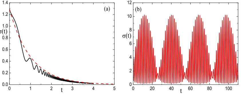
Figure 1: (a) Exactly integrable solution (3.13) (red, dashed) versus a non-Chiellini integrable solution for pre-selected exponential backgrounds θ(t) = αe−γt and Ω(t) = βeγt (black, solid).
(b) Non-Chiellini integrable solution for pre-selected sinusoidal background θ(t) = αsin(γt) and Ω(t) =βsin(γt/2). In both panels the constants are α= 5, β= 2, γ = 2, m = =τ =ω = 1,
κ= 1/4andµ= 5/3.
3.3 Rationally decaying solutions
Next we assume g(σ) =γσn withn∈N. The consistency equation then reads
κγ2σ
2n+1
n+ 1 =abσ−τ
a2
σ3, (3.14)
to the background fields and the EP-equation
a(t) = α
n+2
n
n+2
n
(γt−µ)(n+2)/n, b(t) =
β nn+2
2
n−1
(γt−µ)1−n2
, and σ(t) =
n+2
n
1
n
(γt−µ)1/n, (3.15)
with constraintγ2 = (n+ 1)(αβ−τ α2)/κ. The Chiellini constant is subsequently fixed to κ= (n+ 1)/(n+ 2)2. To maintain real solutions requires here a cutoff time t < tc =µ/γ
forγ, µ >0.
3.4 Non-Chiellini integrable solutions with pre-selected background
As pointed out, the solutions constructed in the previous subsections are special in the sense that the Chiellini integrability has been superimposed onto them. Nonetheless, given a specific background we may always find numerical solutions. In figure 1 we depict some solutions for exponential and sinusoidal background fields which we shall employ below in our solutions for the time-dependent wavefunctions.
4. The generalized uncertainty relations
4.1 The generalized uncertainty relations for eigenstates
We have assembled now all the necessary ingredients for the explicit computation of ex-pectation values. We are therefore in the position to test the generalized uncertainty relations (1.7). Having obtained explicit expressions for the wavefunctions in coordinate space, we simply use the representation in polar coordinates x = rcosθ, y = rsinθ, px = −i cosθ∂r+i /rsinθ∂θ, py = −i sinθ∂r−i /rcosθ∂θ and the corresponding re-lations for the operators in (2.2) to compute the relevant matrix elements. We comence with the verification of the standard uncertainty relations for the auxiliary variables x, y, px, py. By evaluating the explicit integrals we obtain their matrix elements
n, m−n|x n, m′−n =i
√
2 σ
√
m′eiα0,1δm′
,m+1−√me−iα0,1δm,m′+1 , (4.1)
n, m−n|y n, m′−n =− √
2 σ
√
m′eiα0,1δm′
,m+1+√me−iα0,1δm,m′+1 , (4.2)
n, m−n|px n, m′−n =
√
2 χ+
√
m′eiα0,1δm′
,m+1+χ−
√
me−iα0,1δm,m′
+1 , (4.3)
n, m−n|py n, m′−n =i
√
2 χ+
√
m′eiα0,1δm′
,m+1−χ−
√
me−iα0,1δm,m′
and
n, m−n|x2, y2 n, m′−n =
2(n+m+ 1)σ 2δm,m
′ ∓ σ
2
2√2µ(m, m
′)eiα0,2δm′
,m+2
∓ σ
2
2√2µ(m
′, m)e−iα0,2δm,m′
+2, (4.5)
n, m−n|p2x, p2y n, m′−n =
2(n+m+ 1)χ+χ−δm,m′ ±
χ2 +
2√2µ(m, m
′)eiα0,2δm′
,m+2
± χ
2 − 2√2µ(m
′, m)e−iα0,2δm,m′
+2, (4.6)
n, m−n|xpy n, m′−n =
2(m−n)δm,m′ −
σχ+
2√2 µ(m, m
′)eiα0,2δm′
,m+2
− σχ−
2√2 µ(m
′, m)e−iα0,2δm,m′
+2, (4.7)
n, m−n|ypx n, m′−n =
2(n−m)δm,m′ −
σχ+
2√2 µ(m, m
′)eiα0,2δm′
,m+2
− σχ−
2√2 µ(m
′, m)e−iα0,2δm,m′
+2, (4.8)
where we abbreviatedχ±:= σ1 ±iσa˙ and µ(x, y) := x2 + 1 (y−1).
Using the above expressions the relevant variances are computed to
∆x|2ψn,m−n = ∆y| 2
ψn,m−n = 2(n+m+ 1)σ
2, (4.9)
∆px|2ψn,m−n = ∆py| 2
ψn,m−n = 2(n+m+ 1) 1
σ2 + ˙
σ2
a2 . (4.10)
It is then easy to verify that the standard uncertainty relations indeed hold
∆x∆px|ψn,m−n = ∆y∆py|ψn,m−n = 2(n+m+ 1) 1 +
σ2σ˙2
a2 ≥ 2, (4.11) ∆x∆y|ψn,m−n = 2(n+m+ 1)σ
2≥0, (4.12)
∆px∆py|ψn,m−n = 2(n+m+ 1) 1
σ2 + ˙
σ2
a2 ≥0. (4.13)
However, for our model (2.1) these quantities are mere auxiliary objects. Therefore, we need to compute the corresponding relations for the noncommutative quantities in our original system (2.1) on the time-dependent background. In the light of (1.1) and (1.7) they should produce a generalized version of the uncertainty relations with a time-dependent lower bound. We find n, m−n| O |n, m−n = 0 forO =X, Y, Px, Py, not reported here, and afterwards
∆X|2ψn,m−n = ∆Y| 2
ψn,m−n = ∆x| 2
ψn,m−n+
n−m
2 θ(t) +
n+m+ 1 8
1
σ2 + ˙
σ2 a2 θ
2(t),(4.14)
∆Px|2ψn,m−n = ∆Py| 2
ψn,m−n = ∆px| 2
ψn,m−n+
n−m
2 Ω(t) +
n+m+ 1
8 σ
from which we deduce the generalized version of the uncertainty relations
∆X∆Y|ψn,m−n =
n−m
2 θ(t) +
n+m+ 1
8 4 σ
2+ 1
σ2 + ˙
σ2 a2 θ
2(t) ≥ θ(t)
2 , (4.16)
∆Px∆Py|ψn,m−n = 2(n+m+ 1)
σ2Ω2(t)
4 +
1
σ2 + ˙
σ2
a2 +
n−m
2 Ω(t)≥ Ω(t)
2 ,(4.17)
∆X∆Px|ψn,m−n = ∆Y∆Py|ψn,m−n ≥ 2 +
θ(t)Ω(t)
8 . (4.18)
To prove the validity of these inequalities we note for instance that the smallest value for the left hand side of (4.16) results from ∆X∆Y|ψ0,0. Therefore demonstrating that the
quantityf[θ(t)] := ∆X∆Y|ψ0,0−θ(t)/2is always nonnegative will establish (4.16). Noting
for this purpose that f[0] = σ2/2, lim
θ(t)→∞f[θ(t)] → ∞ and that the local minimum
atθmin(t) = 2 σ2a2/(a2+σ2σ˙2) acquires the valuef[θmin(t)] = σ4σ˙2/(2a2+ 2σ2σ˙2)≥0
guarantees that f[θ(t)]≥0 and therefore the validity of (4.16). One may argue similarly for (4.17) and (4.18), which we will not present here.
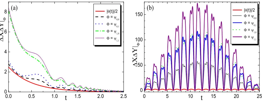
In order to display the deviation from the lower bound we depict in figure 2-4 the uncertainty for backgrounds corresponding to the solutions of the EP-equation displayed in figure 1. As expected from our analytical expressions in (4.16) and previous results, the smallest uncertainties are observed for the smaller quantum numbers.
0.0 0.5 1.0 1.5 2.0 2.5
0 2 4 6
8 |(t)|/2
=
=
=
=
X
Y
|
t (a)
0 5 10 15 20 25
0 50 100 150
|(t)|/2
=
=
=
=
X
Y
|
[image:14.595.89.506.383.546.2]t (b)
Figure 2: Uncertainties ∆X∆Y|ψn,m−n versus the generalized lower bound (a) for background
fields θ(t) = αe−γt and Ω(t) = βeγt and (b) for background fields θ(t) = αsin(γt) and Ω(t) =
βsin(γt/2). In both panels the constants are α= 5, β= 2,γ = 2, m= =τ =ω = 1, κ= 1/4 andµ= 5/3.
4.2 The generalized uncertainty relation for coherent states
0.0 0.2 0.4 0.6 0.8 1.0 1.2 1.4 0
20 40 60
| (t)|/2
=
=
=
=
P
x
P
y
|
t
(a)
0 5 10 15 20 25
0 30 60
90 | (t)|/2
=
=
=
=
P
x
P
y
|
[image:15.595.86.507.83.249.2]t (b)
Figure 3: Uncertainties ∆Px∆Py|ψ
n,m−n versus the generalized lower bound (a) for background
fields θ(t) = αe−γt and Ω(t) = βeγt and (b) for background fields θ(t) = αsin(γt) and Ω(t) =
βsin(γt/2). In both panels the constants are α= 5, β= 2,γ = 2, m= =τ =ω = 1, κ= 1/4 andµ= 5/3.
0.0 0.5 1.0 1.5 2.0 2.5
1 2 3 4 5 6 7
1/2+(t) (t)/8
=
=
=
=
X
P
x
|
t (a)
0 5 10 15 20 25
0 20 40 60 80 100 120
|1/2+(t) (t)/8|
=
=
=
=
X
P
x
|
t (b)
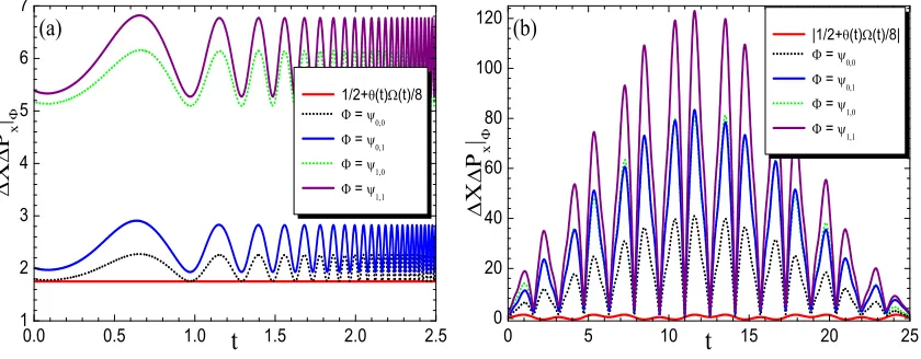
Figure 4: Uncertainties ∆X∆Px|ψn,m−n versus the generalized lower bound (a) for background
fields θ(t) = αe−γt and Ω(t) = βeγt and (b) for background fields θ(t) = αsin(γt) and Ω(t) =
βsin(γt/2). In both panels the constants are α= 5, β= 2,γ = 2, m= =τ =ω = 1, κ= 1/4 andµ= 5/3.
Glauber [31], who also coined the term coherent states. Since some of properties are very specific to the harmonic oscillator several types and generalizations of coherent states have been proposed thereafter to accommodate different types of situations, see for instance [32] for a review on the developments up to 2001. Fo instance, so-called Klauder [33, 34] and Gazeau-Klauder [35] cherent states, for which the quantum classical correspondence was recently investigated in [36, 37], are extremely useful.
[image:15.595.87.507.335.499.2]of Glauber coherent states [31]. Defining therefore the coherent states by means of the time-dependent displacement operatorD(α, t) as
|α, t :=D(α, t)|0,0 , with D(α, t) :=eαaˆ†(t)−α∗ˆa(t), (4.19)
it is immediately verified that they constitute eigenstates of the annihilation operatorˆa(t), i.e. ˆa(t)|α, t =α|α, t . Using the matrix elements for the expectation values with respect to the eigenfunction (4.1)-(4.8), we compute the expectation values with respect to the Glauber coherent states
α, t|x|α, t = −√ σImα, α, t|x2|α, t = σ2 1
2+ Im
2α , (4.20)
α, t|y|α, t = −√ σReα, α, t|y2|α, t = σ2 1
2+ Re
2α , (4.21)
α, t|px|α, t =√ Reα
σ −
˙
σImα
a , α, t|p
2
x|α, t = 2
1
σ2 + ˙
σ2
a2 + α, t|px|α, t 2,
α, t|py|α, t =−√ Imα
σ +
˙
σReα
a , α, t|p
2
y|α, t = 2
1
σ2 + ˙
σ2
a2 + α, t|py|α, t 2,
such that
∆x|2|α,t = ∆y|2|α,t = σ2
2 , ∆px|
2
|α,t = ∆py|2|α,t = 2
1
σ2 + ˙
σ2
a2 . (4.22)
Notice that the uncertainties are the same as those computed with respect to the ground stateψ0,0. Likewise we compute
∆X|2|α,t = ∆Y|
2
|α,t = ∆X|
2
ψ0,0, ∆Px|
2
|α,t = ∆Py|
2
|α,t = ∆Px|
2
ψ0,0, (4.23)
such that the uncertainty relations are identical to those in (4.16)-(4.18) withψ0,0 replaced
by |α, t . The crucial difference is of course that ψ0,0 is annihilated by a(t), whereas|α, t constitutes an eigenstate forˆa(t).
Having creation and annihilation operators at our disposal we can use standard tech-niques from quantum optics to construct squeezed states [38] and improve on the uncer-tainties obtained so far. Employing for this purpose the so-called squeezing operatorS(β, t)
by defining
|α, β, t :=S(β, t)D(α, t)|0,0 , with S(β, t) :=eβ2[ˆa2(t)−ˆa†2(t)], (4.24)
we may compute the relevant matrix elements for these states, not reported here. Using those we may subsequently deduce the uncertainties for the auxiliary variables to
∆x|2|α,β,t = ∆y|2|α,−β,t = 2σ2eβcoshβ, (4.25)
∆px|2|α,β,t = ∆py|2|α,−β,t = 2
1
σ2e
−β+σ˙2 a2e
and for our noncommutative variables to
∆X|2|α,β,t = ∆Y|
2
|α,−β,t = 2 σ2eβ+ θ2(t)
4 2 1
σ2e
β+ σ˙2 a2e
−β coshβ+θ(t)
4 (1−e 2β),
∆Px|2|α,β,t = ∆Py|2|α,−β,t = 2
1
σ2e
−β+σ˙2 a2e
β+Ω2(t)
4 2 σ
2e−β coshβ+Ω(t)
4 (1−e 2β).
As expected these expressions reduce to (4.22) and (4.23) whenβ →0.
We can now use the freedom to choose the functionβ(t) to minimize the uncertainties further. For instance, it is easily found that the uncertainty ∆x∆px||α,β,t is minimal for β(t) = βmin(t) = 1/2 ln a a2+ 8σ2σ˙2−a2 /(4σ2σ˙2) . Thus taking this value we
should find∆x∆px||α,βmin,t < ∆x∆px||α,t , which is indeed confirmed in figure 5, where
we observe that squeezing leads to a considerable reduction in the uncertainties.
0.0 0.2 0.4 0.6 0.8 1.0 1.2
0.50 0.55 0.60 0.65
= = | , t >
= |0,0,1.1,0.1>
= |0,0,1.1,0.5>
= |0,0,1.1,0.75>
= | ,
min
, t >
x p x | t (a)
0 1 2 3 4
0 1 2 3 4 5
= = |, t>
[image:17.595.85.505.266.433.2]= |0,0,1.1,0.1> = |0,0,1.1,0.5> = |0,0,1.1,0.75> = |, min , t> x p x | t (b)
Figure 5: Uncertainties with respect to Glauber coherent states versus squeezed Glauber coherent states and Gaussian Klauder coherent states for the auxiliary variablesx, px, ∆x∆px||α,t versus
∆x∆px||α,β,t versus ∆x∆px||GK> (a) for background fields θ(t) = αe−γt and Ω(t) = βeγt and
(b) for background fieldsθ(t) =αsin(γt)and Ω(t) =βsin(γt/2). In both panels the constants are
α= 5,β= 2,γ= 2,m= =τ =ω= 1, κ= 1/4and µ= 5/3.
The minimization for the uncertainties involving our noncommutative variables is less obvious. Due to the complexity of the expressions we can not perform this task for generic β(t), but only for specific instances in time. For instance, we find numerically the minimum for∆X∆Px||α,β,t=4 atβ =−1.88203. Indeed, as seen in figure 6 panel (a), at t= 4this
value leads to a reduction in the uncertainties when compared to∆X∆Px||α,t=4 .
However, for different values of time the uncertainties have grown considerably. It appears that the squeezing works only well for momentum-coordinate uncertainties as for instance ∆X ∆Y||α,β,t is always minimal at β(t) = 0, such that the squeezing does not lead to any reduction in these uncertainties. Figure 6 panel (b) exhibits these findings.
Let us next compare our findings with the uncertainties computed with respect to Gaussian Klauder coherent states defined as [39, 40, 41]
|GK =|n, m0, φ0, s := 1
N(m0) ∞
m=0
exp −(m−m0)
2
4s2 e
0 2 4 6 8 10 0
25 50 75 100
= = | , t>
= | , = -1.88 , t>
= | , = -0.4 , t>
= |1/2+(t) (t)/8|
X
P
x
|
t
(a)
0 2 4 6 8 10
0 200 400 600
= = | , t>
= | , = -1.88 , t>
= | , = -0.4 , t>
= |(t)/2|
X
Y
|
t
[image:18.595.88.506.83.248.2](b)
Figure 6: Uncertainties with respect to Glauber coherent states versus squeezed Glauber coherent
states for the noncommutative variablesX, Y, Px for background fieldsθ(t) =αsin(γt)andΩ(t) =
βsin(γt/2). In both panels the constants are α= 5, β= 2,γ = 2, m= =τ =ω = 1, κ= 1/4 andµ= 5/3.
with normalization factor N(m0) := ∞m=0exp −(m−m0)2/(2s2) , initial phase factor
φ0 and Gaussian standard deviation s. Using the matrix elements (4.1)-(4.8) we readily
compute the expectation values with respect to these states
GK|x|GK = − √
N(m0)σsin(φ0+α01)S1(m0), (4.28)
GK|y|GK = − √
N(m0)σcos(φ0+α01)S1(m0), (4.29)
GK|px|GK =
√
N(m0) 1
σ cos(φ0+α01)−
˙
σ
asin(φ0+α01) S1(m0), (4.30)
GK|py|GK = − √
N(m0) 1
σ sin(φ0+α01) +
˙
σ
acos(φ0+α01) S1(m0), (4.31)
and
GK|x2, y2|GK = σ 2
2N(m0) S2(n+ 1, m0)∓
√
2 cos(2φ0+α02)S3(m0) , (4.32)
GK|p2x, p2y|GK = 2N(m0)
1
σ2 + ˙
σ2
a2 S2(n+ 1, m0) (4.33)
±√2 1
σ2 − ˙
σ2
a2 cos(2φ0+α02)−2 ˙
σ
aσsin(2φ0+α02) S3(m0) ,
GK|xpy, ypx|GK =
2N(m0)
√
2 σσ˙
a sin(2φ0+α02)−cos(2φ0+α02) S3(m0) (4.34)
We abbreviatedG(m, m0) := exp −(m−m0)2/(4s2) and the sums
S1(y) : = ∞
k=0
√
k+ 1G(k, y)G(k+ 1, y), (4.35)
S2(x, y) : = ∞
k=0
(k+x)G2(k, y), (4.36)
S3(y) : = ∞
k=0
µ(k, k+ 2)G(k, y)G(k+ 2, y). (4.37)
One could make some approximations here for the sums by replacing them with Gaussian integrals, as for instance in [40, 42]. However, these sums converge very fast with only some of the initial terms taken into account and therefore it suffices here for our purposes to present numerical values. When the Gaussian enveloping function is very sharp we notice that the main contribution simply results from the center of the Gaussian. For instance, for s= 0.1, we compute S1(0)< 10−10, S2(n,0) =n, S3(0)< 10−10 and N(0) = 1, such that
∆o|2ψ0,0 = ∆o|
2
|α,t = ∆o|
2
|GK foro=x, y, px, py. (4.38)
This behaviour is clearly observable in figure 5. For a broader Gaussian enveloping function other modes start to contribute. For instance, for s = 0.5 we compute S1(0) = 0.3774, S2(0,0) = 0.1360, S2(1,0) = 1.2717, S3(0) = 0.0184 and N(0) = 1.1357 and for
s= 0.75we find S1(0) = 0.7998, S2(0,0) = 1.9092,S2(1,0) = 0.4693,S3(0) = 0.1897 and
N(0) = 1.4400. For these values the uncertainties for the auxiliary variables are depicted in figure 5 for two different types of background fields. We observe that depending on the instance of time the uncertainties might be lowered or increased.
When comparing with the uncertainties for the squeezed coherent states it appears that optimal minimum is dependent on the type of background field. We observe in figure 5 that for sinusoidal background fields the squeezed Glauber coherent states lead to minimal uncertainties which can not be undercut when using Gaussian Klauder coherent states instead, whereas for exponential backgrounds Gaussian Klauder coherent states allow for a further minimization.
5. Conclusions
explicit and to allow also for numerical studies thereafter, we have included here a detailed discussion of some solutions.
Our explicit solutions then allow for a analysis of the generalized uncertainty relations for which the lower bounds become time-dependent functions. Since our invariants are ex-pressed in terms of time-dependent creation and annihilation operators, standard Glauber coherent states were constructed by means of the displacement operator in a straightfor-ward manner. We found that the uncertainties for these states are identical to those of the ground state annihilated bya(t). By constructing the so-called squeezing operator we demonstrated that these uncertainties can be further minimized for momentum-coordinate uncertainties, where the absolute lower bound was only be reached for certain instances in time. For coordinate-coordinate uncertainties the minimal uncertainties were already reached by the Glauber coherent states and squeezing does not lead to any further im-provement. We compared these findings with an analysis for so-called Gaussian Klauder coherent states. A major difference towards the forgoing computations is that the phase αn,ℓ(t) becomes a relevant quantity. While in the computation of expectation values for eigenstates the phase always cancels due to the sum in|GK it leads here to interferences. We observe that also for the Gaussian Klauder coherent states the uncertainties resulting from the computations for the ground state and the nonsqueezed Glauber coherent state can be undercut. The answer to the question which type of the coherent states is optimal appears to be background field dependent. The time-dependent lowest bounds are well respected for all investigated scenarios.
There remain a multitude of challenges. First of all it would be highly desirable to investigate models on different types of time-dependent backgrounds rather than (1.1), possibly even those leading to minimal length. As always the study of different types of models will complete and enrich the understanding. The interesting question in all these different types of scenarios is whether they still allow for explicit solvability, which is one of the main virtue of our investigations, or if one needs to resort to additional approximations.
Acknowledgments: SD is supported by a City University Research Fellowship. AF thanks Abdelhafid Bounames and Boubakeur Khantoul for discussions.
References
[1] S. Doplicher, K. Fredenhagen, and J. E. Roberts, The Quantum structure of space-time at the Planck scale and quantum field, Commun. Math. Phys.172, 187—220 (1995).
[2] D. Gross and P. Mende, String Theory Beyond the Planck Scale, Nucl. Phys.B303, 407 (1988).
[3] D. Amati, M. Ciafaloni, and G. Veneziano, Can Space-Time Be Probed Below the String Size?, Phys. Lett. B216, 41 (1989).
[4] N. Seiberg and E. Witten, String theory and noncommutative geometry, J. High Energy Phys.JHEP09, 032 (1999).
[6] C. Rovelli, Loop Quantum Gravity, Living Rev. Relativity 11, 5 (2008).
[7] A. Kempf, G. Mangano, and R. B. Mann, Hilbert space representation of the minimal length uncertainty relation, Phys. Rev.D52, 1108—1118 (1995).
[8] B. Bagchi and A. Fring, Minimal length in Quantum Mechanics and non-Hermitian Hamiltonian systems, Phys. Lett.A373, 4307—4310 (2009).
[9] A. Fring, L. Gouba, and B. Bagchi, Minimal areas from q-deformed oscillator algebras, J. Phys.A43, 425202 (2010).
[10] S. Dey, A. Fring, and L. Gouba, PT-symmetric noncommutative spaces with minimal volume uncertainty relations, J. Phys.A45, 385302 (2012).
[11] S. Dey and A. Fring, Squeezed coherent states for noncommutative spaces with minimal length uncertainty relations, Phys. Rev. D86, 064038 (2012).
[12] X. Calmet, M. Graesser, and S. D. H. Hsu, Minimum Length from Quantum Mechanics and Classical General Relativity, Phys. Rev. Lett.93(21), 211101 (2004).
[13] H. Lewis and W. Riesenfeld, An Exact quantum theory of the time dependent harmonic oscillator and of a charged particle time dependent electromagnetic field, J. Math. Phys.10, 1458—1473 (1969).
[14] C. Ferreira, P. Alencar, and J. Bassalo, Wave functions of a time-dependent harmonic oscillator in a static magnetic field, Phys. Rev. A66, 024103 (2002).
[15] M. Maamache, A. Bounames, and N. Ferkous, Comment on ’Wave functions of a time-dependent harmonic oscillator in a static magnetic field’, Phys. Rev. A73, 016101 (2006).
[16] I. A. Pedrosa, Canonical transformations and exact invariants for dissipative systems, J. Maths. Phys. 28, 2662—2664 (1987).
[17] V. Ermakov, Transformation of differential equations„ Univ. Izv. Kiev.20, 1—19 (1880).
[18] E. Pinney, The nonlinear differential equationy′′3
= 0, Proc. Amer. Math. Soc.1, 681(1) (1950).
[19] J. R. Choi and B. H. Kweon, Operator method for a nonconservative harmonic oscillator with and without singular perturbation, Int. J. Mod. Phys.B16, 4733—4742 (2002).
[20] A. K. Rajagopal and J. T. Marshall, New coherent states with applications to time-dependent systems, Phys. Rev. A26, 2977—2980 (1982).
[21] A. Hone, Exact discretization of the Ermakov-Pinney equation, Phys. Lett. A263, 347—354 (1999).
[22] R. M. Hawkins and J. E. Lidsey, Ermakov-Pinney equation in scalar field cosmologies, Phys. Rev. D 66, 023523 (2002).
[23] J. R. Choi, Exact Wave Functions of Time-Dependent Hamiltonian Systems Involving Quadratic, Inverse Quadratic, and (1/x)p+p(1/x)Terms, Int. J. Theor. Phys.42, 853—861 (2003).
[25] S. C. Mancas and H. C. Rosu, Integrable dissipative nonlinear second order differential equations via factorizations and Abel equations, Phys. Lett. A377, 1434—1438 (2013).
[26] S. C. Mancas and H. C. Rosu, Integrable Ermakov-Pinney equations with nonlinear Chiellini ’damping’, arXiv:1301.3567 [math-ph] .
[27] A. Chiellini, Sull’integrazione dell’equazione differenzialey′2 +Qy3
= 0, Bolletino dell’Unione Matematica Italiana 10, 301—307 (1931).
[28] P. Caldirola, Forze non conservative nella meccanica quantistica, Il Nuovo Cimento18, 393—400 (1941).
[29] E. Kanai, On the quantization of the dissipative systems, Prog. Theor. Phys.3, 440—442 (1948).
[30] E. Schrödinger, Übergang von der Mikro- zur Makromechanik, Naturwissenschaften14, 664—666 (1926).
[31] R. J. Glauber, Coherent and Incoherent States of the Radiation Field, Phys. Rev.131, 2766—2788 (1963).
[32] V. Dodonov, ‘Nonclassical’ states in quantum optics: a ‘squeezed’ review of the first 75 years, J. Opt. B: Quantum Semiclass. Opt.4, R1—R33 (2002).
[33] J. Klauder, Quantization without quantization, Annals Phys.237, 147—160 (1995).
[34] J. Klauder, Coherent states for the hydrogen atom, J. Phys.A29, L293—L298 (1996).
[35] J. Gazeau and J. Klauder, Coherent states for systems with discrete and continuous spectrum, J. Phys. A: Math. Gen.32, 123—132 (1999).
[36] J.-P. Antoine, J.-P. Gazeau, P. Monceau, J. R. Klauder, and K. A. Penson, Temporally stable coherent states for infinite well and Pöschl—Teller potentials, J. Math. Phys. 42, 2349—2387 (2001).
[37] S. Dey and A. Fring, Bohmian quantum trajectories from coherent states, Phys. Rev. A88, 022116 (2013).
[38] R. Loudon and P. Knight, Squeezed Light, Journal of Modern Optics34, 709—759 (1987).
[39] R. F. Fox, Generalized coherent states, Phys. Rev. A59, 3241—3255 (1999).
[40] R. F. Fox and M. H. Choi, Generalized coherent states and quantum-classical correspondence, Phys. Rev. A61, 032107 (2000).
[41] J. R. Choi, Gaussian Klauder coherent states of general time-dependent harmonic oscillator, Phys. Lett. A325, 1—8 (2004).