Numerical methods for changing type systems

(1)

methods for changing type systems. Working paper. arXiv.org, Ithica, NY.

,

This version is available at https://strathprints.strath.ac.uk/61487/

Strathprints is designed to allow users to access the research output of the University of Strathclyde. Unless otherwise explicitly stated on the manuscript, Copyright © and Moral Rights for the papers on this site are retained by the individual authors and/or other copyright owners. Please check the manuscript for details of any other licences that may have been applied. You may not engage in further distribution of the material for any profitmaking activities or any commercial gain. You may freely distribute both the url (https://strathprints.strath.ac.uk/) and the content of this paper for research or private study, educational, or not-for-profit purposes without prior permission or charge.

Any correspondence concerning this service should be sent to the Strathprints administrator:

[email protected]

(2)

Sebastian Franz

∗

Sascha Trostorff

†

Marcus Waurick

‡

November 9, 2016

Abstract

In this note we develop a numerical method for partial differential equations with changing type. Our method is based on a unified solution theory found by Rainer Picard for several linear equations from mathematical physics. Parallel to the solu-tion theory already developed, we frame our numerical method in a discontinuous Galerkin approach in space-time with certain exponentially weighted spaces.

AMS subject classification (2010): 65J08, 65J10, 65M12, 65M60

Key words: evolutionary equations, changing type system, discontinuous Galerkin, space-time approach

Acknowledgements

M.W. carried out this work with financial support of the EPSRC frant EP/L018802/2: “Mathematical foundations of metamaterials: homogenisation, dissipation and operator theory”. This is gratefully acknowledged.

1 Introduction

Following the rationale presented in [9], most of the classical linear partial differential equations arising in mathematical physics share a common form, namely the form of an evolutionary problem. That is, we consider equations of the form

(∂tM0+M1+A)U =F, (1.1)

whereF is a given source term,∂t stands for the derivative with respect to time,M0, M1

are bounded linear operators on some Hilbert space H and A is an unbounded skew-selfadjoint operator in H. We are seeking for a unique solution U of the above equation.

∗_{Institut f¨}_{ur Numerische Mathematik, Technische Universit¨}_{at Dresden, 01062 Dresden, Germany.} e-mail: [email protected]

†_{Institut f¨}_{ur Analysis, Technische Universit¨}_{at Dresden, 01062 Dresden, Germany.} _e-mail: [email protected]

‡_{Department of Mathematical Sciences, University of Bath, Bath, UK. e-mail: [email protected]}

(3)

We remark here that we do not impose initial conditions, since we consider the whole real line as time horizon, and hence, we implicitly assume a vanishing initial value at “_−∞”. To illustrate the setting, we begin with presenting some examples.

Example 1.1. Let Ω _⊆ Rn _{an open non-empty set, where} _n _∈ N_{, but, typically} _n _∈

{1,2,3_}. We define the following two differential operators

∇0 :H01(Ω)⊆L2(Ω) →L2(Ω)n,

assigning each function u _∈ H1

0(Ω) its gradient, that is, the column-vector of its partial

derivatives in each coordinate direction. Moreover, we set

div := ₋(_∇0)∗ :D(div)⊆L2(Ω)n →L2(Ω),

which is nothing but the operator assigning each L2 _{vector-field its distributional}

diver-gence with maximal domain, that is,

D(div) ={v ∈L2(Ω)n :

n X

i=1

∂ivi ∈L2(Ω)}.

Since both the operators∇0 and div are closed and skew-adjoints of one another, we infer

that the operator

A:=

0 div

∇0 0

:D(_∇0)×D(div)⊆L2(Ω)×L2(Ω)n→L2(Ω)×L2(Ω)n

is skew-selfadjoint on the Hilbert space H = L2_(Ω) _×_L2_(Ω)n_{. Choosing} _M

0 = 1 and

M1 = 0 in (1.1), the corresponding evolutionary problem reads as

∂t+

0 div

∇0 0

u v

=

f g

.

If g = 0, this is nothing but the wave equation. Indeed, the second line then gives

∂tv =−∇0u, and hence, differentiating the first line with respect to time, we obtain

∂_t2u₋div_∇0u=∂ttu+ div∂tv =∂tf.

Note that div_∇0 = ∆D is the classical Dirichlet–Laplace operator on L2(Ω).

Choosing M0 =

1 0 0 0

and M1 =

0 0 0 1

in (1.1), the corresponding problem reads as

∂t

1 0 0 0

+

0 0 0 1

+

0 div

∇0 0

u v

=

f g

.

Setting again g = 0, the latter gives the heat equation. Indeed, the second line reads

v =_−∇0u and hence the first line yields

(4)

Finally, choosingM0 = 0 andM1 = 1 in (1.1), we get

1 +

0 div

∇0 0

u v

=

f g

,

which in the case g = 0 gives the elliptic equation

u₋div_∇0u=f.

Remark 1.2. We note that we can treat the case of homogeneous Neumann boundary

conditions in the same way. The only difference is that we define∇ as the distributional gradient onH1_{(Ω) and div}

0 :=−(∇)∗. Replacing now∇0 by∇and div by div0 yields the

same hyperbolic, parabolic and elliptic type problem above, but now with homogeneous Neumann boundary conditions.

Example 1.1 shows that evolutionary problems cover all three classical types of partial differential equations, elliptic, parabolic and hyperbolic. However, also problems of mixed type are covered as the next example shows.

Example 1.3. Recall the setting of Example 1.1. We decompose Ω into three measurable,

disjoint sets Ωell,Ωpar and Ωhyp and set M0 =

χΩhyp∪Ωpar 0

0 χΩhyp

as well as M1 =

χΩell 0

0 χΩpar∪Ωell

. The resulting evolutionary problem then is of mixed type. More

precisely, on Ωell we get an equation of elliptic type, on Ωpar the equations becomes

parabolic while on Ωhyp the problem is hyperbolic.

Remark 1.4. The interested reader might wonder that there is not imposed any

trans-mission condition on the unknown quantities along the interfaces of Ωell,Ωpar and Ωhyp.

However, this can be implemented automatically by being in the domain of the corre-sponding operator sum, as can be seen, for instance, in [23, Remark 3.2], see also [13, An illustrative Example]. Another example of a mixeed tyoe problem in contral theory can be found in [12, Remark 6.2]

In [9], the well-posedness of problems of the form (1.1) has been addressed. In fact, it was shown that these probolems also cover the classical Maxwell’s equations, the equations of linearized elasticity or a general class of coupled phenomena, see, for instance, [7, 8, 11]. All these problems are indeed well-posed (see Section 2 for the precise statement). The purpose of the present article is to provide numerical methods for such problems. In this article, for the applications to follow, we will focus, however, on problems of mixed type of the form sketched in Example 1.3. Moreover, as the spatial discretisation has to be developed for each problem separately, anyway, in this work, we will put an emphasize on the time-discretisation. Furthermore, we want to stress that the null-space of M0 in

(1.1) might be infinite-dimensional. Hence, we seek to develop a numerical scheme, which in particular allows for the treatment of a certain class of (partial) differential-algebraic

(5)

For the numerical treatment of the time derivatives we use a discontinuous Galerkin (dG) method, see also Section 3. The first dG-method was published in 1973 on neutron transport [15]. Later the methodology was developed further for classical hyperbolic, parabolic and elliptic problems, see also the survey article [4] and the book [16]. Note that there is a strong connection between dG-methods and Runge-Kutta (collocation) methods, see [2] for parabolic problems.

In Section 2, for convenience, we will recall some essentials for evolutionary equations. In particular, we recall the solution theory of problems of the type of equation (1.1). We will introduce a semi-dicretised version, Equation (3.1), of equation (1.1) at the beginning of Section 3. We will also provide a solution theory for this semi-discretised variant with general underlying (spatial) Hilbert spaceH(Proposition 3.1). The remainder of Section 3 is devoted to estimate difference of the exact solution of (1.1) and the approximate solution of (3.1): In Subsection 3.1, we bound the error by solely in terms of the interpolation error, which will eventually be estimated in Subsection 3.2. As our prime example, we address the full space-time discretisation of Example 1.3 and derive corresponding error estimates. We verify our theoretical findings in Section 5 by means of a 1 + 1- and a 1 + 2-dimensional numerical example. This article is attached an appendix (Section 6), where, for the convenience of the reader, we recall some well-known results on the Gauß– Radau quadrature rule including the fact that the choice of Gauß–Radau points depends continuously on the weighting function. We will need some implications of the fact just mentioned in our a-priori analysis in Subsection 3.1.

2 The setting of evolutionary problems

In this section we briefly recall the well-posedness result stated in [9]. For doing so, we need to specify the functional analytic setting. Throughout, letH be a real Hilbert space.

Definition. Letρ >0 and define the space

Hρ(R;H) :={f :R→H : f meas., Z

R

|f(t)_|2_Hexp(₋2ρt) dt <_∞},

where we as usual identify functions which are equal almost everywhere. The space

Hρ(R;H) is a Hilbert space endowed with the natural inner product given by

hf, g_iρ:= Z

R

hf(t), g(t)_iHexp(−2ρt) dt (f, g∈Hρ(R;H)).

Moreover, we define ∂t to be the closure of the operator

∂t :Cc∞(R;H)⊆Hρ(R;H)→Hρ(R;H) :ϕ 7→ϕ′,

where byC∞

c (R;H) we denote the space of infinitely differentiableH-valued functions on

R _{with compact support. We denote the domain of}_∂k

(6)

Within the setting introduced, we can formulate the well-posedness for evolutionary equa-tions of the form (1.1).

Theorem 2.1 ( [9, Solution Theory]). Let M0, M1 :H→H be bounded linear operators,

M0 selfadjoint and A :D(A)⊆H →H skew-selfadjoint. Moreover, assume that there is

some ρ0 >0 such that

∃γ >0_∀ρ_≥ρ0, x∈H :h(ρM0 +M1)x, xiH ≥γhx, xiH.

Then, for each ρ≥ ρ0 and each F ∈ Hρ(R;H) there exists a unique U ∈ Hρ(R;H) such

that

(∂tM0+M1+A)U =F, (2.1)

where the closure is taken in Hρ(R;H). Moreover, the following continuity estimate holds

|U_|ρ≤

1

γ|F|ρ.

If F _∈Hk

ρ(R;H) for k ∈N, then so is U and we can omit the closure bar in (2.1).

Remark 2.2.

(a) Note that the positive definiteness condition in the latter theorem especially implies

hM0x, xiH ≥0 for each x∈H.

(b) We remark thatH1

ρ(R;H)֒→Cρ(R;H) by a variant of the Sobolev embedding

theo-rem [10, Lemma 3.1.59] or [5, Lemma 5.2]. Here,

Cρ(R;H) := {f :R→H : f cont., sup t∈R|

f(t)_|exp(₋ρt)<_∞}.

(c) If F ∈H1

ρ(R;H) then U ∈Hρ1(R;H) and hence

AU =F ₋∂tM0U −M1U ∈Hρ(R;H),

which yields that U(t)∈ D(A) for almost every t∈ R_{. If even} _{F, U} _∈_H2

ρ(R;H) the

latter givesAU _∈H1

ρ(R;H) and hence, using the Sobolev embedding result (see part

(b)), U _∈Cρ(R;D(A)).

(d) The original result in [9] treat a general class of time-translation invariant coeffi-cients. We refer to [13, 22] for non-autonomous variants as well as to [19, 20] for non-autonomous and/or non-linear versions of Theorem 2.1.

(7)

3 Semi-discretisation in time

In this section, we discretise (1.1) with respect to time and do the a-priori analysis. We assume that A, M0, M1 satisfy the assumptions of Theorem 2.1. Let ρ≥ρ0 and fixT > 0

and consider the time interval [0, T] instead of the whole real line. We partition the time-interval [0, T] into subintervals Im = (tm−1, tm] of length τm for m ∈ {1,2, . . . , M} with

t0 = 0 and tM =T. Let q∈N. We define the space

Uτ _:= _{_u_∈_H

ρ(R;H) : ∀m∈ {1, . . . , M}:u|Im ∈ Pq(Im;H)},

where we denote by

Pq(Im;H) := lin{Im ∋t 7→tkζ ∈H;k ∈ {0, . . . , q}, ζ ∈H}

the space ofH-valued polynomials of degree at mostqdefined onIm. We endowPq(Im;H)

with the scalar product

hp, q_iρ,m := tm

Z

tm−1

hp(t), q(t)_iHexp(−2ρ(t−tm−1)) dt

turning the space _Pq(Im;H) into a Hilbert space.

The time integrals have to be evaluated numerically. We choose on each time interval Im

a right-sided weighted Gauß–Radau quadrature formula. To this end, denote by ωm i and

ˆ

tm

i , i∈ {0, . . . , q}, the weights and nodes of the weighted Gauß–Radau formula withq+ 1

nodes on the reference time interval Ib= (₋1,1], such that

Z

b

I

e−ρτm(t+1)_p₍_t_{) d}_t ₌

q X

i=0

ω_imp(ˆtm_i )

holds for all polynomials p of degree at most 2q. Note that the weights and nodes can always be numerically computed as shown for instance in [14, Chapter 4.6], see also the appendix (Section 6) for some basic facts on the Gauß–Radau quadrature. With the following standard transformation

Tm :Ib→Im, tˆ7→

tm−1+tm

2 +

τm

2 t,ˆ

we define by

Qm[v] :=

τm

2

q X

i=0

ω_imv(tm,i)

with the transformed Gauß–Radau points tm,i := Tm(ˆtim), i = {0, . . . , q}, a quadrature

formula on Im. Note that

Qm[p] = Z

Im

(8)

for all polynomials of degree at most 2q. Using

Qm[a, b]_ρ:=Qm[ha, biH]

instead of the scalar products _ha, b_iρ we employ the following discrete quadrature

for-mulation:

For givenF ∈ Uτ _and_x

0 ∈H, findU ∈ Uτ, such that for all Φ∈ Uτandm ∈ {1,2, . . . , M}

it holds

Qm[(∂tM0+M1+A)U,Φ]_ρ+hM0[[U]]xm0−1,Φ+m−1iH =Qm[F,Φ]_ρ. (3.1)

Here, we denote by

[[U]]x0

m−1 := (

U(tm−1+)−U(tm−1−), m∈ {2, . . . , M}

U(t0+)−x0, m= 1,

and by Φ+

m−1 := Φ(tm−1+).

Proposition 3.1. Let F _{∈ U}τ_{, x}

0 ∈H. Then there exists a unique solution of (3.1).

Proof. Let m ∈ {1, . . . , M} and recall that Pq(Im;H) is a Hilbert space with the

afore-mentioned scalar product. We note that

∂t :Pq(Im;H)→ Pq(Im;H) : p7→p′

and

δm−1 :Pq(Im;H)→R: p7→p(tm−1+)

are bounded linear operators. Consequently, the mapping

Pq(Im;H)→R:p7→ hx, δm−1piH

is linear and bounded for each x ∈ H and thus, by the Riesz representation theorem, there is a unique Ψ(x)_{∈ P}q(Im;H) such that

hΨ(x), p_iρ,m =hx, δm−1piH.

Moreover, the mapping Ψ :H → Pq(Im;H) is linear and bounded, since

|Ψ(x)_|2_ρ,m =_hΨ(x),Ψ(x)_iρ,m =hx, δm−1Ψ(x)iH ≤ |x|Hkδm−1k|Ψ(x)|ρ,m (x∈H).

We now prove that for each g ∈ Pq(Im;H) there is a unique u∈ Pq(Im;D(A)) such that

(9)

For doing so, we first compute using integration by parts

h∂tM0v, viρ,m

= 1

2h∂tM0v, viρ,m+ 1

2hv, ∂tM0viρ,m

= 1

2h∂tM0v, viρ,m+ 1 2

tm

Z

tm−1

hv(t), M0v′(t)iHexp(−2ρ(t−tm−1)) dt

= 1

2h∂tM0v, viρ,m− 1 2

tm

Z

tm−1

hM0v′(t), v(t)iH exp(−2ρ(t−tm−1)) dt

+ρ

tm

Z

tm−1

hM0v(t), v(t)iH exp(−2ρ(t−tm−1)) dt+

1

2hM0v(tm), v(tm)iHexp(−2ρτm)

− 1

2hM0v(tm−1), v(tm−1)iH

≥ρ_hM0v, viρ,m−

1

2hΨM0δm−1v, viρ,m

for eachv _{∈ P}q(Im;H). Next, from A∗ =−A it follows hAx, xiH = 0 for each x∈ D(A).

Therefore, for all u∈ Pq(Im;D(A)) we get

h(∂tM0+M1+A)u+ ΨM0δm−1u, uiρ,m

=_h∂tM0u, uiρ,m+hM1u, uiρ,m+hΨM0δm−1u, uiρ,m

≥ h(ρM0 +M1)u, uiρ,m+

1

2hΨM0δm−1u, uiρ,m

≥γ_hu, u_iρ,m,

where we have used

hΨM0δm−1u, uiρ,m =hM0u(tm−1+), u(tm−1)iH ≥0.

In particular, bothB := (∂tM0+M1) + ΨM0δm−1 andB+A are strictly positive definite.

Moreover, since B is bounded, B∗ _{is strictly positive definite, as well. Hence, from}

(B+A)∗ =B∗₋A

we read off that (B+A)∗ _{is strictly positive definite as well. Thus, for each}_g _{∈ P}

q(Im;H)

there is a unique u_{∈ P}q(Im;D(A)) =D(A+B) such that

(∂tM0+M1+A)u+ ΨM0δm−1u=g (3.2)

Thus, we are in the position to define a solution for (3.1) by induction on m. For this, we put U(t0−) := x0. Next, assume we have solved (3.1) for U on Im−1 for some m ∈

(10)

that (3.2) holds for g = F|Im −ΨM0U(tm−1−). We put U|Im := u. The thus defined

function U solves (3.1): We observe

h(∂tM0+M1+A)U,Φiρ,m+hΨM0δm−1U,Φiρ,m

=hF −ΨM0U(tm−1−),Φiρ,m =hF,Φiρ,m+hΨM0U(tm−1−),Φiρ,m,

by definition for all Φ_{∈ U}τ _and _m_{∈ {}₁_{, . . . , M}_}_{. The latter is the same as saying}

h(∂tM0+M1+A)U,Φiρ,m+hM0U(tm−1+),Φ(tm−1+)iH

=_hF,Φ_iρ,m+hM0U(tm−1−),Φ(tm−1+)iH.

But, since the quadrature is exact for polynomials up to degree 2q, the latter equation in turn is equivalent to

Qm[(∂tM0+M1+A)U,Φ]_ρ+hM0[[U]]xm0−1,Φ+m−1iH =Qm[F,Φ]_ρ,

which yields existence of U. Uniqueness follows from the uniqueness of usatisfying (3.2).

3.1 On some a-priori error estimates in time

After having proved the unique solvability of (3.1), we address the error estimates in the following. In our analysis we will use the discretised norms

|||v|||2Q,ρ,m:=Qm[v, v]ρ and |||v||| 2 Q,ρ :=

M X

m=1

Qm[v, v]ρe−2ρtm−1

as approximations of_|||v_|||2_ρ,m := R_I_m_|v(t)_|2

Hexp(−2ρ(t−tm−1)) dt and |v|2ρ. Note that for

v ∈ Uτ _{the approximation is exact.}

Let us start by defining an interpolation operator into _Uτ _{and define by} _ϕ

m,i with i ∈

{0, . . . , q_} the associated Lagrange basis functions to the nodes tm,i. Then we obtain for

a functionv ∈C([0, T], H) by

(P v)(0) =v(0), (P v)_I

m(t) =

q X

i=0

v(tm,i)ϕm,i(t), m∈ {1, . . . , M}, (3.3)

an interpolation operator in time.

In the analysis to follow, we will consider the problem (2.1). In particular, we emphasize that we assume that

the hypotheses of Theorem 2.1 are in effect.

Furthermore, we fix a right-hand side

(11)

Thus, by Theorem 2.1 (and Remark 2.2(c)) there exists a unique solution

U _∈H_ρ2(R_;_H_{) with (}_∂_t_M₀₊_M₁₊_A₎_U ₌_F. _(3.4)

Also, by Remark 2.2(c), we obtain F _∈ Cρ(R;H) and U ∈ Cρ(R;D(A)). Moreover, we

set

Uτ _{∈ U}τ _{to satisfy (3.1) for the right-hand side} _{P F} _{∈ U}τ _and _x

0 := U(0+).

We consider the following splitting

Uτ ₋_U ₌_ξ₋_η, _where _ξ ₌_Uτ ₋_{P U} _{∈ U}τ _and _η ₌_U ₋_{P U.}

Note that for almost every t _∈[0, T] we have that

(∂tM0+M1+A)U(t) =F(t)

and thus,

h(∂tM0+M1+A)U(t),Φ(t)iH =hF(t),Φ(t)iH

for each Φ_{∈ U}τ _{and almost every} _t_∈_[0_{, T}_{], which gives}

Qm[(∂tM0+M1+A)U,Φ]_ρ+hM0[[U]]mx0−1,Φ+m−1iH =Qm[F,Φ]_ρ=Qm[P F,Φ]_ρ,

where we have used M0[[U]]xm0−1 = M0[[U]]U(0+)m−1 = 0, due to the continuity of U and

Qm[F,Φ]ρ = Qm[P F,Φ]ρ, since the P F is interpolates at the Gauß–Radau points used

in the quadrature. Hence, U solves the same semi-discretised problem as Uτ_{. Thus, we}

obtain with χ_{∈ U}τ _{as test function the} _{error equation}

Qm[(∂tM0+M1+A)ξ, χ]_ρ+hM0[[ξ]]0m−1, χ+m−1iH

=Qm[(∂tM0+M1 +A)η, χ]_ρ+hM0[[η]]0m−1, χ+m−1iH. (3.5)

For the special case χ=ξ (use A=₋A∗_{) we obtain}

Em

d :=Qm[(∂tM0+M1)ξ, ξ]ρ+hM0[[ξ]]0m−1, ξm+−1iH

=Qm[(∂tM0+M1+A)η, ξ]_ρ+hM0[[η]]0m−1, ξm+−1iH =:Eim (3.6)

for all m ∈ {1, . . . , M}, where the subscripts d and i should remind of discretisation and interpolation, respectively.

Lemma 3.2. For all m _{∈ {}1, . . . , M_}, we have

E_dm ≥ 1

2

hM0ξm−, ξm−iHe−2ρτm− hM0ξm−−1, ξm−−1iH +hM0[[ξ]]m0 −1,[[ξ]]0m−1iH

+γ|||ξ|||2Q,ρ,m,

where ξ−

(12)

Proof. Let m ∈ {1, . . . , M}. Since ξ is a (piece-wise) polynomial of order q in time, we obtain

Qm[∂tM0ξ, ξ]_ρ=h∂tM0ξ, ξiρ,m

= 1 2

Z

Im

e−2ρ(t−tm−1)_∂

thM0ξ, ξiHdt

= 1 2

hM0ξ−m, ξm−iHe−2ρτm − hM0ξm+−1, ξm+−1iH+ρhM0ξ, ξiρ,m.

Further, we compute

hM0[[ξ]]0m−1, ξm+−1iH =

1 2

hM0ξm+−1, ξm+−1iH − hM0ξm−−1, ξm−−1iH +hM0[[ξ]]m0−1,[[ξ]]0m−1iH

.

Therefore, we have

E_dm =Qm[(∂tM0+M1)ξ, ξ]ρ+hM0[[ξ]]0m−1, ξm+−1iH

= 1 2

hM0ξm−, ξ−miHe−2ρτm− hM0ξm−−1, ξm−−1iH +hM0[[ξ]]m0−1,[[ξ]]0m−1iH

+_h(ρM0+M1)ξ, ξiρ,m.

Together with

h(ρM0+M1)ξ, ξiρ,m ≥γ|||ξ|||2_ρ,m =γ|||ξ|||2_Q,ρ,m

the lemma is proved.

In order to analyse Em

i we introduce another interpolation operator, that enables us to

estimate the time derivative of the interpolation error with a higher order. This operator utilises tm,−1 := tm−1 in addition totm,i, i∈ {0, . . . , q} as interpolation points. Denoting

the associated Lagrange basis functions by ψm,i, i ∈ {−1,0, . . . , q}, this interpolation

operator is given by

(P vb )_I

m(t) :=

q X

i=−1

v(tm,i)ψm,i(t), m∈ {1, . . . , M}. (3.7)

Note the Pb maps to functions that are continuous in time (recall that tm,q = tm) while

the image of P is allowed to be discontinuous at the time mesh points.

Lemma 3.3. For m_{∈ {}1, . . . , M_} and ψ _{∈ U}τ_{, we have}

Qm[∂tM0η, ψ]_ρ+hM0[[η]]0m−1, ψm+−1iH =Qm h

∂tM0(U −P Ub ), ψ i

ρ+R(U, ψ),

where

|R(U, ψ)_{| ≤}Cατm|M0η+m−1|2H +β|||ψ||| 2 Q,ρ,m

(13)

Proof. With U being continuous in time, we only have to consider the discrete part. Using the exactness of the quadrature rule for polynomials of degree 2q, we obtain for

m_{∈ {}1, . . . , M_}

Qm[∂tM0P U, ψ]ρ+hM0[[P U]]xm0−1, ψm+−1iH

| {z }

=:a

=h∂tM0P U, ψiρ,m+a

=−hM0P U, ∂tψiρ,m+ 2ρhM0P U, ψiρ,m+he−2ρ(t−tm−1)M0P U, ψiH tm

tm−1

| {z }

=:b

+a

=₋Qm[M0P U, ∂tψ]ρ+ 2ρhM0P U, ψiρ,m+a+b

=−Qm h

M0P U, ∂b tψ i

ρ+ 2ρhM0P U, ψiρ,m+a+b

=−hM0P U, ∂b tψiρ,m+ 2ρhM0P U, ψiρ,m+a+b

=h∂tM0P U, ψb iρ,m+ 2ρ(hM0P U, ψiρ,m− hM0P U, ψb iρ,m)

+a+b_{− h}e−2ρ(t−tm−1)_M

0P U, ψb iH tm

tm−1

| {z }

=:c

.

Using (P U)−_m₋₁ = (P Ub )+_m₋₁ (m _≥ 2), (P Ub )+₀ = U(0+) = x0 and (P U)−m = (P Ub )−m

(m≥1), we have

a+b₋c= 0.

Furthermore, it holds

2ρ(hM0P U, ψiρ,m− hM0P U, ψb iρ,m) = 2ρhM0(P −Pb)U, ψiρ,m

= 2ρhM0((P −Pb)U)(t+m−1)χ, ψiρ,m

= 2ρhM0(P U−U)(tm+−1)χ, ψiρ,m =:R(U, ψ),

where χ _{∈ P}q+1(Im) with χ(tm−1) = 1 and χ(tm,i) = 0, i ∈ {0, . . . , q}. By Corollary 6.5

for K =T (note that 0< τm =|Im| ≤T), we obtain Z

Im

|χ(t)_|2e−2ρ(t−tm−1)_dx _≤_Cτ

m

for some C _≥0. Thus, we get

|R(U, ψ)| ≤2ρM0(P U −U)(t+m−1)χ

ρ,m|||ψ|||ρ,m

= 2ρ _|M0(P U −U)(t+m−1)|H|||χ|||_ρ,m|||ψ|||_ρ,m

≤C2(2ρ)2ατm|M0(P U −U)(t+m−1)|2+β|||ψ||| 2 Q,ρ,m,

where αβ = 1/4. Combining above transformations we are done.

Lemma 3.4. For all m _{∈ {}1, . . . , M_}, we have for all ψ _{∈ U}τ

(14)

Proof. These equalities follow from the fact thatη(tm,i) = P U(tm,i)−U(tm,i) = 0 for each

i_{∈ {}0, . . . , q_} and M1, A are purely spatial operators.

Combining the previous lemmas gives a first result.

Theorem 3.5. There exists a C _≥0 depending on T, ρ and γ, only, such that

hM0ξM−, ξM−iH + e2ρT|||ξ|||2Q,ρ ≤Ce2ρT

∂tM0(U −P Ub ) 2 Q,ρ

+T max

1≤m≤M

|M0ηm+−1|2He−2ρtm−1

=:g(U).

Proof. Combining Lemmas 3.2 to 3.4 for ψ =ξ we have for some C _≥1 depending on T

and ρ only

|E_dm| ≥ 1

2

hM0ξm−, ξm−iHe−2ρτm− hM0ξ−m−1, ξm−−1iH +hM0[[ξ]]m0 −1,[[ξ]]0m−1iH

+γ|||ξ|||2Q,ρ,m,

|E_im_{| ≤}Cα ∂tM0(U −P Ub ) 2

Q,ρ,m+τm|M0η + m−1|2H

+ 2β_|||ξ_|||2_Q,ρ,m.

Summing with weights e−2ρtm−1 _for _m∈ {₁_{, . . . , M}} _{we obtain}

M X

m=1

e−2ρtm−1

|E_dm_{| ≥} 1

2

hM0ξM−, ξM−iHe−2ρtM − hM0ξ0−, ξ0−iH

+1 2

M X

m=1

e−2ρtm−1_h_M

0[[ξ]]0m−1,[[ξ]]m0 −1iH +γ|||ξ|||2Q,ρ,

≥ 1

2hM0ξ

−

M, ξM−iHe−2ρT +γ|||ξ|||2_Q,ρ,

byξ₀− = 0 and neglecting the positive jump-contributions, and

M X

m=1

e−2ρtm−1

|E_im_{| ≤}Cα ∂tM0(U−P Ub ) 2

Q,ρ+T 1≤maxm≤M{|M0η +

m−1|2He−2ρtm−1}

+ 2β|||ξ|||2Q,ρ.

Thus for β < γ/2 the result is proved upon the equality Em

i =Edm.

Remark 3.6. Letm_{∈ {}1, . . . , M_}. Note that the estimate in Theorem 3.5 remains valid,

if one respectively replacesT bytm, ξM− byξm− as well as the |||·|||Q,ρ by|||·χI˜|||Q,ρ with χI˜

being the characteristic function of ˜I =Sm_k=1Ik.

(15)

2.1]. For the upcoming result and the corresponding proof, we recall for polynomials

a, b_{∈ P}q(0,1;H)

ha, b_iρ= Z 1

0 h

a(t), b(t)_iHe−2ρtdt

and the corresponding integration by parts formula

ha′, b_iρ =−ha, b′iρ+ 2ρha, biρ+ e−2ρtha, biH 1

0. (3.8)

Lemma 3.7. Let ti, wi, i∈ {0, . . . , q} be the points and weights of the right-sided

Gauß-Radau quadrature rule of order q on (0,1] with weighting function t7→e−2ρt_.

Let p _{∈ P}q(0,1;H) and p˜ the Lagrange interpolant w.r.t. (ti)i∈{0,...,q} of ϕ: (0,1] ∋ t 7→

p(t)/t. Then

hp′,p˜_iρ+hp(0),p˜(0)iH ≥

1

2 |p(1)|

2

He−2ρ+hp,˜ p˜iρ+ρhp,p˜iρ

≥ 1₂ |p(1)_|2_He−2ρ+_hp, p_iρ+ρhp, piρ.

Proof. Definev _{∈ P}q−1((0,1);H) by v(t) = (p(t)−p(0))/t and Λ∈ Pq[0,1] by

Λ(ti) =

1

ti

, i∈ {0, . . . , q}.

Then

p(t) = p(0) +tv(t) and p˜(t) = v(t) +p(0)Λ(t).

Thus,

hp′,p˜_iρ=hv+ mv′, v+p(0)Λiρ

=hv, viρ+hv,mv′iρ+hv, p(0)Λiρ+hv′, p(0)mΛiρ,

where we denote by m the multiplication-with-the-argument, that is, (mf)(t) := tf(t). With (3.8) we obtain for the second term

hv′,mviρ=

1 2 e

−2ρ_|_v₍₁₎_|2

H + 2ρhmv, viρ− hv, viρ

.

From mv′_Λ _{∈ P}

2q−1 and mΛ′Λ ∈ P2q together with the exactness of the quadrature rule

it follows that

hv′, p(0)mΛ_iρ= q X

i=0

wihv′(ti), p(0)iHti

1

ti

=_hv′, p(0)_iρ

= 2ρ_hv, p(0)_iρ+ e−2ρhv(1), p(0)iH − hv(0), p(0)iH,

and in the same way

(16)

We have thus this far

hp′,p˜_iρ=

1 2 e

−2ρ

|v(1)_|2_H +_hv, v_iρ+ 2ρhmv, viρ+

+_hv, p(0)Λ_iρ+ 2ρhv, p(0)iρ+ e−2ρhv(1), p(0)iH − hv(0), p(0)iH.

Using v(1) = p(1)₋p(0) and_hp(0),p˜(0)_iH =hp(0), v(0)iH + Λ(0)|p(0)|2H we obtain

hp′,p˜_iρ+hp(0),p˜(0)iH =

1 2 e

−2ρ

|p(1)_|2_H +_hv, v_iρ+ 2ρhmv, viρ

+hv, p(0)Λiρ+ 2ρhv, p(0)iρ+|p(0)|2H

Λ(0)− e

−2ρ

2

.

Next, (3.9) yields

Λ(0) = 2ρhΛ,1iρ+ e−2ρ− hΛ′,mΛiρ

= 2ρhΛ,1iρ−ρhΛ,mΛiρ+

1 2 e

−2ρ₊_h_Λ_,_Λ_i ρ

and hence

hp′,p˜iρ+hp(0),p˜(0)iH =

1 2 e

−2ρ_|_p₍₁₎_|2

H +hv, viρ+ 2ρhmv, viρ

+hv, p(0)Λiρ+ 2ρhv, p(0)iρ+|p(0)|2H

ρhΛ,2−mΛiρ+

1

2hΛ,Λiρ

With 1

2hv, viρ+hv, p(0)Λiρ+ 1 2|p(0)|

2

HhΛ,Λiρ=

1

2hv+p(0)Λ, v+p(0)Λiρ= 1 2hp,˜ p˜iρ it follows

hp′_,_p_˜_i

ρ+hp(0),p˜(0)iH =

1 2 e

−2ρ_|_p₍₁₎_|2

H +hp,˜ p˜iρ

+ρ _hmv, v_iρ+ 2hv, p(0)iρ+|p(0)|2HhΛ,2−mΛiρ.

Finally,

hmv, viρ+ 2hv, p(0)iρ+|p(0)|2hΛ,1iρ = q X

i=0

wi

1

ti

(t2_i|v(ti)|2H + 2tihv(ti), p(0)iH +|p(0)|2H)

=

q X

i=0

wi

1

ti|

p(ti)|2H

=

q X

i=0

wihp(ti),p˜(ti)iH

(17)

gives

hp′,p˜_iρ+hp(0),p˜(0)iH =

1 2 e

−2ρ

|p(1)_|2_H +_hp,˜ p˜_iρ+ρ hp,p˜iρ+|p(0)|2HhΛ,1−mΛiρ.

Using _hΛ,1₋mΛ_iρ≥ 0, which we provide in Lemma 3.8, the first result is proved. The

second one follows upon using the exactness of the quadrature rule and t−_i 1 >1.

Lemma 3.8. Let Λ _{∈ P}q[0,1] such that Λ(ti) = _t1_i for i ∈ {0, . . . , q}, where ti is chosen

as in Lemma 3.7. Then

hΛ,1−mΛiρ≥0,

where (mΛ)(t) :=tΛ(t).

Proof. We rewrite the scalar product as a quadrature error:

hΛ,1₋mΛ_iρ= q X

i=0

wi

1

ti − Z 1

0

e−2ρttΛ2(t) dt =Q[f]₋I[f]

for f given by f(t) = tΛ2₍_t_{), where} _Q_[_g_{] =} Pq

i=0wig(ti) and I[g] = R1

0 g for suitable g.

There exists a constant α_∈R _{and a polynomial}_w₀ _{∈ P}_q₋₁_[0_,_{1], such that}

Λ(t) =αtq+w0(t) which implies f(t) =α2t2q+1+w1(t),

where w1 ∈ P2q[0,1]. Thus, setting g(t) = t2q+1, we have that

hΛ,1−mΛiρ=α2(Q[g]−I[g]),

due to the exactness of the quadrature rule for polynomials of degree 2q. Let Πw_{∈ P}2q[0,1] be an Hermite-interpolant of a given function w satisfying

Πw(ti) = w(ti), i∈ {0, . . . , q},

(Πw)′(ti) = w′(ti), i∈ {0, . . . , q−1}.

Then it follows

Q[g] =

q X

i=0

wit2q+1i = q X

i=0

wi(Πg)(t2q+1i ) =Q[Πg] =I[Πg].

Using that for each t_∈[0,1] there is ζ _∈(0,1) such that

(Πg)(t)−g(t) =−g

(2q+1)₍_ζ₎

(2q+ 1)!(t−1)

q−1 Y

i=0

(t−ti)2 = (1−t) q−1 Y

i=0

(t−ti)2

see, for instance, [18, Section 2.1.5], we infer that

hΛ,1−mΛiρ =α2I[Πg−g]

=α2

Z 1

0

e−2ρt

q−1 Y

i=0

(t−ti)2 !

(18)

Now we are able to improve Theorem 3.5 following [1, Corollary 2.1] and [21].

Theorem 3.9. There exists C _≥0 depending on T, q, _kM0k, kM1k, γ, and ρ such that

sup

t∈[0,T]h

M0ξ(t), ξ(t)iH ≤Cg(U),

with g(U) defined as in Theorem 3.5.

Proof. For the discrete error ξ =Uτ ₋_{P U} _{∈ U}τ _{we define}_ϕ _by

ϕ_|Im =P

t_7→ τm t₋tm−1

ξ(t)

(m_{∈ {}1, . . . , M_}).

Then for all m_{∈ {}1, . . . , M_} and i_{∈ {}0, . . . , q_}we have

hM0ϕ(tm,i), ϕ(tm,i)iH =

τm

tm,i−tm−1h

M0ξ(tm,i), ξ(tm,i)iH ≥ hM0ξ(tm,i), ξ(tm,i)iH

and by Lemma 3.7 (apply the lemma to the functions p=√M0ξ and ˜p=√M0ϕ rescaled

on [0,1])

Qm[∂tM0ξ,2ϕ]ρ+hM0ξm+−1,2ϕ+m−1iH ≥

1

τm

Qm[M0ϕ, ϕ]ρ≥

1

τm

Qm[M0ξ, ξ]ρ.

By the equivalence of norms on _Pq([0,1]), there existsK1 ≥0 depending onq only, such

that

sup

t∈[0,1]|

p(t)| ≤K1 1 Z

0

|p(t)|dt (p∈ Pq([0,1])).

Consequently, we obtain for all m∈ {1, . . . , M}

sup

t∈Im

hM0ξ(t), ξ(t)iH ≤

K1

τm

e2ρτm_Q

m[M0ξ, ξ]ρ≤

K τm

Qm[M0ξ, ξ]ρ

where K :=K1e2ρT ≥ max m∈{1,...,M}{e

2ρτm} ≥_K

1. Moreover, we have

Qm[Aξ,2ϕ]ρ =

τm

2

q X

i=0

ωm

i hAξ(tm,i),2ϕ(tm,i)iH

= τm 2

q X

i=0

ω_im 2τm tm,i−tm−1h

Aξ(tm,i), ξ(tm,i)iH = 0

uponA =₋A∗_{. Together, it follows for all} _m_{∈ {}₁_{, . . . , M}_}

sup

t∈Im

hM0ξ(t), ξ(t)iH

≤KQm[(∂tM0+M1+A)ξ,2ϕ]ρ+hM0ξm+−1,2ϕ+m−1iH −Qm[M1ξ,2ϕ]ρ

=K

Qm[(∂tM0+M1+A)ξ,2ϕ]_ρ+hM0[[ξ]]0m−1,2ϕ+m−1iH

+_hM0ξm−−1,2ϕ+m−1iH −Qm[M1ξ,2ϕ]_ρ

(19)

Using the error equation (3.5) with χ= 2ϕ (recall η=U −P U), we obtain

sup

t∈Im

hM0ξ(t), ξ(t)iH ≤K

Qm[(∂tM0+M1+A)η,2ϕ]_ρ+hM0[[η]]m−1,2ϕ+m−1iH

+_hM0ξm−−1,2ϕ+m−1iH −Qm[M1ξ,2ϕ]_ρ

.

Using Lemma 3.3, Lemma 3.4 with ψ = 2ϕ and Theorem 3.5, we estimate further with some C1 ≥1 depending onq, T, and ρ such that

sup

t∈Im

hM0ξ(t), ξ(t)iH ≤K

Qm h

∂tM0(U −P Ub ),2ϕ i

ρ+R(U,2ϕ)

+hM0ξm−−1,2ϕ+m−1iH −Qm[M1ξ,2ϕ]ρ

≤C1α1

∂tM0(U−P Ub ) 2

Q,ρ,m+|M0(P U−U)(t + m−1)|2

+C1α2hM0ξm−−1, ξm−−1iH +C1α1kM1k2|||ξ|||2_Q,ρ,m

+ 3β1Qm[2ϕ,2ϕ]_ρ+β2h2M0ϕ+m−1,2ϕ+m−1iH,

where αiβi = 1₄,i∈ {1,2}and we used that

hM0u, vi=h p

M0u, p

M0vi ≤ hM0u, uihM0v, vi

for allu, v ∈H, by the non-negativity and selfadjointness ofM0. Using Theorem 3.5 (and

Remark 3.6), we, thus, get

sup

t∈Im

hM0ξ(t), ξ(t)iH ≤C(α1+α2)g(U) + 3β1Qm[2ϕ,2ϕ]ρ+β2h2M0ϕ+m−1,2ϕ+m−1iH (3.10)

for some C ≥1 depending on q, T, ρ, and kM1k, where g(U) is defined in Theorem 3.5.

Next, by Corollary 6.6, we find c >0 depending onρ and T only such that

τm

tm,i−tm−1 ≤

τm

tm,0−tm−1 ≤

1

c (m∈ {1, . . . , M}).

Hence, for all m _{∈ {}1, . . . , M_},

Qm[2ϕ,2ϕ]_ρ≤LQm[ξ, ξ]_ρ= (4/c)|||ξ|||2_Q,ρ,m

and h2M0ϕ+m−1,2ϕ+m−1iH ≤(4/c) sup t∈Im

hM0ξ(t), ξ(t)iH.

Next, we chooseβ2 = (4/c)1₂. Thus, appealing to (3.10), we obtain for allm∈ {1, . . . , M}

1 2tsup∈Im

hM0ξ(t), ξ(t)iH = sup t∈Im

hM0ξ(t), ξ(t)iH −

1 2tsup∈Im

hM0ξ(t), ξ(t)iH

≤C(α1+α2)g(U) + 3β1(4/c)|||ξ|||2Q,ρ,m,

(20)

3.2 Estimating the interpolation error in time

In the previous section we showed that the discrete error is bounded in terms of the interpolation errors. We finalize the error estimates in time in this section focussing on the interpolation error. The aim and, thus, main theorem of this section is Theorem 3.13, where we estimate the difference between the exact solution U of (3.4) and the solution

Uτ _{of the quadrature formulation (3.1) with right-hand side}_{P F} _{and initial value} _U_(0+).

We use the same notation as in the previous section. In addition, we set τ := max{τm :

m _{∈ {}1, . . . , M_}}. Moreover, shall further assume that the hypotheses of Theorem 2.1 are in effect.

Lemma 3.10. There existsC _≥0depending onqandT such that for allV _∈Hq+3

ρ (R;H)

∂t(V −P Vb )

Q,ρ ≤Cτ q+1

|∂_tq+3V_|ρ.

Proof. First we note thatHq+3

ρ (R;H)֒→Cρq+2(R;H) by the Sobolev-embedding theorem.

By the definition of _|||·|||_Q,ρ we have that

∂t(V −P Vb ) 2 Q,ρ = M X m=1 Qm h

|∂t(V −P Vb )|2He−2ρt i = M X m=1 τm 2 q X i=0

ω_im_|(∂t(V −P Vb ))(tm,i)|2He−2ρtm,i.

Using the standard result from interpolation theory

sup

t∈Im

|(v₋P vb )′(t)_{| ≤}Cτ_mq+1 sup

t∈Im

|v(q+2)(t)_|,

for all v ∈Wq+2,∞₍₀_{, T}_{) we obtain}

∂t(V −P Vb ) 2

Q,ρ≤C 2 M X m=1 τm 2 τ 2(q+1) m q X i=0

ωm_i sup

t∈Im

|∂p+2_t V(t)_|2_He−2ρtm,i

≤C2τ2(q+1) sup

t∈[0,T]|

∂_tp+2V(t)_|2_H.

For the next two lemmas, we recall the standard result from interpolation theory

sup

t∈Im

|(v−P v)(t)| ≤Cτ_mq+1 sup

t∈Im

|v(q+1)(t)|, (3.11)

for all v _∈Wq+1,∞₍₀_{, T}_{), see, for instance, [18, Section 2.1.4].}

Lemma 3.11. There existsC _≥0depending onqandT such that for allV _∈Hq+2

ρ (R;H)

(21)

Proof. We obtain

|(V ₋P V)(t+

m−1)|H ≤ sup t∈Im

|(V ₋P V)(t)_|H

≤Cτmq+1sup t∈Im

|∂tq+1V(t)|H.

The claim follows from the Sobolev-embedding theorem.

With the previous lemmas we can already estimate g(U). Now let us estimate the final term needed to estimate the errorU −Uτ_.

Lemma 3.12. There existsC ≥0depending onT andqsuch that for allU ∈Hq+2

ρ (R;H)

sup

t∈[0,T]h

M0(U−P U)(t),(U −P U)(t)iH

≤Cτ2(q+1)|∂tq+2U|2ρ.

Proof. Using the Cauchy–Schwarz and Young inequality we derive

sup

t∈[0,T]h

M0(U −P U)(t),(U−P U)(t)iH

≤ 1

2 t∈sup[0,T]|

M0(U −P U)(t)|2H + sup t∈[0,T]|

(U −P U)(t)|2 H

!

.

Using (3.11) with v =M0U and v =U we obtain

sup

t∈[0,T]|

M0(U−P U)(t)|H ≤Cτq+1 sup t∈[0,T]|

∂tq+1M0U(t)|H,

sup

t∈[0,T]|

(U₋P U)(t)_|H ≤Cτq+1 sup t∈[0,T]|

∂_tq+1U(t)_|H.

Combining these results the claim follows from the Sobolev-embedding theorem.

Combining the previous lemmas, Theorem 3.5 and Theorem 3.9, we can bound the discrete error in time.

Theorem 3.13. Assume that U ∈ Hq+3

ρ (R;H). Then there exists C ≥ 0 depending on

kM0k, kM1k, ρ, T, γ, q such that

sup

t∈[0,T]h

M0(U −Uτ)(t),(U −Uτ)(t)iH +|||U−Uτ|||2_Q,ρ≤Cτ2(q+1)|∂tq+3U|2ρ.

Proof. By Lemma 3.10 and Lemma 3.11 applied to V =M0U we have that

g(U)_≤C1τ2(q+1)|∂tq+3U|2ρ

for some C1 ≥ 0. We note that |||U −Uτ|||_Q,ρ ≤ |||η|||_Q,ρ+|||ξ|||_Q,ρ =|||ξ|||_Q,ρ and hence,

by Theorem 3.5 we obtain

(22)

Moreover,

hM0(U −Uτ)(t),(U−Uτ)(t)iH ≤2hM0η(t), η(t)iH + 2hM0ξ(t), ξ(t)iH

and thus, by Theorem 3.9 and Lemma 3.12 we infer

sup

t∈[0,T]h

M0(U −Uτ)(t),(U −Uτ)(t)iH ≤C(τ2(q+1)|∂tq+2U|2ρ+g(U))

for some C _≥0. Combining these estimates, the claim follows.

Remark 3.14. The above analysis holds for all evolutionary problems and gives error

bounds for the semi-discrete solution of order q+ 1, assuming enough regularity in time. For a fully discrete method, a spatial discretisation has to be defined too. This step, however, has to be done for each problem considered separately.

4 Full discretisation for Example 1.3

Let us assume a regular, quasi uniform and shape-regular triangulation Ωh of Ω into

triangular open cells σ with maximal cell diameter h. Moreover, we assume that the interfaces between Ωell, Ωpar and Ωhyp are polygonal such that the triangulation Ωh fits to

these interfaces.

As the whole article is mainly concerned with the correct time-discretization, in this section, we will employ the custom of the “generic constant” C _≥ 0 that may vary from line to line, which, however, depends on T, ρ, kM1k, kM0k, q, and γ and on k, the order

of the assumed spatial regularity, only. Then the fully discretised counterpart _Uτ

h toU is given by

Uhτ :={(uh, vh)∈ Uτ : uh|Im ∈ Pq(Im, V1(Ω)), vh|Im ∈ Pq(Im, V2(Ω)), m∈ {1, . . . , m}},

where the spatial spaces are

V1(Ω) :=

v ∈H₀1(Ω);∀σ : v|σ ∈ Pk(σ) ,

V2(Ω) :={w∈H(div,Ω);∀σ : w|σ ∈RTk−1(σ)}.

Here_Pk(σ) is the space of polynomials of degree up to k on the cell σ and RTk−1(σ) is a

the Raviart-Thomas-space, defined by

RTk−1(σ) = (Pk−1(σ))n+xPk−1(σ).

Note that

Pk−1(σ)⊂RTk−1(σ)⊂ Pk(σ),

div(RTk−1(σ))⊂ Pk−1(σ) and

RTk−1(σ)·n|∂σ⊂ Pk−1(∂σ).

Furthermore, if the mesh consists of quadrilateral or hexahedral cells, in above defini-tions and statements the polynomials spacePk(σ) can be replaced byQk(σ) including all

(23)

Remark 4.1(Solvability of the fully discrete system). We can apply the general existence theory that was also used in Proposition 3.1. More precisely, the positive definiteness still holds, since the triangulation fits to the interfaces and hence, the uniqueness of the system is warranted. However, since the problem is finite-dimensional, the uniqueness implies the existence of a solution of the fully discretised problem.

Let us come to the interpolation operator I = (I1, I2). For I1 : C(Ω) → V1 we use the

Scott–Zhang interpolant on each cell σ, see [17] for a precise definition, that is patched together continuously. Here local interpolation error estimates can be given using L2

-norms also in 3d, which is not possible for standard Lagrange interpolation. For I2 :

W →V2 with

W(σ) =q_∈(Ls(σ))n: divq _∈L2(σ) , s >2,

we also use the standard interpolator, defined via moments, see [3]. Note that in the following, in order to avoid a cluttered notation as much as possible, we will not ex-plicitly keep track on the number of components of the L2_{(Ω)- or} _Hk_{(Ω)-spaces under}

consideration, as it will be obvious from the context.

Standard local interpolation error estimates yield for all v _∈H1

0(Ω)∩Hr(Ω)

kv₋I1vk0,Ω ≤Chrkvkr,Ω,

k∇(v₋I1v)k0,Ω ≤Chr−1kvkr,Ω,

where 1≤r ≤k+ 1 and for all q∈Hs_{(Ω) such that div}_q_∈_Hs_(Ω)

kq₋I2qk0,Ω ≤Chskqks,Ω,

kdiv(q−I2q)k0,Ω ≤Chskdivqks,Ω,

where 1_≤s _≤k, see [3]. Let Uτ

h ∈ Uhτ be the solution of the fully discretised system and P IU ∈ Uhτ be the

interpolated solution of (1.1) for the operatorsM0, M1 given in Example 1.3 and Agiven

as in Example 1.1. Then we obtain analogously to the derivation of the errors of the semi-discretisation

sup

t∈[0,T]h

M0(P IU −Uhτ)(t),(P IU−Uhτ)(t)iH +|||P IU −Uhτ||| 2 Q,ρ

≤C ∂tM0(U −P IUb ) 2

Q,ρ+|||M1(U −P IU)||| 2

Q,ρ+|||A(U −P IU)||| 2 Q,ρ

+T max

1≤m≤M

|M0(P IU−IU)(t+m−1)|2He−2ρtm−1 !

, (4.1)

where we remark that in contrast to Theorem 3.5 the terms |||M1(U −P IU)|||2Q,ρ and

(24)

start with a term partcularly needed for the final convergence estimate in Theorem 4.7. Beforehand, let us introduce

kuk2

Q,ρ,k,D = M X

m=1

Qm

|u|2 k,D

e−2ρtm−1

where D⊆Ω is measurable.

Lemma 4.2. It holds for U = (u, v)_∈Hρ(R;Hk(Ω)×Hk(Ω))

|||U ₋P IU_|||_Q,ρ _≤Chk _ku_kQ,ρ,k,Ω+hkkvkQ,ρ,k,Ω,

Moreover, if U = (u, v)∈Hρ(R;D(A)) such that AU ∈Hρ(R;Hk(Ω)×Hk(Ω)), then

|||A(U ₋P IU)_|||_Q,ρ _≤Chk(_ku_kQ,ρ,k+1,Ω+kdivvkQ,ρ,k,Ω).

Proof. By the definition of Qm[·]ρ we have

|||U₋P IU_|||2_Q,ρ =_|||U ₋IU_|||2_Q,ρ

=

M X

m=1

QmkU −IUk20,Ω

e−2ρtm−1

=

M X

m=1

Qm

ku−I1uk20,Ω+kv−I2vk20,Ω

e−2ρtm−1

≤C

M X

m=1

Qm

h2(k+1)_|_u₍_·₎_|2

k+1,Ω+h2k|v(·)|2k,Ω

e−2ρtm−1

=C h2(k+1)_ku_k2_Q,ρ,k+1,Ω+h2k_kv_k2_Q,ρ,k,Ω.

Very similarly we have for the second norm

|||A(U ₋P IU)_|||2_Q,ρ =_|||A(U ₋IU)_|||2_Q,ρ

=

M X

m=1

Qmk∇(u−I1u)k0,Ω2 +kdiv(v−I2v)k20,Ω

e−2ρtm−1

≤C

M X

m=1

Qmh2k|u|k+1,Ω2 +h2k|divv|2k,Ω

e−2ρtm−1

=Ch2k _ku_k2_Q,ρ,k+1,Ω+_kdivv_k2_Q,ρ,k,Ω.

Lemma 4.3. It holds for U = (u, v)∈Hρ(R;Hk(Ω)×Hk(Ω))

|||M1(U−P IU)|||2_Q,ρ≤Ch2k(kukQ,ρ,k,Ω+kvkQ,ρ,k,Ω)2

(25)

Lemma 4.4. For U = (u, v)∈H1

ρ(R;Hk(Ω)×Hk(Ω))∩Hρq+2(R;L2(Ω)×L2(Ω)) we have

that

sup

t∈[0,T]h

M0(U −P IU)(t),(U −P IU)(t)iH

≤C h2k sup

t∈[0,T]

(_|u(t)_|k,Ω+|v(t)|k,Ω)2+τ2(q+1)|∂tq+2IU|ρ !

.

Proof. The operator M0 is selfadjoint and non-negative. Thus it follows that

hM0(U −P IU)(t),(U −P IU)(t)iL2_(Ω)

=_|pM0(U −P IU)(t)|2L2_(Ω)

≤2|pM0(U−IU)(t)|2L2_(Ω)+|

p

M0(IU −P IU)(t)|2L2_(Ω)

for each t _∈[0, T]. The second term can be estimated by

|pM0(IU −P IU)(t)|L22_(Ω) ≤Cτ2(q+1)|∂_tq+2IU|2_ρ

according to Lemma 3.12, while the first term can be estimated by

|pM0(U −IU)(t)|2L2_(Ω)≤Ch2k |u(t)|2_k,Ω+|v(t)|2_k,Ω

,

due to the boundedness of √M0. Hence, the assertion follows.

Lemma 4.5. For U = (u, v)_∈H1

ρ(R;Hk(Ω)×Hk(Ω))∩Hρq+3(R;L2(Ω)×L2(Ω)) we get

∂tM0(U−P IUb ) 2

Q,ρ ≤C h 2k₍_k_∂

tukQ,ρ,k,Ω+k∂tvkQ,ρ,k,Ω)2+τ2(q+1)|∂tq+3IU|ρ !

.

Proof. We have that

∂tM0(U −P IUb )

_Q,ρ ≤ |||∂tM0(U −IU)|||Q,ρ+

∂t(M0IU −P Mb 0IU) _Q,ρ

≤ |||M0(∂tU −I∂tU)|||Q,ρ+Cτq+1|∂ q+3 t IU|ρ,

by Lemma 3.10. For the first term we have by Lemma 4.2

|||M0(∂tU −I∂tU)|||2Q,ρ ≤Ch2k k∂tuk2Q,ρ,k,Ω+k∂tvk2Q,ρ,k,Ω

.

Lemma 4.6. It holds for U = (u, v)∈Hq+2

ρ (R;L2(Ω)×L2(Ω))

max

1≤m≤M

|M0(P IU −IU)(t+m−1)|L2_(Ω)e−ρtm−1 ≤Cτq+1|∂_tq+2IU|_ρ.

(26)

Lemma 4.2 to 4.6 give us all needed estimates for the final convergence result for Exam-ple 1.3.

Theorem 4.7. We assume for the solution U = (u, v) of Example 1.3 the regularity

U _∈H_ρ1(R_;_Hk_(Ω)_×_Hk_(Ω))_∩_H_ρq+3₍R_;_L2_(Ω)_×_L2_(Ω)) as well as

AU _∈Hρ(R;Hk(Ω)×Hk(Ω)).

Then we have for the error of the numerical solution by (3.1)

sup

t∈[0,T]h

M0(U −Uhτ)(t),(U −Uhτ)(t)iH +|||U−Uhτ||| 2

Q,ρ ≤C(τ

2(q+1)₊_{T h}2k₎_.

5 Numerical examples

In the following section we consider some examples to verify numerically our theoretical findings.

5.1 Changing type system – one space dimension

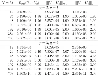
Let Ω = (₋π 2,

π 2)⊂R

1_{, Ω}

h = (−π₂,0) and Ωp = (0,π₂). The problem is given onR×Ω by

∂t

1 0 0 χh

+

0 0 0 χp

+

0 ∂x

∂x 0

u v

=

f g

(5.1a)

with u(t,₋π

2) = u(t, π

2) = 0, g = 0 and

f(t, x) =χR_≥₀(t)(2et−1−tχ₍₋π

2,0)(x)) cos(x). (5.1b)

The solution can be derived as

u(t, x) =χR_≥₀(t)(et−1) cos(x), v(t, x) =χR_≥₀(t)(et−1−tχ₍₋π

2,0)(x)) sin(x).

Note that a priori, we impose no transmission condition. However, as in [23, Remark 3.2], they can be derived for u satisfying (5.1) as

u(t,0+) =u(t,0₋), ∂xu(t,0+) = Z t

0

∂xu(s,0−)ds.

The solution up to a timeT = 1 is shown in Figure 1. For the numerical solution we use again T = 1, an equidistant mesh of M cells in time and an equidistant mesh of N cells in space. In order to resolve the boundary S = Ωh ∩Ωp ={0} we assume N to be even.

(27)

−π

2

0

π

2

0 0.5 1

0 1 2

x

t −π

2

0

π

2

0 0.5 1

0 2

[image:27.595.114.488.89.260.2]

x t

[image:27.595.91.495.230.687.2]

Figure 1: Solution u (left) and v (right) of problem (5.1)

Table 1: Convergence results for U ₋Uh of problem (5.1)

N =M Esup(U −Uh) |||U−Uh|||_Q,ρ |||U −Uh|||_ρ

p= 2, q= 1

8 8.727e-03 7.766e-04 1.855e-03 16 2.335e-03 1.90 1.939e-04 2.00 4.638e-04 2.00 32 6.039e-04 1.95 4.851e-05 2.00 1.160e-04 2.00 64 1.535e-04 1.98 1.213e-05 2.00 2.899e-05 2.00 128 3.871e-05 1.99 3.032e-06 2.00 7.248e-06 2.00 256 9.717e-06 1.99 7.580e-07 2.00 1.812e-06 2.00 512 2.434e-06 2.00 1.895e-07 2.00 4.530e-07 2.00

p= 3, q= 2

Defining

Esup(v) = sup t∈[0,T]h

M0v(t), v(t)iH !1/2

, E(v) = sup

t∈[0,T]h

M0v(t), v(t)iH +|||v|||2Q,ρ !1/2

we consider in Table 1 the convergence behaviour ofUhforN =M and polynomial degrees

q=p+ 1 = 2 andq =p+ 1 = 3. Note that we also show the norm |||U −Uh|||ρestimated

(28)

support our theoretical result in Theorem 4.7, that the error E is of order min{p, q+ 1}. For odd polynomial degreesp the component_|||U ₋Uh|||Q,ρ shows a convergence order of

one order higher, hinting at a superconvergence property.

[image:28.595.238.359.208.296.2]

In Table 2 the estimated convergence rates for all combinations of polynomial degrees

Table 2: Convergence rates for E(U−Uh) of problem (5.1) and several polynomial orders

p_\q 1 2 3 4 5 1 2 2 2 2 2 2 2 2 2 2 2 3 2 3 4 4 4 4 2 3 4 4 4 5 2 3 4 5 6

{p, q_{} ⊆ {}1, . . . ,5_}are given. Clearly the rates for even pfollow the predicted min_{p, q+ 1}, while for odd pthe rates are min{p+ 1, q+ 1}. Thus there might be dragons1_.

Let us modify problem (5.1), by taking Ω = ₋3π 2 ,

3π 2

, Ωh =

−3π 2 ,0

, Ωp =

0,3π 2

and right-hand sides only inL2_{. To be more precise, let}

f(t, x) =χR_≥₀(t)

−(2et₋t₋1)χ₍₋π

2,0)(x) cos(x) + e

t_χ

(π

2, 3π

2 )(x)−χ(0,

π

2)(x)

cos(x)+

χ(0,π)(x)−χ₍_π,3π

2 )(x)

,

g(t, x) =χR_≥

0(t)

χ(0,π)(x)x+χ₍_π,3π

2)(x)(2π−x)

−(et₋₁₎₍_χ

(π

2, 3π

2 )(x)−χ(0,

π

2)(x)) sin(x)

.

Figure 2 shows the right-hand sides f and g fort = 1. Again the exact solution can be found and is given by

u(t, x) =χR_≥₀(t)(et−1)(χ

(π

2, 3π

2)(x)−χ(− 3π

2,

π

2)(x)) cos(x),

v(t, x) =χR_≥₀(t)

−(et−t−1)χ₍₋3π

2,0)(x) sin(x) +χ(0,π)(x)x+χ(π, 3π

2 )(x)(2π−x)

.

Note that u and v are non-differentiable, but piece-wise smooth. Figure 3 shows the solutions for t _∈[0,1].

Note that a priori, we impose no transmission condition. However, as in [23, Remark 3.2], they can be derived for u satisfying (5.1) as

u(t,0+) =u(t,0−), ∂xu(t,0+) = Z t

0

∂xu(s,0−)ds.

(29)

−2π

2 −

π ₋π

2 0

π 2

π ₃π 2

−4 −2 0 2 4

x

t

[image:29.595.214.387.104.260.2]

f g

Figure 2: Right-hand sidesf and g of modified problem (5.1)

−2π

2 −π−π2

0 π2 π 3π

2

0 0_.5 1

−2 0 2

x

t −2π

2

−π−

π

2 0 π2

π 3π

2

0 0.5 1

0 2 4

x t

Figure 3: Solution u (left) and v (right) of the modified problem (5.1)

For the numerical solution we use T = 1, an equidistant mesh ofM cells in time and an equidistant mesh ofN cells in space, thus τ = 1/M and h= 1/N. In order to capture the jumps of f and g, and to resolve the boundary S = Ωh∩Ωp ={0}we use an equidistant

mesh in space with the number of cells N divisible by 6. Note that we can use ρ= 1 for the given solution u.

Defining

Esup(v)2 := sup t∈[0,T]h

M0v(t), v(t)iH, E(v)2 := sup t∈[0,T]h

M0v(t), v(t)iH +|||v|||2_Q,ρ

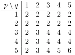
[image:29.595.118.480.320.476.2]

(30)

[image:30.595.138.460.134.388.2]

Table 3: Convergence results for U−Uh of problem modified (5.1)

N =M Esup(U −Uh) |||U−Uh|||Q,ρ |||U −Uh|||ρ

p= 2, q= 1

p= 3, q= 2

Table 4: Convergence rates for E(U −Uh) of the modified problem (5.1) and several

polynomial orders

p_\q 1 2 3 4 5 1 2 3 3 3 3 2 2 2 2 2 2 3 2 3 5 5 5 4 2 3 4 4 4 5 2 3 4 7 7

5.2 Changing type system – two space dimensions

This time we consider a problem with unknown solution. Let Ω = (0,1)2 _⊂ _R2_{, Ω} h = 1

4, 3 4

2

, Ωe= Ω\Ω¯h and Ωp =∅. The problem is given on (0, T)×Ω by

∂t

1 0 0 χh

+

0 0 0 χp

+

0 div

∇0 0

u v

=

f

0

, (5.2)

where

f(t, x) = 2 sin(πt)χR_<

1/2×R(x).

[image:30.595.238.358.459.543.2]

(31)

0 0.5 1 0

0.5

1

−0_.1 0

0_.1

0 0.5

1 0

0.5

1

−0_.1 0

0_.1

0 0.5

1 0

0.5

1

−0_.1 0

0_.1

0 0.5

1 0

0.5

1

−0_.1 0

0_.1

0 0.5

1 0

0.5

1

−0_.1 0

0_.1

0 0.5

1 0

0.5

1

−0_.1 0

[image:31.595.85.518.81.318.2]

0_.1

Figure 4: Solution u at times t = 5k/16 for k _{∈ {}1, . . . ,6_} (top left to bottom right) of problem (5.2) for T = 1.875

Table 5: Convergence results for ˜U ₋Uh of problem (5.2)

N =M Esup( ˜U −Uh)

U˜₋Uh

Q,ρ

U˜ ₋Uh

ρ

p= 2, q= 1

4 1.660e-02 8.121e-03 8.703e-03 8 5.595e-03 1.57 2.425e-03 1.74 2.781e-03 1.65 16 1.666e-03 1.75 7.445e-04 1.70 8.517e-04 1.71 32 5.260e-04 1.66 2.790e-04 1.42 3.012e-04 1.50 64 1.926e-04 1.45 1.300e-04 1.10 1.331e-04 1.18

p= 3, q= 2

4 4.895e-03 1.778e-03 2.028e-03 8 1.117e-03 2.13 5.510e-04 1.69 5.748e-04 1.82 16 4.015e-04 1.48 2.414e-04 1.19 2.419e-04 1.25 32 1.430e-04 1.49 1.175e-04 1.04 1.175e-04 1.04 64 5.245e-05 1.45 5.075e-05 1.21 5.072e-05 1.21

shows some snapshots of the componentuof the solutionU, approximated by a numerical simulation.

In order to investigate the error-behaviour upon refinement of the discretisation, we use a numerically computed reference solution ˜U instead of the real one U. For this we set

(32)

in time, and polynomial degrees p = 3 and q = 2. Thus u is approximated in space by piece-wise _Q3 elements,v by RT2-elements and both in time by P2-elements.

In Table 5 we see the results of our numerical simulation for two pairs of polynomial order. We observe, that the error rates are independent of the polynomial order and furthermore less than the optimal orders given in Theorem 4.7. The reason for this decrease in convergence order lies in the reduced regularity of the solution to this given problem. The interior boundaries where the type of the problem changes introduces corners, where it is very likely for singular solution components to arise.

References

[1] G. Akrivis and C. Makridakis. Galerkin time-stepping methods for nonlinear parabolic equations. ESAIM: M2AN, 38:261–289, 3 2004.

[2] G. Akrivis, C. Makridakis, and R. Nochetto. Galerkin and Runge–Kutta methods: unified formulation, a posteriori error estimates and nodal superconvergence. Nu-merische Mathematik, 118(3):429–456, 2011.

[3] F. Brezzi and M. Fortin. Mixed and hybrid finite element methods, volume 15 of

Springer Series in Computational Mathematics. Springer-Verlag, New York, 1991.

[4] B. Cockburn, G. E. Karniadakis, and C.-W. Shu. The Development of Discontinuous Galerkin Methods, pages 3–50. Springer Berlin Heidelberg, Berlin, Heidelberg, 2000.

[5] A. Kalauch, R. Picard, S. Siegmund, S. Trostorff, and M. Waurick. A Hilbert space perspective on ordinary differential equations with memory term. J. Dyn. Differ. Equations, 26(2):369–399, 2014.

[6] G. Lube Problemstellung. Orthogonale Polynome Online-manuscript: https: //lp.uni-goettingen.de/get/text/1275 and https://lp.uni-goettingen.de/ get/text/1276 available at 25/10/2016, Georg-August-University G¨ottingen, 2004.

[7] S. Mukhopadhyay, R. Picard, S. Trostorff, and M. Waurick. A note on a two-temperature model in linear thermoelasticity. Math. Mech. Solids, 2015.

[8] A. J. Mulholland, R. Picard, S. Trostorff, and M. Waurick. On well-posedness for some thermo-piezoelectric coupling models. Math. Methods Appl. Sci., 39(15):4375– 4384, 2016.

[9] R. Picard. A structural observation for linear material laws in classical mathematical physics. Math. Methods Appl. Sci., 32(14):1768–1803, 2009.

(33)

[11] R. Picard, S. Trostorff, and M. Waurick. On some models for elastic solids with micro-structure. ZAMM, Z. Angew. Math. Mech., 95(7):664–689, 2015.

[12] R. Picard, S. Trostorff, and M. Waurick. On a comprehensive Class of Linear Control Problems. IMA J. Math. Control Inf., 33(2):257–291, 2016.

[13] R. Picard, S. Trostorff, M. Waurick, and M. Wehowski. On Non-autonomous Evolu-tionary Problems. J. Evol. Equ., 13(4):751–776, 2013.

[14] W. H. Press, S. A. Teukolsky, W. T. Vetterling, and B. P. Flannery. Numerical Recipes 3rd Edition: The Art of Scientific Computing. Cambridge University Press, New York, NY, USA, 3 edition, 2007.

[15] W. H. Reed and T. R. Hill. Triangular mesh methods for the neutron transport equation. Submitted to American Nuclear Society Topical Meeting on Mathematical Models and Computational Techniques for Analysis of Nuclear Systems, Los Alamos Laboratory, 1973.

[16] B. Rivi`ere. Discontinuous Galerkin Methods for Solving Elliptic and Parabolic Equa-tions. Society for Industrial and Applied Mathematics, 2008.

[17] L. R. Scott and S. Zhang. Finite element interpolation of nonsmooth functions satisfying boundary conditions. Math. Comp., (54):483–493, 1990.

[18] J. Stoer, R. Bartels, W. Gautschi, R. Bulirsch, and C. Witzgall. Introduction to Numerical Analysis. Texts in Applied Mathematics. Springer New York, 2002.

[19] S. Trostorff. An alternative approach to well-posedness of a class of differential inclusions in Hilbert spaces. Nonlinear Anal., Theory Methods Appl., Ser. A, Theory Methods, 75(15):5851–5865, 2012.

[20] S. Trostorff and M. Wehowski. Well-posedness of non-autonomous evolutionary inclu-sions. Nonlinear Anal., Theory Methods Appl., Ser. A, Theory Methods, 101:47–65, 2014.

[21] M. Vlasak and H.-G. Roos. An optimal uniform a priori error estimate for an unsteady singularly perturbed problem. Int. J. Numer. Anal. Model., 11(1):24–33, 2014.

[22] M. Waurick. On non-autonomous integro-differential-algebraic evolutionary prob-lems. Math. Methods Appl. Sci., 38(4):665–676, 2015.

(34)

6 Appendix – On the Gauß–Radau Quadrature

In this appendix we shall gather some results on the right-sided Gauß–Radau quadrature, which are known in principle, but are included for the convenience of the reader. We adopted the rational given in [6]. For this, we introduce a set of weighting functions:

W :=_{w_∈L1(₋1,1) :w >0 a.e._}.

Note that the bilinear form

h·,·iw: (f, g)7→ Z 1

−1

f(x)g(x)w(x)dx

introduces a scalar product on its natural domain

D:={f _∈L1_loc(₋1,1);

Z

(−1,1)|

f(x)_|2w(x) dx <_∞}.

Furthermore, for allw_∈W we set ˜w: x_7→(1₋x)w(x). We observe ˜w_∈W. Throughout, let q ∈N_.

Definition. Letw_∈W. A pair (ω, r) = ((ωj)j∈{0,...,q},(rj)j∈{0,...,q})∈Rq+1×[−1,1]q+1 is

called(right-sided)w-Gauß–Radau quadrature (of orderq), if₋1_≤r0 ≤r1 ≤ · · · ≤rq = 1

and for all p∈ P2q(−1,1) we have Z 1

−1

p(x)w(x)dx=

q X

j=0

ωjp(rj).

Proposition 6.1. Let w _∈ W, (ω, r) a w-Gauß–Radau quadrature. Then the following

properties are satisfied:

1. the set _{rj;j ∈ {0, . . . , q}} consists of q+ 1 elements;

2. for all j _{∈ {}0, . . . , q_} we have 0< ωj ≤R₍₋_1,1)w(x)dx;

3. for all j ∈ {0, . . . , q} we have with Ij(x) :=Qk∈{0,...,q}\{j}

x−rk

rj−rk

ωj = Z 1

−1

Ij(x)w(x)dx;

4. if (ω(1)_{, r}(1)₎ _{is a} _w_{-Gauß-quadrature, then} ₍_{ω, r}_{) = (}_ω(1)_{, r}(1)₎_.

Proof. For the proof (1), we assume that Z := {rj;j ∈ {0, . . . , q}} has strictly less than

(35)

with the property pz(z) = 1 and pz = 0 onZ\ {z}. Thus, by exactness of the quadrature

and w >0 a.e., we obtain

0<

Z 1

−1

pz(x)2w(x)dx=

X

j∈{k;rk=z}

ωjpz(rj)2 =

X

j∈{k;rk=z} ωj.

Consequently, as p2 _{has degree at most 2}_q_{, we infer}

0<

Z 1

−1

p(x)2w(x)dx = X

j∈{0,...,q}

ωjp(rj)2

=X

z∈Z

X

j∈{k;rk=z}

ωjp(rj)2 = X

z∈Z

p(z)2 X

j∈{k;rk=z}

ωj = 0,

a contradiction.

Next, for (2), by (1), we observe that Ij(x) in (3) is well-defined for all j ∈ {0, . . . , q}.

Thus, for j _{∈ {}0, . . . , q_}, we obtain

0<

Z 1

−1

Ij(x)2w(x)dx=ωj.

Hence, we get for allj ∈ {0, . . . , q}

ωj ≤ X

ℓ∈{0,...,q}

ωℓ = Z 1

−1

w(x)dx.

The proof of (3) is obvious.

For the proof of (4), by the Gram–Schmidt orthonormalization procedure, we choose a polynomialpq ∈ Pq(−1,1) such thatpqis orthogonal toPq−1(−1,1) with respect toh·,·iw˜.

Letp∈ Pq−1(−1,1). Then the polynomial (1− ·)ppq has degree at most 2q. Thus, by the

choice of pq and the exactness of the quadrature, we obtain

0 = hp, pqiw˜

=

Z 1

−1

(1₋x)p(x)pq(x)w(x)dx

= X

j∈{0,...,q}

ωj(1−rj)p(rj)pq(rj)

= X

j∈{0,...,q−1}