City, University of London Institutional Repository
Citation
: Slingsby, A. and van Loon, E. (2013). Visual Analytics for Exploring Changes in
Biodiversity. Paper presented at the Workshop on Visualisation in Environmental Sciences
(EnvirVis), Jul 2013, Leipzig, Germany.
This is the unspecified version of the paper.
This version of the publication may differ from the final published
version.
Permanent repository link:
http://openaccess.city.ac.uk/2385/
Link to published version
:
Copyright and reuse:
City Research Online aims to make research
outputs of City, University of London available to a wider audience.
Copyright and Moral Rights remain with the author(s) and/or copyright
holders. URLs from City Research Online may be freely distributed and
linked to.
City Research Online:
http://openaccess.city.ac.uk/
[email protected]
Eurographics Conference on Visualization (EuroVis) (2013) M. Hlawitschka and T. Weinkauf (Editors)
Visual Analytics for Exploring Changes in Biodiversity
A. Slingsby1and E. van Loon2
1School of Informatics, City University London, UK 2IBED, University of Amsterdam, The Netherlands
Abstract
We report on ongoing work in which we are designing a visual interface to a large database of species observation data. Our design allows the data to be explored and visually summarised by space, time and species, helping assess the data’s suitability for helping answer questions about biodiversity. Key issues we are addressing include working with large datasets, dealing with varying spatial and temporal precisions and dealing with different qualities of data collection and sampling strategies. Our visual interface design is being informed by a set of research questions and a planned user-centred workshop.
Categories and Subject Descriptors(according to ACM CCS): H.5.2 [Information Interfaces and Presentation]: User Interfaces—User-centered design
1. Introduction
The importance of maintaining long-term ecological records has been long recognised [MBB∗10]. Since much of envi-ronment is now heavily influenced and managed by humans, monitoring biodiversity is increasingly important. Research questions generated in conservation biology [SAA∗09] of-ten require data that originate from different sources that dif-fer in extent, observation properties and attributes. There has been rapid increase in availability of such data.
The Netherlands has an extensive network for collect-ing data on spatial and temporal distributions of flora and fauna from a variety of organisations, but not in a consis-tent form. The recently-established National Database of Flora and Fauna (NDFF) has collated these in
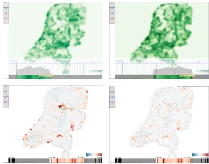
semantically-Figure 1: Observation footprint map (left; blue footprint outlines) and density estimation map (right), indicating the extents and numbers of observations at the mouse cursor.
consistent way. Over the past few decades, severalde jure
(Table 1 in [VvRS∗12] and [JSRB06]) andde facto (Dar-win Core and Access to Biological Collections Data) stan-dards have emerged and are widely supported. The NDFF is comparable with Darwin Core with the additional ad-vantage that it has not only syntactically but also seman-tically integrates datasets of different origins [VvRS∗12]. It contains 40 million observations of 7000 species of mammals, birds, reptiles, amphibians, fish, invertebrates, plants and fungi [VvRS∗12]. It offers good potential for studying species distributions and changes in biodiversity over space and time. Geographical and temporal visualisa-tion techniques are widely used for exploring observavisualisa-tion data [SWI∗09], species distributions and species distribu-tion models [FLF∗11] that use vegetation and other data to help improve the precision of such mapping [SP03]. How-ever, significant sampling and bias issues exist in the data due to the diversity of observations included.
[image:2.612.73.287.580.649.2]provid-A. Slingsby & E. van Loon / Visual Analytics for Exploring Changes in Biodiversity
ing graphical interactive interfaces to raw observation data over long timescales with variation in spatial and temporal precision, different survey types, different abundance mea-sures and large data sizes. We use visual analytics to study these and other issues (e.g. [Bow00]) related to data qual-ity and suitabilqual-ity for studying biodiversqual-ity. We describe and justify our design decisions, discuss shortcomings that we are addressing and outline our plans for assessing how ef-fective these techniques are for answering research questions from a group of ecologists.
2. Research questions
Biodiversity and conservation programmes require effec-tive communication between scientists and resource man-agers [CVC12]. This involves a good understanding of the strengths and weaknesses of available data by all parties. Answers to simple questions concerning data availability, occurrence of species-groups over space and time, need to be readily available. Examples of such questions include:
• What is the coverage in space and time of observations on a given species group?
• Has key-species X been observed in region A?
• Is there a temporal trend in abundance of species Y?
• What is the trend in species richness (considering species group Z) in conservation area B?
• Are there areas where diversity and abundance of farm-land birds have not declined over the past 30 years?
3. Data
Each of the 40 million observations in NDFF [VvRS∗12] has a species or subspecies, a measure of abundance, a time and a place, measured at different precisions. Abundance may be recorded as a simple count, an estimate within upper and lower bounds or binary absence/presence. Some observa-tions originated from systematic surveys in which absence was specifically recorded, but most do not record absence. Observations have time recorded at various different preci-sions (decade, year, month and day), modelled as the time window within which the observation was recorded. This is also the case for space, which NDFF models as a poly-gon within which the observation was recorded, including 5km squares, 1km squares and circular regions that repre-sent point locations recorded at low precision.
NDFF also provides a hierarchical species taxonomy which includes information about whether they feature on a variety of species protection lists. Measuring biodiversity in terms of administrative boundaries is important for offi-cial statistics and compliance reasons, so we incorporate a hierarchy of geographical regions into our visual analytics.
4. Design
Data is read from a flat file produced by a single SQL query, but could easily read the data directly from the database.
Al-Figure 2:Density of the 5 million observations made within 5km2grid squares; for the whole country (left) and zoomed to a 1.5km×1.5km area (right).
though we focus on visual and interactive design, the tech-nical challenges of dealing with large datasets is significant. The prototype can deal with around 6 million records inter-actively. In common other visual analytics designs for spa-tiotemporal data and questions, we use coordinated map-based and timeline-map-based views. We also added a hierarchi-cal view representing species. A full screenshot can be seen in Fig.6.
4.1. Map view
The zoomable and pannable map view uses the Dutch Na-tional Grid to show where the observations were taken, de-picted as a footprint, density or choropleth map. Parameters of the display including colour scaling and changing kernel size can be changed interactively.
The zoomed-in portion of the footprint map in Fig.1(left) shows whole extents of the observation footprints. Where more observations were made, the red colour is darker. Brushing by holding down SHIFT and moving the mouse of the map identifies the observation extents at the mouse cur-sor and the number of observations there, details that cannot be seen on the full footprint map.
[image:3.612.312.526.79.240.2]Figure 3:Choropleth map (NUTS3 administrative regions) of the number of species (left), density map of the number of species (centre) and density map of the number of protected species (right) for a random sample of 1 million records. Timelines are displayed below.
million) made within 5km2grid squares. The differences be-tween in the zoomed-in portions, are due to different random positions. If we assume observations are equally likely to be anywhere in the footprint, there are enough observations for the effect of the low spatial precision to be negligible when considering overall density, even through the spatial preci-sion is very coarse for the zoom level.
Choropleth maps are important in an administrative con-text, as biodiversity measures by administrative units are sought. We provide a variety of geographies including the European standard NUTS1/2/3 regions, as well as a num-ber of Dutch-specific regions at finer spatial resolutions. From data exploration and biodiversity perspectives, these are the least useful views because of the Modifiable Areal Unit Problem (MAUP) [Ope83] which is reduced in the den-sity maps by the smoothing kernel and the finer spatial units. MAUP is conflated by the additional instability caused by the random position allocation of the less spatially precise observations, however, as with the density maps, the effect of this can be determined visually by redrawing the map multi-ple times.
In addition to the distribution of observations, we also map average abundance (orange), unique species count (green) and unique protected species count (blue), using se-quential ColorBrewer [Bre09] schemes of different hues, consistently.
4.2. Timeline view
The timeline view is implemented as a one-dimensional ver-sion of the map view. As with the spatial information, obser-vations are made during imprecise temporal windows, often by decade or year. Brushing the timeline highlights the tem-poral windows of observations made during that time. As with the map, random perturbation on each timeline redraw is employed. Zooming allows the data to be studied at differ-ent temporal scales (Fig.4), colour depicts the same values as shown on the map and a one-dimensional version of the resizable Cressman Filter smooths the values by the user
de-Figure 4:Average abundance of all species (random sample of a million observations) on a timeline, using zooming to investigate different temporal scales. Moving the mouse over this adds a histogram and time labels.
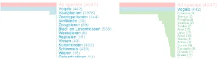
Figure 5: Colour distinguishes between genus (left) and species (right). Barcharts indicate the number of subspecies within each genus/species.
fined amount. Timelines are placed below the maps (Fig.3), but when the mouse is moved over the timeline a histogram that double-encodes the values and time labels are added (Fig.4). The histogram’s use of aligned length provides a better basis for estimating and comparing values than colour lightness and the zooming combined with the Cressman ker-nel enables cycles in decadal, annual and monthly species abundance to be determined.
4.3. Species view
A barchart of the number of subspecies contained within each genus and species accompany the species list, which can be expanded as in Fig.5. Different colours distinguish genus, species and subspecies (red indicates a ‘protected’ status) and they can be ordered by subspecies frequency and in alphabetical order. This zoomable list enables overviews of the hierarchical structure of species taxonomy.
4.4. Selection
As well as providing spatial, temporal and species overviews, each view provides a basis for selection. Fig.6
[image:4.612.312.528.81.221.2] [image:4.612.312.524.288.347.2]obser-A. Slingsby & E. van Loon / Visual Analytics for Exploring Changes in Biodiversity
Figure 6:Screenshot from prototype application. Spatial se-lection and species sese-lections have been applied. A temporal selection (for the past century) is in progress. For this region, the unique number of species observed has been increasing (due to more observations being made over time).
vations exist in the spatial selection) and a temporal selection for the past century being selected (red outline).
Spatial, temporal and species aspects of selections can be saved, named and compared (see next section) as in [SDW11]. These appear on the left of the screen (Fig.6has the default ‘all’ and ‘none’; Fig.7has two more).
4.5. Comparison
The zoomable map, timeline and spatial views along with the selections they facilitate, show spatial, temporal and species distributions of subsets of the data; e.g. the seasonal cycles in species abundance in Fig.4. This is a form of simple com-parison, but does not let us easily look at spatial distributions over time or temporal distributions over space.
Saving selections and then being able to apply these on-demand, allows quick switching between views in Fig. 7
(top), in which 1981 appears to have a higher overall num-ber of species. Such comparison is difficult. To address this, we encode the difference between these directly in Fig.7
(bottom left) by setting the 1980 selection as a baseline. Red indicates that the value was higher in 1981 than 1980. These red areas are stable on map redraws. The timeline is dom-inated by red, indicating that unlike spatially, the species number is consistently higher throughout the year. Using the bionomial proportions statistical test [DeV08] and only colouring parts of the map that are statistically significant (at an 80%p-value) in Fig.7(bottom right), there are geograph-ical areas where this increase is statistgeograph-ically significant.
5. Addressing research questions and ongoing work
[image:5.612.72.287.80.206.2]The graphical representation of spatial and temporal distri-butions of species, the ability to constrain, save and recall se-lections by space, time and species and the ability to have re-sults reported as number of observations, average abundance
Figure 7:Two selections of observations 1980 and 1981 have been saved and can be flipped between (top). Setting 1980 as the baseline, red indicates a higher proportional dif-ference; blue indicates lower (bottom left). On the basis of a binomial statistical test, values that are <80% statistically significant have been removes (bottom right).
or numbers of species present, enables answers to be ob-tained to the research questions listed in section2. A planned workshop with ecologists will help evaluate the success of the design, how initiative the user interface is and whether participants can be confident in the results being reported.
Sampling bias in observation data often requires the use of species distribution models [SP03]. We hope to help es-tablish the degree with which this is true for NDFF – as an example of a large, comprehensive and semantically-rich dataset – using exploratory interactive visualisation. We hope that our findings will help inform the design of sim-ilar databases in future. Sampling bias is perhaps the most significant issue in this work. By identifying systematic sur-veys with species lists in which observation absence implies absence, we hope to explore such sampling bias.
6. Conclusion
References
[Bow00] BOWKERG. C.: Mapping biodiversity. International Journal of Geographical Information Science 14, 8 (2000), 739– 754. URL:http://www.tandfonline.com/doi/abs/ 10.1080/136588100750022769.2
[Bre09] BREWERC.: Colour advice for cartography. http: //www.colorbrewer.org, 2009.3
[COO92] COOPER W.: Cressman analysis. http: //www.asp.ucar.edu/colloquium/1992/notes/ part1/node119.html, 1992.2
[CVC12] CAUDRONA., VIGIERL., CHAMPIGNEULLEA.: De-veloping collaborative research to improve effectiveness in bio-diversity conservation practice.Journal of Applied Ecology 49, 4 (2012), 753–757. URL:http://dx.doi.org/10.1111/ j.1365-2664.2012.02115.x.2
[DeV08] DEVORE J.: Probability and Statistics for Engineer-ing and the Sciences: Enhanced [With Glossary of Symbols Booklet]. Available 2010 Titles Enhanced Web Assign Se-ries. Brooks/Cole, Cengage Learning, 2008. URL:http:// books.google.co.uk/books?id=Wbym40WgsXMC.4
[Fis00] FISHERP. F.: Is GIS hidebound by the legacy of cartogra-phy? Cartographic Journal, The 35, 1 (1998-06-01T00:00:00), 5–9. URL: http://www.ingentaconnect.com/ content/maney/caj/1998/00000035/00000001/ art00002.1
[FLF∗11] FERREIRA N., LINS L., FINK D., KELLING S., WOODC., FREIREJ., SILVAC.: Birdvis: Visualizing and under-standing bird populations. Visualization and Computer Graph-ics, IEEE Transactions on 17, 12 (2011), 2374–2383. doi: 10.1109/TVCG.2011.176.1
[JSRB06] JONESM. B., SCHILDHAUERM. P., REICHMANO., BOWERSS.: The new bioinformatics: Integrating ecological data from the gene to the biosphere.Annual Review of Ecology, Evolution, and Systematics 37, 1 (2006), 519–544. URL:
http://www.annualreviews.org/doi/abs/10. 1146/annurev.ecolsys.37.091305.110031.1
[MBB∗10] MAGURRAN A. E., BAILLIE S. R., BUCKLAND
S. T., DICKJ. M., ELSTOND. A., SCOTTE. M., SMITHR. I., SOMERFIELDP. J., WATTA. D.: Long-term datasets in biodi-versity research and monitoring: assessing change in ecological communities through time.Trends in Ecology & Evolution 25, 10 (2010), 574 – 582.doi:10.1016/j.tree.2010.06.016.
1
[Ope83] OPENSHAW S.: The modifiable areal unit problem, vol. 38. Geo Books Norwich, 1983.3
[SAA∗09] SUTHERLAND W. J., ADAMS W. M., ARON-SON R. B., AVELING R., BLACKBURN T. M., BROAD S., CEBALLOS G., CÔTÉ I. M., COWLING R. M., DA FONSECA G. A. B., DINERSTEIN E., FERRARO P. J., FLEISHMAN E., GASCON C., HUNTER JR. M., HUTTON J., KAREIVA P., KURIA A., MACDONALD D. W., MACKINNON K., MADGWICK F. J., MASCIA M. B., MCNEELY J., MILNER-GULLAND E. J., MOON S., MORLEY C. G., NELSON S., OSBORN D., PAI M., PARSONS E. C. M., PECK L. S., POSSINGHAM H., PRIOR S. V., PULLIN A. S., RANDS M. R. W., RAN-GANATHAN J., REDFORD K. H., RODRIGUEZ J. P., SEYMOUR F., SOBEL J., SODHI N. S., STOTT A., VANCE-BORLAND K., WATKINSON A. R.: One hun-dred questions of importance to the conservation of global bio-logical diversity. Conservation Biology 23, 3 (2009), 557–567. URL: http://dx.doi.org/10.1111/j.1523-1739. 2009.01212.x.1
[SDW11] SLINGSBYA., DYKESJ., WOODJ.: Exploring uncer-tainty in geodemographics with interactive graphics.IEEE Trans-actions on Visualization and Computer Graphics 17, 12 (2011), 2545–2554. URL:http://openaccess.city.ac.uk/ 437/.4
[SP03] STOCKWELLD., PETERSONA.: Comparison of reso-lution of methods used in mapping biodiversity patterns from point-occurrence data. Ecological Indicators 3, 3 (2003), 213 – 221. URL:http://www.sciencedirect.com/ science/article/pii/S1470160X03000451.1,4
[SWI∗09] SULLIVAN B. L., WOOD C. L., ILIFF M. J., BONNEY R. E., FINK D., KELLING S.: ebird: A citizen-based bird observation network in the biological sci-ences. Biological Conservation 142, 10 (2009), 2282 – 2292. URL: http://www.sciencedirect.com/ science/article/pii/S000632070900216X.1
[TC05] THOMAS J. J., COOK K. A.: Illuminating the Path: The Research and Development Agenda for Visual Analyt-ics. National Visualization and Analytics Ctr, 2005. URL:
http://www.amazon.com/exec/obidos/redirect? tag=citeulike07-20&path=ASIN/0769523234.1