Spectral Ranking and Unsupervised Feature Selection for Point, Collective and Contextual Anomaly Detection

(1)

Spectral Ranking and Unsupervised Feature

Selection for Point, Collective and

Contextual Anomaly Detection

by

Haofan Zhang

A thesis

presented to the University of Waterloo in fulfillment of the

thesis requirement for the degree of Master of Mathematics

in

Computer Science

Waterloo, Ontario, Canada, 2014

c

(2)

Author’s Declaration

I hereby declare that I am the sole author of this thesis. This is a true copy of the thesis, including any required final revisions, as accepted by my examiners.

(3)

Abstract

Anomaly detection problems can be classified into three categories: point anomaly detection, collective anomaly detection and contextual anomaly detection [10]. Many al-gorithms have been devised to address anomaly detection of a specific type from various application domains. Nevertheless, the exact type of anomalies to be detected in practice is generally unknown under unsupervised setting, and most of the methods exist in lit-erature usually favor one kind of anomalies over the others. Applying an algorithm with an incorrect assumption is unlikely to produce reasonable results. This thesis thereby in-vestigates the possibility of applying a uniform approach that can automatically discover different kinds of anomalies. Specifically, we are primarily interested in Spectral Ranking for Anomalies (SRA) for its potential in detecting point anomalies and collective anomalies simultaneously. We show that the spectral optimization in SRA can be viewed as a re-laxation of an unsupervised SVM problem under some assumptions. SRA thereby results in a bi-class classification strength measure that can be used to rank the point anoma-lies, along with a normal vs. abnormal classification for identifying collective anomalies. However, in dealing with contextual anomaly problems with different contexts defined by different feature subsets, SRA and other popular methods are still not sufficient on their own. Accordingly, we propose an unsupervised backward elimination feature selection algorithm BAHSIC-AD, utilizing Hilbert-Schmidt Independence Critirion (HSIC) in iden-tifying the data instances present as anomalies in the subset of features that have strong dependence with each other. Finally, we demonstrate the effectiveness of SRA combined with BAHSIC-AD by comparing their performance with other popular anomaly detection methods on a few benchmarks, including both synthetic datasets and real world datasets. Our computational results jusitify that, in practice, SRA combined with BAHSIC-AD can be a generally applicable method for detecting different kinds of anomalies.

(4)

Acknowledgements

First and foremost, I would like to express my heartfelt gratitude to my supervisor, Professor Yuying Li, who have assisted me in every stage of completing this thesis. This thesis would not have been possible without her patience, insightful guidance, and gracious support. Thank you for believing in me.

I would also like to extend my appreciation and gratefulness to my readers, Professor Peter Forsyth and Professor Justin Wan, for taking their precious time to review this thesis. Lastly, my special thanks to every friend that I have met in the Scientific Computing Lab, Kai Ma, Eddie Cheung, Ke Nian, Aditya Tayal, Ken Chan, and Parsiad Azimzadeh for all the wonderful memories.

(5)

4.3.1 BAHSIC-AD . . . 42

4.3.2 A synthetic example . . . 43

5 Computational Results 50 5.1 Benchmark Datasets and Experiment Settings . . . 50

5.1.1 Synthetic Datasets . . . 50

5.1.2 Real World Datasets . . . 51

5.1.3 Experiment Settings and Evaluation Method . . . 54

5.2 Experiment Results . . . 57

(7)

5.2.2 Results on the Real World Data . . . 63

5.3 Feature Ranking Facilitates Interpretation of Ranking Results . . . 68

5.3.1 Feature Importance from Supervised Random Forest . . . 68

5.3.2 Feature Ranking Comparison . . . 69

6 Conclusions and Future Work 71 6.1 Conclusion . . . 71

6.2 Possible Future Work . . . 72

(8)

List of Tables

5.1 Description of synthetic benchmark datasets . . . 52

5.2 Description of real world benchmark datasets . . . 55

5.3 Results on synthetic datasets without feature selection . . . 60

5.4 Results on synthetic datasets with feature selection by BAHSIC-AD . . . 61

5.5 Wesults on real world datasets without feature selection. . . 65

5.6 Results on real world datasets with feature selection by BAHSIC-AD . . . 66

5.7 Top ranked features from supervised random forest and HSIC among 31 features of car insurance dataset . . . 70

(9)

List of Figures

2.1 Examples of different kinds of anomalies . . . 7

2.2 Example of feature-contextual anomalies defined by a feature subset . . . . 9

2.3 Example of confusion matrix . . . 14

2.4 Examples of Receiver Operational Characteristic (ROC) curves. . . 16

3.1 Example of margins and hyperplanes . . . 23

3.2 Example of different label assignments and resultant margins . . . 26

3.3 Graphical illustration of eT_|_z_|_, ₋1 2z T_K_z_{, and} _eT_|_z_{| −}1 2z T_K_z _{. . . .} ₂₉

3.4 Result of SRA on a synthetic example . . . 36

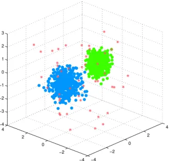
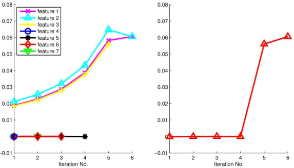
4.1 First two dimensions of toy dataset: two Gaussian clusters with anomalies 45 4.2 Changes of HSICk(˜ Si\I,I) in feature elimination process . . . 46

4.3 Effect of feature selection with BAHSIC-AD on a synthetic example . . . . 48

5.1 Examples of synthetic datasets. . . 53

5.2 Effect of noisy features on different methods . . . 62

5.3 Effect of feature selection with BAHSIC-AD on the performance of different anomaly detection algorithms on real world dataset . . . 67

5.4 Effect of feature selection with BAHSIC-AD on improving interpretabilty of feature ranking resutls . . . 70

(10)

Chapter 1

Introduction

1.1

Motivation

The problem ofanomaly detection is to find the data patterns that deviate from expected normal behavior in a given dataset [10]. The patterns that do not conform with nor-mal pattern are generally referred to as anomalies, and the terms outliers, novelties, and

exceptions are often used interchangeably in literature.

An enormous demand exists for anomaly detection mechanisms from a large variety of application domains, these include but not limited to detecting intrusion activities in network systems, identifying fraud claims in the health or automobile insurance, discov-ering malignant tumor in MSI image, and capturing suspicious human or vehicles from surveillance videos.

The economical value created by successful anomaly detection methods can also be sig-nificant. For instance, insurance fraud has been a severe problem in insurance industry for a considerably long time. While being difficult to estimate the exact loss due to insurance fraud, fraud cases are believed to account for around 10% of total adjustment expenses and incurred losses [27]. The situation is even more severe in certain subcategories. For automobile insurance, this figure goes up to 36% as reported in [14], however, only 3% among them are prosecuted. Since the fraud detection can be modeled as an anomaly

(11)

de-tection problem, substantial loss reduction can be achieved by effective anomaly dede-tection algorithms.

Consider network intrusion detection system [40] [34] as another application of anomaly detection. Almost all contemporary web-based applications, and upper level facilities, require a secure networking infrastructure as their foundation. One important aspect of security is to prevent networking systems from malicious activities. The intrusions include any set of actions that threatens availability or integrity of networking resources. An effective anomaly detection method is evidently crucial for such a system, so that it can keep monitoring the network for possible dangerous misuse and abnormal activities. With anomalies being discovered, alarms can be raised for further actions.

Just as previous examples have shown, reasons for presence of anomalies are usually problem dependent. They can be pure noise introduced in data migration, or misrepre-sented information injected by people with malicious intension. However, despite their differences in actual causes, the main types of anomalies can be broadly categorized into three, i.e. point anomalies, collective anomalies, and contextual anomalies [10]. While many of ad-hoc methods proposed focus on a very specific problem, more studies focus on generic methods that can find a broad type of anomalies (e.g. point anomalies) instead. Although ad-hoc approaches can be more effective for a particular case, their success re-lies on a very good understanding about the nature of the problem. Since attempting to understand the cause of the anomalies, if not impossible, can pose additional complication to the study of the problem, the generic methods which can be applied to detection of different types of anomalies are thereby more desirable in general.

Most of existing anomaly detection methods adopt machine learning techniques, for the reason that machine learning methods are generally very powerful in terms of ex-tracting useful data patterns from the problem with considerable size and complexity [24]. Depending on whether labels are required and how many labels are actually used, these machine learning methods can be further classified into supervised learning algorithms, semi-supervised learning algorithms, and unsupervised learning algorithms. Different from many other applications, where supervised learning normally plays the most important role, a large proportion of anomaly detection problems can only be formulated as unsuper-vised learning problems. This is primarily because of the practical difficulty in acquiring

(12)

labels for many real world applications. Although many unsupervised learning methods have been devised, we usually see strong assumptions made by these methods to detect only a specific type of anomaly. Under these assumptions, the results often favor one type of anomaly over the others. This makes it especially hard for users to choose appropriate unsupervised algorithm when the nature of problem to be addressed is not obvious.

Therefore, we are interested in a more general unsupervised learning method that can handle different kinds of anomalies at the same time. Based on the interpretation presented in [58], Spectral Ranking for Anomalies (SRA) proposed in [37] has the potential to tackle point anomalies and collective anomalies at the same time. Meanwhile, we notice how Hilbert-Schmidt Independence Criteria (HSIC) has the property of capturing arbitrary dependence relationships in a kernel space which can potentially be helpful in feature-contextual anomaly detection. Therefore, based on SRA and HSIC, this thesis proposes an unsupervised learning framework that has the flexibility to adapt to different types of anomaly detection problems with little tuning of parameters.

1.2

Thesis Contribution

This thesis first reviews anomaly detection problem in general by discussing three most common types of anomalies, namely point anomalies, collective anomalies and contextual anomalies. It then reviews prevailing machine learning approaches with a focus on unsu-pervised learning methods. Comments are made on advantages and limitations that are shared in common by these approaches.

The Spectral Ranking for Anomalies (SRA) proposed in [37] is investigated in greater details. In this thesis, we focus on the connection between SRA and unsupervised Support Vector Machine (SVM) as presented in [58]. We demonstrate how spectral optimization based on a Laplacian matrix can be viewed as a relaxation of the unsupervised SVM. Specif-ically, it can be interpreted, under reasonable assumptions, as a constant scaling-translation transformation of an approximate optimal bi-class classification function evaluated at given data instances. Based on this perspective, we justify how SRA has the potential to tackle point anomalies and collective anomalies at the same time by relating different settings of

(13)

SRA to different kinds of anomaly being detected.

We further observe limitations of SRA and other unsupervised methods in handling feature-contextual anomalies on their own. We thereby propose an unsupervised feature se-lection filter scheme, named BAHSIC-AD, based on Hilbert-Schmidt Independence Criteria (HSIC) for the purpose of identifying correct feature contexts of the contextual anomalies. By utilizing the property of HSIC, the proposed method can retain a subset of features that has strong dependence with each other in the implicit feature space. It thereby recon-structs the contexts for approaches like SRA to address the feature-contextual anomalies. With the insight we gain from unsupervised SVM and unsupervised feature selection, we discuss how SRA combined with BAHSIC-AD has the flexibility to handle all three kinds of anomalies with proper assumptions and appropriate problem formulations.

Computational results are presented to compare SRA and other approaches (with or without unsupervised feature selection) for different types of anomaly detection problems. Both synthetic data and real world dataset are utilized to evaluate the methods. We show that SRA can identify both point anomalies and collective anomalies simultaneously and HSIC helps reconstruct the contexts for detecting contextual anomalies. In addition, we take automobile insurance fraud detection as an example to illustrate how feature selection with HSIC also helps in improving the interpretability of the anomaly ranking results.

1.3

Thesis Organization

This thesis is organized as follows:

Chapter2provides the background about different types of anomaly detection problems and reviews the popular machine learning methods to address them.

Chapter 3 investigates the SRA algorithm with the perspective made in [58] which relates SRA with the unsupervised SVM problem. With the connection built with unsu-pervised SVM, it justifies how SRA has the potential in detecting both point anomalies and collective anomalies at the same time.

(14)

SRA and other approaches in handling contextual anomalies with contexts being defined by feature subsets.

Chapter5compares the performance of SRA (with or without BAHSIC-AD) with other anomaly detection methods on both synthetic datasets and real world problems. We also justify how the algorithm improves the effectiveness and interpretability of the anomaly ranking results by studying its performance on an automobile insurance fraud detection dataset.

Chapter 6 concludes the thesis by highlighting the major contributions being made as well as potential directions for future exploration.

(15)

Chapter 2

Background

2.1

Types of Anomalies

Suppose we have a set of m training examples D={x1,x2,· · · ,xm}, wherexi ∈ X ⊆Rd,

the goal of anomaly detection or anomaly ranking is to generate a ranking score f =

{f1, f2,· · · , fm} for each example in D where higher value of fi indicates the instance xi

more likely to be an anomaly.

As discussed in the survey of anomaly detection [10], the most common types of anoma-lies can be classified into three major categories, i.e. point anomaanoma-lies, collective anomaanoma-lies, and contextual anomalies. Point anomaly refers to the individual data instance that clearly deviates from the rest of the dataset. Collective anomalies, on the other hand, refer to the anomalous behavior revealed by a group of data instances. Point anomalies are the most common anomalies discussed and studied in anomaly detection literature whereas the collective anomalies is relatively less encountered but frequently emerged as a rare class classification problem. These two kinds of anomalies are discussed together in Section2.1.1. Lastly, contextual anomaly refers to data instances that are anomalous in a certain context, and not otherwise. Note that, the definition of contextual anomaly requires a clear notion of “context” being defined and the definition of the contexts is crucial for anomalies to be identified. The contexts can be feature subset, data clusters etc. Also, being contextual

(16)

anomaly is not exclusive to other kinds of anomalies, as it is possible to have “contextual point anomalies” and “contextual collective anomalies”. This thesis focuses on contextual anomalies with contexts being defined by feature subset, and we provide our discussions in Section2.1.2.

2.1.1

Point Anomalies and Collective Anomalies

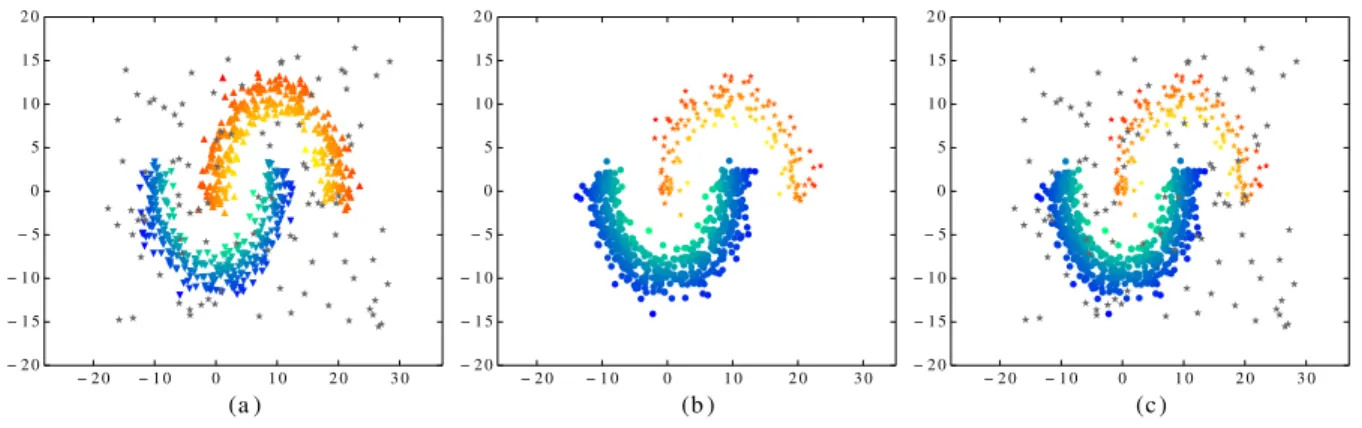
− 2 0 − 1 0 0 1 0 2 0 3 0 (a ) − 2 0 − 1 5 − 1 0 − 5 0 5 1 0 1 5 2 0 − 2 0 − 1 0 0 1 0 2 0 3 0 (b ) − 2 0 − 1 5 − 1 0 − 5 0 5 1 0 1 5 2 0 − 2 0 − 1 0 0 1 0 2 0 3 0 (c ) − 2 0 − 1 5 − 1 0 − 5 0 5 1 0 1 5 2 0

Figure 2.1: Examples of point anomalies (a), collective anomalies (b), and combination of both (c)

Examples of both point anomalies and collective anomalies are presented in Figure2.1. Subplot (a) presents two balanced moon shape clusters, each consists of 500 points. There are additional 100 points (grey stars) uniformly scattered around the two moons which are clearly anomalies with respect to the two major patterns. Therefore, the grey star points can be treated as our examples of the point anomalies. Subplot (b), however, presents two unbalanced moon patterns. The lower moon (blue) consists of 1000 points in total and thereby has much higher mass and density compared with the upper moon (red), which is only of size 300. In this scenario, the lower moon forms the major pattern of the whole dataset. The individual points inside the red moon still lies inside the cluster, and thus cannot be treated as point anomalies. They however collectively form an anomalous pattern that deviates from the major pattern, i.e. the blue moon. This whole group of red points can then be treated as an example of collective anomalies. Subplot (c) shows a

(17)

combination of the two, where we have unbalanced patterns together with random scattered noise. The right subplot in the figure also shows the possibility for the presence of both kinds of anomalies in the same dataset.

2.1.2

Contextual Anomalies

Contextual anomalies is another type of anomalies that is frequently encountered in real world applications. Nevertheless, compared with point anomalies and collective anomalies, it is less studied in general because of the broad concept of “context”. Within same dataset, different data instances can reveal distinctive anomalous behavior with different notion of “context”. Indeed, a data cluster presents in the dataset can be a useful context and a specific feature subset can as well be a meaningful context. Therefore, a proper defined context is required if a reasonable anomaly ranking is expected. Most of successful approaches in literature indeed tended to be ad hoc or tailored for a particular kind of data such as time-series data [45] and spacial data [29] such that the notion of “context” is defined specific to the problem.

In this thesis, we focus on the feature-contextual anomalies with a reasonable assump-tion that different contexts of data correspond to different feature subset. These anomalies are also referred to as conditional anomalies in [51]. The feature-contextual anomalies actually emerge more frequent than people would normally expect. In many real world ap-plications, when people construct the dataset, they normally tend to include features that are potentially relevant at the risk of introducing additional noise. However, this can com-promise the performance of unsupervised anomaly detection algorithms when they simply treat all the features equally.

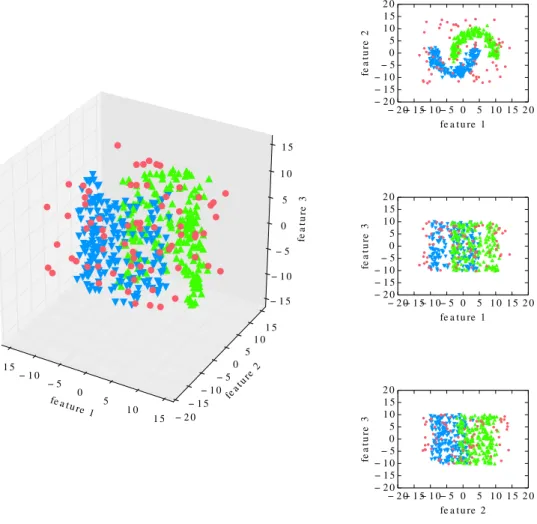
Consider the synthetic data presented in Figure2.2 as an example of feature-contextual anomalies. Suppose we have the following data with three features as shown on the left side of Figure 2.2. The first two features are the noisy two moons which are very similar to the point anomaly dataset presented in Figure 2.1, whereas the third dimen-sion is an additional noisy feature that we have injected into the original dataset. In this case, it is very difficult to identify red points as anomalies when we select subset {f eature1, f eature3} or{f eature2, f eature3}, but they are clear anomalies when we only

(18)

fe a t_{u re} 1 − 1 5 − 1 0 − 5 0 5 1 0 1 5 fea t ure 2 − 2 0 − 1 5 − 1 0 − 5 0 5 1 0 1 5 fe a t u re 3 − 1 5 − 1 0 − 5 0 5 1 0 1 5 − 2 0− 1 5− 1 0− 5 0 5 1 0 1 5 2 0 fe a t u re 1 − 2 0 − 1 5 − 1 0 − 5 0 5 1 0 1 5 2 0 f e a t u r e 2 − 2 0− 1 5− 1 0− 5 0 5 1 0 1 5 2 0 fe a t u re 1 − 2 0 − 1 5 − 1 0 − 5 0 5 1 0 1 5 2 0 f e a t u r e 3 − 2 0− 1 5− 1 0− 5 0 5 1 0 1 5 2 0 fe a t u re 2 − 2 0 − 1 5 − 1 0 − 5 0 5 1 0 1 5 2 0 f e a t u r e 3

Figure 2.2: Example of feature-contextual anomalies defined by a feature subset: noisy two moons with an additional noisy feature

(19)

observe from{f eature1, f eature2}. Although the red points can still be identified with the

full feature set, they are definitely not as clear when we observe from the first two dimen-sions. In this case, it is obvious thatf eature3 adds no value in detecting the anomalies and

the best feature contexts for anomaly detection is the subset features{f eature1, f eature2}.

2.2

Unsupervised Learning for Anomaly Detection

The existing machine learning approaches for anomaly detection in literature can be clas-sified into three broad categories: supervised learning methods, unsupervised learning methods and semi-supervised learning methods. The difference among three categories lies in how many labeled training samples are utilized in the training process. Supervised learning usually requires a full labeled training set. Unsupervised learning, on the other hand, requires no labeled data instance in training. Lastly, semi-supervised operate on the dataset that has only limited number of labeled samples (e.g. only part of normal instances are labeled).

When the labels are actually available, it is generally preferable to apply supervised learning approaches, since the labels can provide additional information about the depen-dence relationship between features and the labels. Nevertheless, a very large number of anomaly detection problems are formulated as unsupervised learning problems instead of supervised learning problems. One important reason for the popularity of unsupervised learning is the implicit assumption made by most of anomaly detection methods [10]. Namely, the normal instances generally account for the majority of the dataset. Therefore, even without the labels, the pattern revealed by majority of the data can be considered as the normal class. Accordingly, many techniques designed for anomaly detection problems fall into the unsupervised learning category.

A more important reason for choosing unsupervised learning is the fact that the clean labeled training data are very scarce for many real world applications. The labels of the data can be difficult or even impossible to obtain due to practical limitations. Consider insurance fraud detection again as an example, people who commit fraud would normally deny their dishonest behavior unless strong evidence is presented. This also implies

(20)

exis-tence of a large portion of unidentified fraud cases in the historical data. Additionally, as time evolves, different types of anomaly emerge. Although supervised learning can best mimic human decisions, they however lack the capability in discovering novel patterns. This can potentially cause oversight of new kinds of fraud behavior. We thereby see the necessity of applying unsupervised learning techniques for these problems.

In the following subsection, we review different unsupervised learning approaches in Section2.2.1 and the common problems they share in Section 2.2.2.

2.2.1

Existing Unsupervised Learning Methods

While there are numerous unsupervised learning methods designed for different tasks, here we review some of the most commonly used approaches along with their applications and assumptions behind them.

Nearest-Neighbor Based Methods

Nearest-Neighbor based methods are among most primitive methods to approach anomaly detection problems. The most basic example is the classical k-Nearest Neighbor (k-NN) global anomaly score. Given a set of training data, the k-NN algorithm finds the k data points that have the smallest distance to each of the data instance, and the score is assigned by either the average distance of the k nearest neighbors [59] [3] [6] or simply the distance to the k-th neighbor [9] [43]. The basic assumption is that, the data point with higher distance to its neighbors is more likely to be an anomaly and the normal instances generally lie closer to its neighbors. While being simple and intuitive, the effectiveness of k-NN methods however depend on the parameterkas well as an appropriate similarity or distance function. The choice of distance function is especially important to make k-NN feasible on the dataset with non-continuous features (e.g. nominal), and we note that several attempts [54] [38] have been made to address the issue .

Density Based Methods

Density based methods are very similar to nearest-neighbor based methods. They also rely on a notion of distance defined over the data and follow similar assumption as the nearest-neighbor based approaches that normal data instances lie in a dense nearest-neighborhood whereas

(21)

anomalous instances usually have a neighborhood with low density. However, instead of taking a global point of view as in nearest-neighbor based methods, density based methods generally only take local density into consideration.

The most commonly used density-based method is Local-Outlier Factor (LOF) as pro-posed in [8]. The local density of a data instance is calculated by first finding the volume of the smallest hypher-sphere that encompass its k-th nearest neighbors. The anomaly score is then derived by taking the average of the local density of its k-nearest neighbor and the local density of the instance itself. The instance in a dense region are assigned a lower score while the instances lie in the low density region will get higher score.

There are many variation of LOF methods that follow similar assumptions. The al-gorithm of Outlier Detection using In-degree Number (ODIN) simply assign the anomaly score as the inverse of the number of instances that have the given instance in their neigh-borhood [25]. An noticeable variation called Local Correlation Integral (LOCI) is proposed in [39]. LOCI claims to detect both point anomalies and a small cluster of anomalies at the same time. One final variation is the local outlier probabilities (LoOP)[30] which improves the interpretability of the ranking score by adopting a more statistically-oriented approach. Clustering Based Methods

Clustering is one major stream of unsupervised learning research and many anomaly detection algorithms are built on top of existing clustering methods. The fundamental assumption behind most clustering based methods is that normal instances should form clusters while anomalies either do not belong to any cluster or lie far away from the closest cluster centroid. A few clustering methods have been proposed with the capability to exclude anomalies (noise) from clustering results, such as Density-based spatial clustering of applications with noise (DBSCAN) [18] and shared nearest neighbors (SNN) clustering [17]. They can also be applied to only identify the anomalies. However, since the methods are originally proposed for the purpose of clustering, they are generally not optimized for the purpose of anomaly detection.

Another clustering-based scheme is based on a two step process. It first applies an existing clustering algorithms (e.g. k-means [32], Self-Organizing Maps [28] or Hierarchical Clustering [35]) to obtain clusters in the data along with the calculated centroids, then the

(22)

anomaly scores are assigned as the distance to the closest cluster centroid. One-Class Classification Based Methods

Anomaly detection problems can also be formulated as one-class classification problems. The basic assumption is that there exists only one class, i.e., the normal class, in the training set. The method then learns a boundary for the normal class, and classifies all the training instances outside the boundary as the anomalies. Examples of this category are the one-class Support Vector Machine (OC-SVM) [47] and one-class Kernel Fisher Discriminants [44], OC-SVM is especially popular for many applications. These methods usually utilize the kernel methods [48] so that they can be generalized to compute non-linear boundaries. Note however, it is not necessary for the training set to be truly one-class (every data instance comes from one class) for algorithms to produce reasonable results. For instance, after transforming the feature using kernel trick, the OC-SVM tries to find the smallest sphere enclosing the data in the space defined by kernel. The dissimilarity to the center of the sphere can then be utilized as the anomaly score.

2.2.2

Limitations of Existing Approaches

There are some common problems shared by the existing unsupervised learning methods in general. Successful unsupervised learning methods require a clear assumption made on the data. However, we see all the unsupervised approaches are based on the assumption that favors one kind of anomalies over the other, and most commonly, they favor towards the detection of point anomalies. This is especially true for most of clustering-based methods and density based methods. Assumptions of these methods generally ignore the possible existence of collective anomalies. Even methods, e.g. LOCI, that do take some special cases of collective anomalies into consideration, they are effective in cases that are specially addressed, such as micro-clusters formed by a very small group of anomalies.

Moreover, we notice that most unsupervised anomaly detection algorithms themselves are generally incomplete in dealing with feature-contextual anomalies. Consider again the example presented in Figure2.2. Under unsupervised learning settings, the potential noisy feature can dramatically compromise the performance of these algorithms if they treated

(23)

all the features equally. In order to handle cases like this, it is necessary to introduce an unsupervised feature selection process whenever it is needed.

2.3

Receiver Operational Characteristic Analysis

Before we dive into the details of SRA, we review the Receiver Operational Characteristic (ROC) Analysis since this will be an important evaluation method for the forthcoming discussion in this thesis.

A ROC graph is a visualization tool for evaluating the performance of various classifiers. Since we are only interested in anomaly detection problems, we illustrate the concept under the settings for anomaly detection. We begin by considering an arbitrary anomaly detector A. Essentially, A is a classifier that maps an input instance x to either positive class, being anomaly, or negative class, being non-anomaly. However, instead of output class membership directly, it is more often the case that A simply generate a continuous output (e.g., an estimate of the probability) indicating the likelihood of this instance being anomaly. Then a threshold is chosen to determine the class membership.

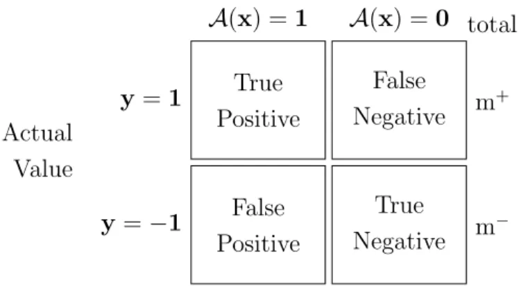
True Positive y=1 A(x) =1 False Negative A(x) = 0 _total m+ False Positive y=−1 True Negative m − Actual Value

Anomaly Detection Outcome

Figure 2.3: Example of confusion matrix

(24)

indeed classified as being anomaly, it is counted as true positive. If it is classified as non-anomaly, it is counted as false negative. Similarly, if x is not an anomaly, but mistakenly classified as an anomaly, it is counted as false positive. If it is correctly classified as non-anomaly, it is a true negative. These quantities are generally summarised in a confusion matrix as shown in the Figure 2.3.

We can then calculate the following metrics based on the classification result, i.e. True Positive Rate (TP Rate),

TP Rate = Anomalies correctly identified Total number of anomalies and False Positive Rate (FP Rate)

FP Rate = Anomalies incorrectly identified Total number of anomalies

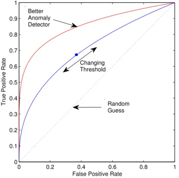
If we vary the threshold, we can obtain different classification results. We thereby obtain a set of pairs ofTP Rate and FP Rate correspond to different threshold values. By plotting the relationship betweenTP Rate and FP Rate, we obtain a ROC graph as shown in Figure2.4.

For anomaly detection problems, if we change the threshold, we can include more data instances as anomalies, but at the risk of falsely including the normal cases. Therefore, we are usually interested in the trade-off between the benefits (higher TP rate) and costs (higher FP rate). This information can be obtained from the ROC graph, even without any prior knowledge about the actual costs due to misclassification. When we have all possible combinations of TP rate and FP rate, real world applications often require an optimal optimal operating point where we set the actual threshold in making the decision. This can be the point on the ROC curve that is closest to the ideal upper left-hand corner or simply the point corresponds to the maximum FP rate that we can possibly tolerate [52]. However, since selecting operating point is really problem dependent, we are more interested in a universal criterion to directly compare different ROCs.

In order to use a single scalar value to compare two or more ROCs generated by different anomaly detectors, it is natural to use the Area Under the ROC Curve (AUC) as the comparison criterion. Since the plot is on a unit square, the value of AUC will always

(25)

lie between 0 and 1.0, and a random guess will result in an 0.5 AUC. Although a ROC has a higher AUC is not necessarily better than one with a lower AUC in a certain region of the ROC plot, the value of AUC is generally a very reliable measure in practice. An important property of AUC is that, it is equivalent to the probability that the anomaly detector ranks a randomly chosen positive instance higher than a randomly chosen negative instance in the given dataset [19]. It is also equivalent to the U statistic in the Mann-Whitney U test as shown in [23].

The AUC will be our main evaluation criterion in Chapter 5, when we compare the performance of different anomaly detection methods.

0 0.2 0.4 0.6 0.8 1 0 0.1 0.2 0.3 0.4 0.5 0.6 0.7 0.8 0.9 1

False Positive Rate

True Positive Rate

Better Anomaly Detector Changing Threshold Random Guess

(26)

Chapter 3

Spectral Ranking for Point and

Collective Anomalies

In this chapter, we analyze and discuss the algorithm of Spectral Ranking for Anomalies (SRA) as proposed in [37]. In Section 3.1, we present the SRA algorithm and discuss the motivation behind it. In Section 3.2, we analyze how spectral optimization based on the Laplacian matrix can be interpreted as a relaxation of an unsupervised SVM. Based on this connection between SRA and unsupervised SVM, we further justify effectiveness of SRA in handling point anomalies and collective anomalies in Section3.3.

3.1

Spectral Ranking for Anomalies

3.1.1

Spectral Clustering

We start our discussion with a brief review on Spectral Clustering [53], which has motivated the SRA algorithm. Spectral clustering has gained its popularity in recent studies of clustering analysis. It has shown to be more effective than traditional clustering methods like k-means and hierarchical clustering. It is especially successful for applications like computer vision and information retrieval [49] [57] [15].

(27)

Suppose we have a set of m training examples D ={x1,x2,· · · ,xm}, where xi ∈ X ⊆

Rd. The goal of spectral clustering is to group data instances into k groups so that data instances in each group are more similar to each other than to those in other groups. Successful spectral clustering relies on a notion of similarity defined over data instances which is provided in the form of a similarity matrix. We denote the given similarity matrix as W ∈ _Rm×m _where _W

ij is the similarity between instance xi and instance xj. Note

however that, the choices for the kernel and similarity measure is problem dependent and not the subject of this thesis. We refer interested readers to [37] for a more detailed discussion on these issues. For the convenience of later discussion, we also let the degree vector d be di =

P

jWij, i= 1,2,· · ·, m, as well asD be the diagonal matrix with d on

the diagonal.

The most important element for spectral clustering is the graph Laplacian matrix. There exist several variations of Laplacian matrices with different properties. The most popular ones include

• Unnormalized Laplacian [49]: L=D−W

• Random Walk Normalized Laplacian [12]: L=I−D−1_W

• Symmetric Normalized Laplacian [36]: L=I−D−12W D− 1 2

As discussed in [53], different variations of spectral clustering algorithms utilize different graph Laplacians. However, the main ideas of these algorithms are similar. Namely, they use graph Laplacians to change the representation of data so that it is easier to determine cluster membership in their new representations. In this thesis, we focus on the symmetric normalized Laplacian for majority of the discussion, and only briefly discuss unormalized Laplacian. Moreover, the symmetric normalized Laplacian is the primary graph Laplacian adopted by our SRA algorithm.

Following the spectral clustering algorithm in [36], an eigendecomposition is performed on the Laplacian matrix L. Assume that the derived eigenvectors are g∗₀,g∗₁,· · · ,g_n−∗ ₁ which are associated to the eigenvalues λ0 ≤ λ1 ≤ · · · ≤ λn−1 respectively. We then use

(28)

the eigenvectorg₀∗,g∗₁,· · · ,g∗_k−₁. After normalizing the rows ofU to 1, we get a new set of representations of the original data instances. More specifically, thei-th row of normalized

U is a new representation of xi in the k dimensional eigenvector space. Finally, we can

apply a traditional clustering algorithm, usually thek-means algorithm, to this new set of representation to figure out the cluster membership.

Note that, each non-principal eigenvector can be regarded as a solution to a relaxation of a normalized graph 2-cut problem. It finds a bi-class partition of the data in the space orthogonal to all previous k −1 eigenvector space. Therefore, spectral clustering can actually be interpreted as a k-step iterative bi-cluster classification method. A more rigorous and detailed discussion is provided in [53], along with other interpretations of spectral clustering.

3.1.2

Spectral Algorithm for Anomaly Detection

Inspired by spectral clustering, Spectral Ranking for Anomalies (SRA) has been proposed in [37] as a novel method to address anomaly detection problems. For practical applications like automobile insurance fraud detection where multiple patterns present as being normal, SRA has shown to be more effective than many traditional anomaly detection methods we have mentioned in Chapter 2, such as one class Support Vector Machine (OC-SVM), Local Outlier Factor (LOF), k-Nearest Neighbor(k-NN) etc. Same as spectral clustering, a similarity matrix is required to capture different characteristics of data and a symmetric normalized Laplacian is needed as the fundamental tool to generate the final ranking. We thereby follow the notation from previous section.

As mentioned in Chapter 2, the objective of anomaly ranking is to generate a ranking

f = {f1, f2,· · · , fm} for each data instance in D where a higher value of fi indicates the

instancexi more likely to be anomaly. Therefore, deciding the cluster membership is not

as important as for clustering analysis and is insufficient for our purpose. However, as discussed in [37], we believe that the first non-principal eigenvector g∗₁ actually has infor-mation beyond merely indicating memberships of data instances, and this inforinfor-mation can be utilized for the purpose of anomaly ranking. Specifically, recall that spectral clustering can be interpreted as an iterative bi-cluster classification process. If we denotez∗ =D12g∗

(29)

we can use |z∗_i| as a measure of how much data instance xi contributes to the bi-class

classification.

To better understand how the values of|z∗| can be helpful in the anomaly ranking, we consider the problem of getting the first non-principal eigenvector ofL. It can be written as the following optimization problem:

min g∈<n g T Lg subject to eTD12g= 0 (3.1) gTg=υ whereυ =Pn i=1di. Since L = I −D−12W D− 1

2 and if we now denote z = D 1

2g and K = D−1W D−1, the

objective function can be transformed in the following manner gTLg = gT(I −D−12W D− 1 2)g = gTg−(D12g)T(D−1W D−1)(D 1 2g) = υ−zTKz

Therefore, if we ignore the constant υ, we have (3.1) in its equivalent form of min

z∈<n −z

T_K_z

subject to eTz= 0 (3.2)

zTD−1z=υ

As discussed in [37], the objective function in (3.2) can be decomposed as sim(C+) + sim(C−)−2×sim(C+,C−)

whereC+={j :zj ≥0},C−={j :zj <0}, sim(C) =

P

i,j∈C|zi||zj|Kij measures similarity

of instance in C (C can be either C+ or C−), and sim(C+,C−) = Pi∈C+,j∈C−|zi||zj|Kij

measures similarity between C+ and C−. The value of the objective function can then be

(30)

z∗, the value of its i-th component |z∗_i| can be used as a strength measure for how much data instancexi contributes to the quality of bi-class classification.

With the bi-class classification strength information provided by |z∗|, we can generate the final rankings for anomaly depends on different scenarios which can possibly be en-countered. The first case is when the data presents multiple major normal patterns. In this case, the data instances correspond to lower value of|z∗_i| are more likely to be anomalies since their memberships to different cluster are more ambiguous than others. Therefore, we can simply usef(xi) = max(|z∗|)− |z∗i| as the ranking function for instancexi.

Another possible situation is when data instances are classified into two classes with normal class being actually clustered into one class and the rest data forms another class. This results in anormal vs. abnormal classification. In this case, the data instances that actually contribute most to theabnormal class are ranked higher. Depends on whether the number of data instances in C+ is higher than that of C−, we can use either f(xi) =−|zi|

orf(xi) = |zi|to rank the anomalies.

To see the meaning of eigenvector more clearly, in next section we present a connection of spectral optimization (3.2) with unsupervised SVM.

3.2

SRA as a Relaxation of Unsupervised SVM

Before we illustrate how SRA can be used to detect point anomalies as well as collective anomalies, we further justify the use of eigenvector for anomaly ranking by illustration spectral optimization problem as an unsupervised SVM.

3.2.1

SVM Revisited

We first revisit the formulation of the standardsupervised maximum margin SVM classifier. While there are other possible equivalent forms of SVMs, we mostly follow the formulation as in [46] and [60].

In a supervised bi-class classification problem, we are given a set of labeled training examples D0 ₌ _{_(x

(31)

hyperplane in_Rd _{is given by}

h(x) =wTx+b = 0

A hyperplane is called a separating hyperplane, if there exists a c such thath satisfies

yi(wTx+b)≥c ∀i= 1,2, . . . , n

Moreover, by scaling w and b we can always get a canonical separating hyperplane, such that

yi(wTx+b)≥1 ∀i= 1,2, . . . , n (3.3)

Suppose two classes in the given dataset are perfectly separable by a hyperplaneh, we then introduce the concept of margin (denoted as γh) of h, as twice the distance between

h to its nearest data instance in D0_{, i.e.}

γ = 2× min

i=1,2,...,nyidi (3.4)

where di is the distance between data instance xi to the hyperplane h. It can be easily

shown that, the distance di is equal to

di =

1

kwk w

T_x i+b)

wherekwk is the Euclidean norm of w. We can then rewrite the margin (3.4) as:

γ = 2× min

i=1,2,...,nyidi =

2

||w||

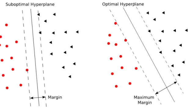
A graphical illustration of margins, maximum margin and their corresponding hyper-planes is provided in Figure3.1.

Intuitively, the best choice, among all hyperplanes that can separate two classes, is the one corresponds to the largest margin. Thereby, a linear hard-margin SVM tries to find the optimal hyperplane which corresponds to the maximal margin between two classes. This solves the following optimization problem:

min w,b 1 2kwk 2_, subject to yi wTxi+b ≥1, i= 1, ..., n,

(32)

Figure 3.1: Example of margins and hyperplanes

However, a perfectly separable dataset is rare in practice. Therefore, we introduce slack variables ξi’s to relax the separability condition in (3.3) when training instances are not

linearly separable, and we have min w,b,ξ 1 2kwk 2₊_C n X i=1 ξi, subject to yi wTxi+b ≥1−ξi, i= 1, ..., n, (3.5) ξi ≥0, i= 1, ..., n ,

where the regularization weight C ≥ 0 is a penalty, associated with margin violations, which determines the trade-off between model accuracy and complexity. The optimal decision function then has the following form

h(x) = n X j=1 yjαjxTxj +b ! .

The SVM discussed so far is just a linear classifier, which has very limited power in many situations. The “kernel trick” is utilized to cope with more complicated cases. Suppose

(33)

we have φ : X 7→ F which is a non-linear feature mapping from input space X to a (potentially infinite dimensional) feature spaceF derived from feature inputs. To find the optimal hyperplane in the feature space, we formulate a kernel soft-margin SVM, which solves the following optimization problem:

min w,b,ξ 1 2kwk 2₊_C n X i=1 ξi, subject to yi wTφ(xi) +b ≥1−ξi, i= 1, ..., n, (3.6) ξi ≥0, i= 1, ..., n ,

with the optimal decision function

h(x) = n X j=1 yjα∗jφ(x) T_φ_(x j) +b∗ ! where (a∗, b∗) is a solution to (3.6).

Recall that the SVM problem (3.6) is a convex quadratic programming (QP) problem which satisfies the strong duality. This means that an optimal solution to (3.6) can be computed from its dual form

max α αα − 1 2 n X i,j=1 yiyjαiαjφ(xi)Tφ(xj) + n X i=1 αi subject to 0≤αi ≤C, i= 1,· · ·, n (3.7) n X i=1 αiyi = 0,

By observing the dual problem (3.7), we notice that we can use the inner product

φ(xi)Tφ(xj) in the objective function to solve the problem without explicityly knowing

what φ is. In general, we can consider a Kernel Function K : _Rd _×

Rd 7→ R such that

K(xi,xj) = hφ(xi), φ(xj)i = φ(xi)Tφ(xj),∀i, j = 1,2,· · · , n. Accordingly, the n-by-n

matrix K with Kij = K(xi,xj) is called a Kernel Matrix. Therefore, by simply utilizing

different kernel, such as polynomial kernel

K(xi,xj) = xTi xj + 1

(34)

or Gaussian radial basis function (RBF) kernel

K(xi,xj) = e

kx_i−x_jk2

σ2

we can find the optimal hyperplane in the implicit feature space induced by the corre-sponding kernel and thereby give SVM a lot more generality. Note that, the necessary and sufficient condition forK to be a valid kernel (also called a Mercer kernel) is that the corresponding kernel matrixK is symmetric positive semidefinite for any {x1,x2,· · · ,xn}

with any n [26]. We assume K is a valid kernel for all upcoming discussions.

Finally, we denote Y =diag(y), and the dual problem of a SVM (3.7) with an

(possi-bly) non-linear kernel can be rewritten into the following matrix form:

max α αα − 1 2ααα T_{Y KY α}_α_α₊_eT_α_α_α subject to 0≤αi ≤C, i= 1,· · ·, n (3.8) yTααα= 0

3.2.2

Unsupervised SVM

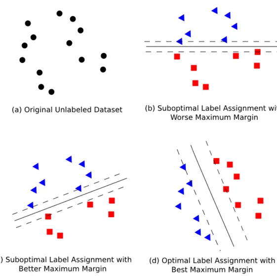
For unsupervised SVM learning, we are given the data instances without labels. The goal then becomes finding the optimal label assignment for dataset such that the resultant hyperplane from supervised SVM has the maximal margin. Figure 3.2 gives an intuitive graphical illustration about how different label assignments can affect the maximum margin found by SVM.

Specifically, an unsupervised SVM is to find the labels yso that the objective value in (3.6) is minimum. Formally, this solves the following nested minimization problem:

min yi∈{±1} ( min w,ξ,b,yi(wTφ(xi)+b)≥1−ξi,ξi≥0 1 2kwk 2 2+C n X i=1 ξi ) (3.9)

(35)

(36)

Since we know the inner convex optimization problem satisfies strong duality, we can replace it by its dual problem and get the following equivalent minmax problem

min yi∈{±1} max 0≤_αi≤C yT_α_α_α₌₀ −1 2ααα T Y KY ααα+eTααα (3.10)

Recall our discussion in previous section about supervised SVM, we now introduce another transformation of (3.8) as this will useful for the forthcoming discussions. If we introduce vector z∈_Rn _{such that}

zi =αi·yi, i= 1,· · · , n

we have

αααTY KY ααα=zTKz, and yTααα =eTz Moreover, for any αi 6= 0, we have

yi = sign(zi), i= 1,· · · , n (3.11)

which also implies

eTα=eT|z|

Therefore, the optimization problem in (3.8) is also equivalent to max z e T_|_z_{| −} 1 2z T_K_z subject to eTz= 0, (3.12) |z| ≤C

We however notice the objective function in (3.12) is no longer concave, and it has many local maximizers. Since (3.12) is equivalent to the dual of the inner optimization problem in (3.10). Therefore, (3.10) can also be written as

min yi=sign(zi) max eTz=0 |z|≤C eT|z| − 1 2z T_K_z _(3.13)

(37)

Now consider the following problem with a rectangular constraint min z − 1 2z T_K_z subject to eTz= 0, (3.14) |z| ≤C

AssumeK is positive definite in the space {z:eTz= 0}, and all local minimizers of (3.14) are at the boundary of |z| ≤ C. Also, assume all local maximizers of (3.14) have the same value for the termeT|z|, then we can “simplify” the unsupervised SVM (3.13) to the minimization problem (3.14).

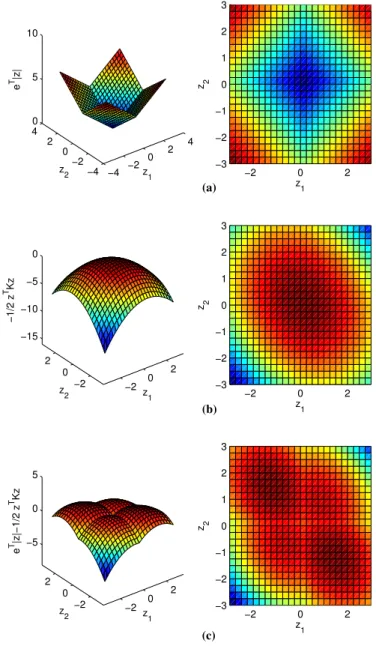
To better understand why relaxation (3.14) is reasonable, we consider following example with graphical illustrations. An examples of possible shapes of functions eT_|_z_|_, ₋1

2z

T_K_z,

and eT_|_z_{| −} 1 2z

T_K_z _{in two dimensional case are depicted in Figure} _3.3 _{(a), (b), and (c)}

separately. For all plots, thex-axis andy-axis are the values ofz1 andz2 separately. Recall

the problem of unsupervised SVM, we are only interested in the label assignment ofz1 and z2 such that we find the minimum of local maximums. In this two-dimensional case, we

observe there are four local maximum as shown in Figure 3.3 (c). However, these actually correspond to only two cases, i.e. signs of z1, z2 are the same, or they are different. The

case that sign(z1) = sign(z2) corresponds to the upper right and lower left regions in the

heatmap whereas sign(z1) 6= sign(z2) corresponds to upper left and lower right regions.

We note that the minimum of these local maximums is the case where sign(z1) = sign(z2),

namely, optimal choice of z should lie in the upper right and lower left regions to the origin. By observing the Figure3.3(b), we notice these are also the directions that function

−1

2z

T_K_z _{drops fastest. On the other hand, Figure} _3.3 _{(a) shows that} _eT_|_z_| _{elevates the}

values in same fashion on all four directions. These observations suggest that the best label assignments y for the minmax objective function (3.13) are simply the signs of z that decreases fastest in the objective function of (3.14). Therefore, we can simply ignore the label assignment and change our objective to finding the minimum of−1

2z

T_K_z _under

the same constraints. In other words, we can change our objective function from (3.13) to (3.14) and simplify our problem in the aforementioned manner.

Note however, (3.14) remains an NP-hard problem since it is trying to find minimum of a concave objective function with rectangular constraint.

(38)

−4 −2 0 2 4 −4 −2 0 2 4 0 5 10 z 1 z₂ e T|z| −2 0 2 −3 −2 −1 0 1 2 3 z 1 z2 −2 0 2 −2 0 2 −15 −10 −5 0 z₁ z₂ −1/2 z TKz −2 0 2 −3 −2 −1 0 1 2 3 z 1 z2 −2 0 2 −2 0 2 −5 0 5 z₁ z₂ e T|z|−1/2 z TKz −2 0 2 −3 −2 −1 0 1 2 3 z 1 z2 (c) (b) (a)

Figure 3.3: Graphical illustration of eT_|_z_|_,₋1 2z

T_K_{z, and} _eT_|_z_{| −} 1 2z

(39)

3.2.3

Connection between Spectral Optimization and

Unsuper-vised SVM

Recall the optimization problem (3.1) for finding first non principal eigenvector is equivalent to min z∈<n −z T_K_z subject to eTz= 0 zTD−1z=υ

as presented in (3.2). Assuming K is positive definite, then we can replace the ellipsoidal equality constraint by an inequality constraint

min z∈<n −z T Kz subject to eTz= 0 (3.15) zTD−1z≤υ

because the ellipsoidal constraint in (3.15) should be active at a solution. Assume that we have K = D−1_{W D}−1 _and _C ₌ _υ _·_d1₂_{, we notice the problem (}_3.15_{) can actually be}

considered as an approximation to the optimization problem (3.14) by approximating the rectangular constraint in (3.14) by the ellipsoidal constraint in (3.15).

This suggests that the normalized spectral optimization problem (3.1) can be re-garded as an approximation to the unsupervised SVM problem (3.10) with the kernel

K =D−1_{W D}−1 _and _C ₌_υ_·_d1₂_.

Since the optimal separating hypothesis from the unsupervised SVM has the form

h(x) = n X j=1 y_j∗α∗_j ·K(x,xj) +b∗ !

and a non-principal eigenvector of the normalized spectral clustering z∗ yields an approx-imation|z∗| ≈ α∗ and _sign(z∗)≈ y∗, which are the coefficients of the bi-class separating optimal decision function,|z∗_j|provides a measurement of the strength of support from the

(40)

jth data point on the two class separation decision. We note however that, because of the use of the ellipsoidal constraint rather than rectangular constraints and other approxima-tions, z∗ is different from the exact SVM decision function coefficients. Specifically, the components of eigenvector are mostly nonzero which suggests every data instance provides certain level of support in this two clusters separation.

In addition, assume that g∗₁ is the first non-principal eigenvector of a variation of un-normalized Laplacian L = I −W, with the eigenvalue λ1. Then we have K = W and

z∗₁ =g₁∗. Under this assumption, it can be easily verified that

Kz∗₁ = (1 +λ1)z∗1. Consequently (1 +λ1)z∗1 =Kz ∗ 1 ≈       f(x1) f(x2) .. . f(xn)       −b∗

Therefore z∗₁ can as well be interpreted as a constant scaling-translation mapping of the approximate optimal bi-class separation function f(x) evaluated at data instances. In this case, it is reasonable to use spectral optimization solution z∗ as the ranking for the bi-cluster separation.

One remaining issue about SRA is to choose right ranking function based on the results of spectral optimization. As discussed in Section 3.1.2, two different rankings can be generated by SRA, i.e. f(xi) = max(|z∗|)− |z∗i| for the case that multiple normal patterns

present, andf(xi) =|zi| for a normal vs. abnormal classification. To choose appropriate

ranking, SRA simply introduces an input parameter χ as a user-defined upper bound of the ratio of anomaly. If the bi-class classification results in two very unbalanced clusters, it is very likely that we are facing the second scenario. We then report the ranking respect to a single major pattern and output an mFLAG = 0. On the other hand, if each class actually accounts for sufficient mass, it is more likely to be formed by other major normal patterns. Thereby, the ranking with respected to multiple major patterns is reported as in the first case with mFLAG set to 1.

(41)

Algorithm 1: Spectral Ranking for Anomalies (SRA) Input: W: Anm-by-m similarity matrix W.

χ: Upper bound of the ratio of anomaly

Output: f∗ ∈ <m_{: A ranking vector with a larger value representing more abnormal}

mFLAG : A flag indicating ranking with respect to multiple major patterns or a single major pattern

begin

Form Laplacian L=I−D−1/2_{W D}−1/2 _;

Compute z∗ =D12g∗

1 where g

∗

1 is the 1st non-principal eigenvector for L ;

Let C+ ={i:z∗i ≥0} and C− ={i:z ∗ i <0}; if min{|C+_m|,|C−| m } ≥χ then mFLAG = 1,f∗ = max(|z∗|)− |z∗| ; else if |C+|>|C−| then mFLAG = 0,f∗ =−z∗ ; else mFLAG = 0,f∗ =z∗ ; end end

(42)

3.3

Detecting Point Anomalies and Collective

Anoma-lies with SRA

Although not specifically addressed, it has been demonstrated in [37] that SRA is capable of detecting point anomalies and collective anomalies at the same time. In this section, we further justify this fact and investigate the performance of SRA on different cases by taking the perspective based on its connection with the unsupervised SVM.

In order to examine the performance of SRA, we apply SRA to the two moon synthetic datasets presented in Figure 2.1 from the previous chapter, as they cover several typical scenarios of anomaly detection problems. In addition, the two moons are intuitive but non-trivial examples of bi-class classification problems. Therefore, by applying SRA on these datasets, we can see the performance of SRA as both an anomaly detection method as well as an unsupervised SVM classifier.

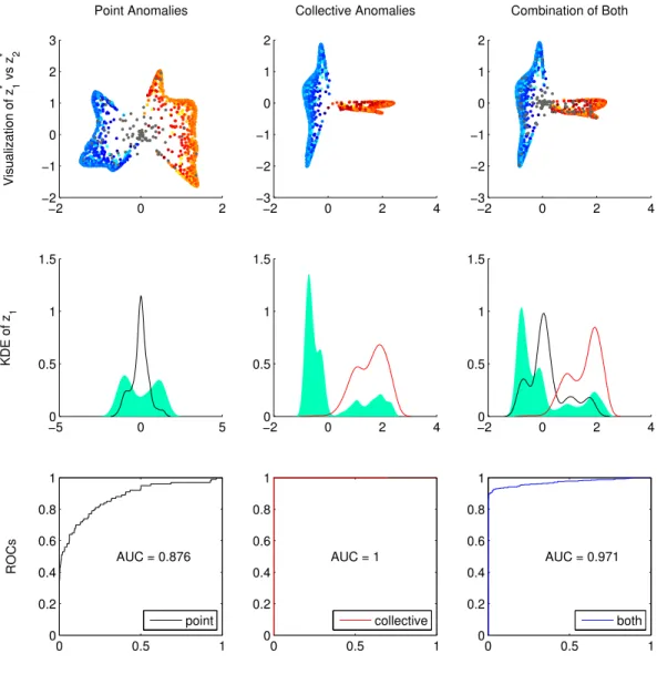
The results we obtained by applying SRA on these synthetic datasets are provided in Figure3.4. The first row of the plots presents the information contained in the first and second non-principal eigenvectors of the normalized Laplacian matrices L’s. It shows the relationship between z∗₁ =D12g∗ 1 and z ∗ 2 =D 1 2g∗ 2 where g ∗ 1 and g ∗

2 are the first and second

non-principal eigenvectors, and the corresponding points are depicted with the same color as in Figure 2.1. It can be seen, in all three cases, how the points from two moons are separated by x= 0 on the x-axis which is in accordance with a bi-cluster separation in the unsupervised SVM. The points are classified into a positive class C+ and a negative class

C− which encapsulates the points of red moon and blue moon separately.

In order to illustrate different behavior of different kinds of anomalies in the ranking results, we consider only the 1st non-principal eigenvector and apply kernel density esti-mation (KDE) to the points corresponding to whole dataset (green shaded area) as well as only subsets of points corresponding to specific types of anomalies, i.e. the point anomalies (black curve) and collective anomalies (red curve). The results are given in second row of Figure 3.4. For all these cases, the score vector z∗₁ derived from the 1st non-principal eigenvector presents a roughly multi-modal pattern with at least one noticeable peak on each side of the origin. We also notice that, the point anomalies are generally close to the

(43)

origin as the highest peak of its KDE is right around 0. This also conforms the intuition gained previously, as |z∗| provides a bi-class clustering strength measure and a smaller value suggests more ambiguity in terms of identification of the instance, therefore more likely to be the anomalies we are detecting. For the unbalanced case without additional noise, we notice how the 1st eigenvector perfectly separates the points and the curve cor-responds to the positive class C+ perfectly aligns with the distribution of the rare class,

i.e. the collective anomalies we defined. For the last case where both anomalies exist in the data, the general principal also holds, as the peaks of the green shaded area have their clear meaning: The highest peak of C− corresponds to the majority pattern whereas the

peak around 0 is related to the point anomalies, and the positive class still corresponds to the collective anomalies.

The above observations also relate different values of resultant mFLAG to different types of anomalies discovered. An output value of mFLAG = 0 would normally indicate the possible existence of the collective anomalies identified by SRA. Moreover, if both types of anomalies are present in the data at the same time, we notice the collective anomalies are ranked higher due to their stronger contribution to the “abnormal” class. This also suggests that mFLAG can be preset as an input to target a specific kind of anomaly. For instance, if we only want the ranking for point anomalies, we can simply set mFLAG = 0 and thereby ignore the ranking for collective anomalies. These observations justify that SRA has the capability of detecting collective anomalies and point anomalies simultaneously. It possesses the generality to detect different kinds of anomalies without the prior knowledge about the type of anomalies to be detected, and also retains the flexibility to let users determine what specific kind of anomalies they are interested in. This is especially valuable under unsupervised setting, as most other methods relies on the assumptions that only favor a specific kind of anomalies.

To justify the actual ranking quality obtained by SRA, we utilize the Receiver Operating Characteristic (ROC) curve as discussed in Section2.3. The resultant ROC for each case is depicted on the last row of Figure 3.4. It can be seen that the collective anomalies can be perfectly tackled, as we can see a perfect normal vs. abnormal classification in the first non-principal eigenvector. The performance in terms of point anomalies is also remarkable considering the fact that the anomalies are not perfectly separable from normal

(44)

data instances due to the way they are generated. Finally, if we consider the case of targeting both at the same time, we can still obtain a nearly perfect overall ROC.

(45)

−2 0 2 −2 −1 0 1 2 3 Point Anomalies Visualization of z 1 * vs z 2 * −50 0 5 0.5 1 1.5 KDE of z 1 * 0 0.5 1 0 0.2 0.4 0.6 0.8 1 ROCs AUC = 0.876 point −2 0 2 4 −3 −2 −1 0 1 2 Collective Anomalies −2 0 2 4 0 0.5 1 1.5 0 0.5 1 0 0.2 0.4 0.6 0.8 1 AUC = 1 collective −2 0 2 4 −3 −2 −1 0 1 2 Combination of Both −20 0 2 4 0.5 1 1.5 0 0.5 1 0 0.2 0.4 0.6 0.8 1 AUC = 0.971 both

Figure 3.4: Result of SRA on the synthetic data shown in Figure 2.1. First row shows z∗₁ (x-axis) and z∗₂ (y-axis) based on first and second non-principal eigenvectors. Sec-ond row shows kernel density estimation of z∗₁ over all dataset(green shaded area), point anomalies(black) and collective anomalies(red). Third row shows the ROC curves and corresponding AUCs.

(46)

Chapter 4

Unsupervised Feature Selection with

HSIC to Detect Contextual

Anomalies

In this chapter, we propose an unsupervised feature selection scheme based on the Hilbert-Schmidt Independence Criterion (HSIC) for the purpose of detecting feature-contextual anomalies. This chapter is divided into the following sections. In Section 4.1, we discuss how the feature selection for anomaly detection is different from other feature selection problems and the key assumption behind our proposed algorithm. In Section 4.2, we review the definition of HSIC and its application for the supervised feature selection. In Section 4.3, we present an unsupervised feature selection scheme based on HSIC that is useful for detecting contextual anomalies.

4.1

Feature Selection for Anomaly Detection

Extensive research has been conducted on the subject of supervised feature selection[22] [41] [31], and many attempts have been made for the unsupervised clustering as well [16]. In general, unsupervised feature selection can be very difficult because of the absence of

(47)

label information. With different selection criterion, the resultant feature subset can be significantly different and thereby greatly distort the performance of underlying algorithms. Moreover, most of existing unsupervised feature selection methods are not suitable for anomaly detection problems, as they mostly focus on searching the subset of features that results in best clustering quality, which is very different from the objective of anomaly detection.

Comparing with clustering analysis, feature selection can be even more challenging for anomaly detection problems due to the possible intervention from both unnecessary fea-tures and anomaly data instances. Additionally, intrinsic questions in real world problems inevitably inject uncertainty in the process of constructing features for training. Consider again the insurance fraud detection example discussed in Chapter2, it is generally hard to target the exact relevant subset of features since adjusters or fraud experts tend to include more potential useful features at the risk of introducing noise. Consequently, we need a clear objective and reasonable assumptions to make feature selection possible for anomaly detections.

Recall different kinds of anomaly detection problems we have discussed so far, despite their differences, the abnormality are all defined over certainnormal property that present in other data instances. This provides certain insight for us to approach the feature selec-tion problem. Especially, when we are aware of the potential existence of noisy or unrelated features in the provided training dataset, we are most interested in the subset of features that can best reveal the structure of the data. In other words, we are interested in the subset of features the are actually useful for detecting anomalies. A reasonable assumption is that, a useful context is constructed by interactions among a subset of features and the interaction can be captured by a certain kind of dependence relationship among these fea-tures. For the noisy features, they should have no dependence with others, and the features that are not very helpful in constructing contexts should also have very limited dependence with other features. In summary, for the purpose of detecting feature-contextual anomalies, our objective is to reconstruct correct contexts for anomalies by eliminating the features that have little dependence relationship with others.

(48)

4.2

HSIC and supervised feature selection

To achieve the goal of effective feature selection for anomaly detection, we utilize Hilbert-Schmidt independence criterion (HSIC) as a fundamental tool in detecting dependence relationship among features. HSIC was proposed in [21] as a measure of statistical depen-dence and was first used for supervised feature selection in [50]. To prepare subsequent discussion, this section reviews the definition of HSIC and its useful properties that are helpful in feature selection. The presentation mainly follows [21] and [50].

Before we discuss detection of arbitrary dependence among data using HSIC, we first consider a simple case of detectinglinear dependence among data. Following similar nota-tions as previous chapters, assume that we have two feature domainsX ⊂_Rd _and_{Y ⊂}

Rl, and we have random variables (x, y) that are jointly drawn from X,Y. Then we denote the cross-covariance matrix of x, y asCxy, and we have

Cxy =Exy

xyT−_Ex[x]Ey[y]

We know that Cxy contains all the second order dependence between x and y, and the

Frobenius norm ofCxy is defined as the trace of CxyCxyT , namely

kCxyk2Frob= tr CxyCxyT

which summarizes the degree of linear correlation between x and y. The value ||Cxy||2Frob

is zero if and only if there is no linear dependence between x and y, and this can thereby be utilized in detecting linear dependence between them. However, capturing only linear dependence is rather limited, especially when we are uncertain about the actual type of data we are dealing with, and the dependence relationship might not be captured by cross-covariance at all. Instead, we are interested in the flexibility of detecting arbitrary dependence, possibly nonlinear dependence, relationship between x and y. We thereby generalize the notion of cross-covariance to detect nonlinear relationship and to cope with different kinds of data.

In order to handle nonlinear cases, we introduce two feature mappings φ : X → F

(49)

Hilbert spaces F and G. The inner product between features can then be rewritten via their characteristic kernel functions

k(x, x0) = hφ(x), φ(x0)i and l(y, y0) =hψ(y), ψ(y0)i

Issues concerning of kernels are usually similar to the kernels selections for SVM as dis-cussed in previous Chapter. Examples include polynomial kernel and Gaussian RBF kernel that map data to higher dimensional spaces. Following [20] and [5], we then generalize the idea of cross-covariance matrix and define a cross-covariance operatorCxy :G → F between

the feature maps such that

Cxy =Exy h φ(x)−_Ex[φ(x)] ⊗ φ(y)−_Ey[ψ(y)] i

and ⊗denotes the tensor product. Denote the distribution for sampling x and y as P rxy,

HSIC is then defined as:

HSIC(F,G, P rxy) =kCxyk2HS

wherek·kHS is the Hilbert-Schmidt norm. The Hilbert-Schmidt norm is used here to extend

the notion of Frobenius norm to operators, and similarly it has the form of tr CxyCxyT

. If we rewrite this measure in terms of kernel functionsk and l, we have:

HSIC(F,G, P rxy) =

Exx0_yy0[k(x, x0)l(y, y0)] +_E_xx0[k(x, x0)]_E_yy0[l(y, y0)]−2_E_xy_E_x0[k(x, x0)]_E_y0[l(y, y0)] (4.1)

One advantage of HSIC is that it is very easy to estimate. Two most popul