Non thermal galactic background radiation

NON-THERMAL GALACTIC

BACKGROUND RADIATION

by

H.V. Cane, B.Sc. (Hons.)

submitted in fulfilment of the requirements for the degree of

Doctor of Philosophy

UNIVERSITY OF TASMANIA HOBART

This thesis contains no material which has been submitted or accepted for the award of any other degree or diploma in any university.

To the best of my knowledge and belief, the thesis contains no copy or paraphrase of material previously published or written by another person, except where due acknowledgement is made in the text.

ABSTRACT

This thesis presents the results and analysis of data obtained using the Llanherne low-frequency array. Surveys of the Galaxy at five frequencies in the range 2 to 20 MHz have been made and the data have been assembled into maps covering the area

3200 < k < 30° and -25° < b < 22°. The data from these maps are

combined with data from seven earlier continuum surveys to produce galactic radio spectra in various directions.

A summary is made of most of the measurements, at frequencies less than approximately 400 MHz, 'of the galactic background radiation and their interpretation. Two new composite maps, at 10 and 30 MHz, are presented. These, combined with the 85 MHz all-sky map, are

used to illustrate the variation of the galactic non-thermal radiation across the sky, and with frequency.

The galactic spectra are interpreted in terms of a model of the Galaxy in which synchrotron emission, and absorption in HII regions predominate in spiral arms. However, it is proposed that the synchrotron emission arms and the arms defined by HII regions are not coincident. In addition to the HII absorbing gas the model incorporates a much broader uniform absorbing HI gas which is

responsible for high latitude absorption, pulsar signal dispersion and Faraday rotation.

For the HI gas it is found that

f

ne2 Te-1 . 35 dl = 1.1 x 10

-7 cm-6 K-1.35 pc

For the HII gas the above quantity varies for different arms. An

average value is

f

CONTENTS

CHAPTER 1 - INTRODUCTION

Preface ₁

Acknowledgements

CHAPTER 2 - EMISSION AND ABSORPTION MECHANISMS

Introduction 5

Synchrotron Emission 6

Thermal Absorption 9

Low Energy Electron Cut-off 14

The Razin Effect 17

References 20

CHAPTER 3 - LIMITATIONS TO LOW FREQUENCY RADIO ASTRONOMY

Introduction 21

Ionospheric Limitations 24

Transmitting Station Interference 28

Limitations on Absolute Calibrations 28

References 30

CHAPTER 4 - THE INTERSTELLAR MEDIUM

Introduction 31

HII Regions 31

The HI Distribution 35

Diffuse Ionized Hydrogen 36

The Galactic Magnetic Field 46

CHAPTER 5

Introduction 57

PART I - GALACTIC BACKGROUND RADIATION

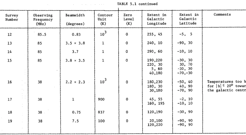
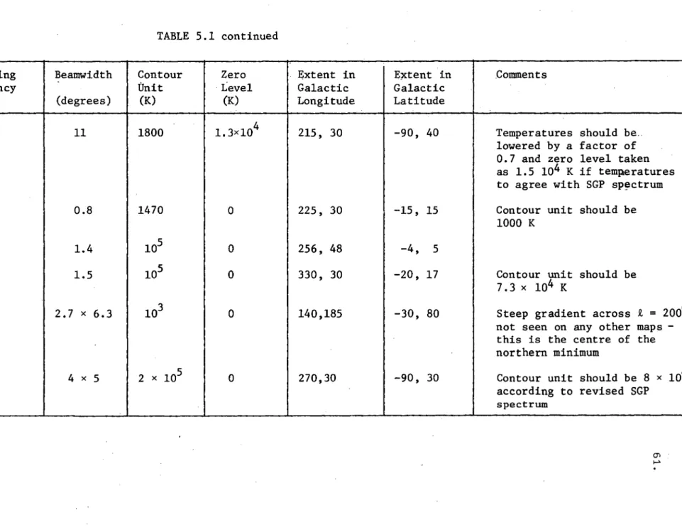
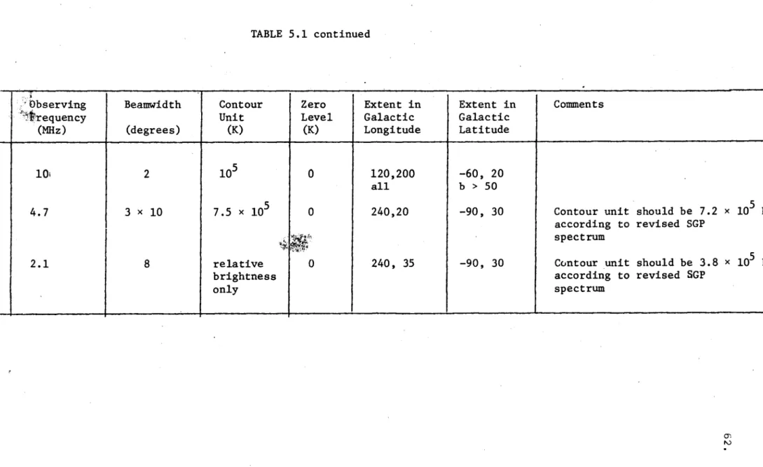
Sky Surveys 58

The 10 MHz Composite Map 64

The 30 MHz Composite Map 67

The Distribution of the Non-Thermal Background Radiation 70

PART II - GALACTIC SPECTRA

The Spectra of the Galactic Polar Regions 85

Discussion 99

Galactic Spectra in Other Directions 102

PART III - SPECTRAL INDEX VARIATIONS

Introduction 107

The Measurements 108

Variations of the Total Background Temperature

Spectral Index 110

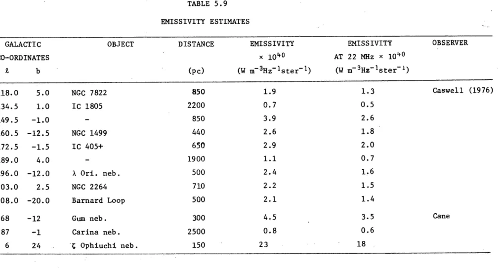
PART IV - NON-THERMAL EMISSIVITY

Introduction 118

The Measurements 118

Cosmic Ray Electron Spectrum 129

References 133

CHAPTER 6 - THE RESULTS

Introduction 137

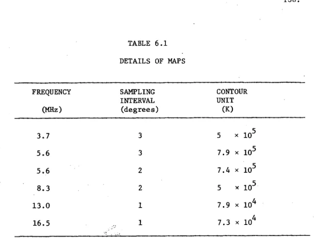
Data Preparation 137

Scans 139

Maps 139

CHAPTER 6 - continued

Galactic Background Spectra 169

Discussion 180

References 18.2

CHAPTER 7 - THE LOW FREQUENCY ANALYSIS

Introduction 183

Previous Investigations 183

The Model 186

Results 194

Discussion - Emission Properties 200

- Absorption Properties 203

Summary 205

References 206

CHAPTER 8 - FUTURE OBSERVATIONS 208

APPENDIX I - THE GUM NEBULA

Discussion 212

References 216

APPENDIX II - INSTRUMENTATION

Introduction 217

The Array 217

The Phasing 220

Receiving Equipment 223

Observing Procedure 227

1.

CHAPTER I

INTRODUCTION

Preface

This thesis is a description of the features of the

galactic background radiation at frequencies below about 400 MHz.

The first four chapters present review material. In Chapter 2

we discuss the emission and absorption processes relevant to the

work. Chapter 3 covers the problems peculiar to low frequency

astronomy. In Chapter 4 we review the observations of the interstellar

medium. In this the major objective is to determine the properties

and distribution of free electrons in the Galaxy.

Chapter 5, which contains some original work, is relatively

long and has been divided into four parts. In Part I we present a

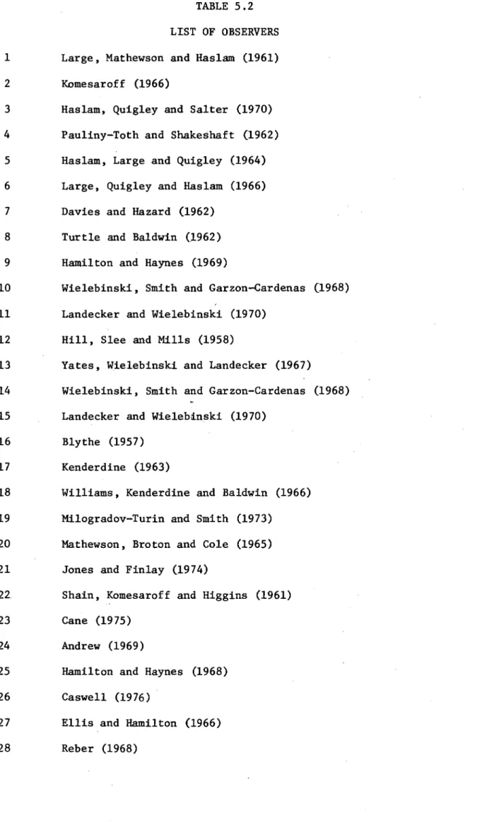
catalogue of sky surveys at frequencies less than about 400 MHz

and two new composite maps at 10 and 30 MHz. These data are used to

discuss the properties of the background radiation. In Part II all

the polar spectral points of both polar regions are presented and

new polar spectra defined. In addition, spectra for the

anti-centre and northern minimum directions are defined. In Part III

spectral index variations are discussed. This includes a review of

previous investigations and some new work using three composite

maps. Part IV is a discussion of the results from emissivity

estimates. Measurements are tabled, and plotted in several forms.

Chapters 6 and 7 present the major original contribution

of this thesis. Chapter 6 comprises the experimental part and

presents the data obtained using the Llanherne array in the form

of declination scans and maps. Spectra are then compiled using

seven earlier continuum surveys. These spectra exhibit unusual

these spectra which is also compatible with the conclusions of

Chapter 5.

In Chapter 8 the uncertain areas in galactic background

radiation studies are discussed and measurements suggested to

clarify some of the uncertainties.

The thesis concludes with two appendices. The first is a

brief summary of the recent work on the Gum Nebula and includes

some comments on an early publication by the author.

The second appendix deals with the instrumentation used

to obtain the sky surveys. This is included as an appendix

because the author was not connected with the majority of the

design of the array or receiving equipment. The description of

the phasing is included in some detail as the author was responsible

for part of the design and because it has not been documented

elsewhere.

3.

Acknowledgements

This project was initiated by Professor G.R.A. Ellis

and his assistance as supervisor is acknowledged.

During the first four years financial support was provided

by a Commonwealth Postgraduate Scholarship. Afterwards support

was provided by the A.F.U.W. and Zonta International.

Technical assistance was provided by a number of people

but in particular by Mr. G. Gowland and Mr. P. Button.

The project would not have been as successful without the

introduction and utilization of the PDP-8 computer. The interfacing

and installation was performed by Mr. G. Gowland and the software

written by Mr. P.S.Whitham. Mr. P.S. Whitham also wrote the

software for the sky observing program and willingly provided

assistance with its implementation.

The contour plotting program used to draw the maps was an

adaption of a program written by Dr. P.A. Hamilton. Assistance with

programming problems was readily supplied by Mr. R.K. Allen and

Mr. L.C. Botten. Computer operaters Mrs. D. Fleury and Mrs. S. McQuaid

were very helpful in running the long programs required to extract

the raw data off the magnetic tapes.

In the final stages of this work the enthusiasm of Professor

W.R. Webber during his stay at the University of Tasmania provided

the impetus to complete this thesis. His interest and guidance were

invaluable.

The assistance provided by Dr. P.A. Hamilton in the final

stages of the thesis is acknowledged. His comments and interest

Ll.

The typing of this thesis was performed by a number of people. The assistance of Mrs. A. Williams and Mrs S. McQuaid is acknowledged.

5.

CHAPTER 2

EMISSION AND ABSORPTION MECHANISMS

Introduction

The Galaxy emits both continuum and line radio emissions.

Line emissions are emitted during a change in energy state of an

atom or molecule and are monochromatic. Radial velocity measurements

give information on the distance of the emitting gas and thus line

emissions may be used to investigate radial and spiral features.

The most important line emission is the X21 cm line from

neutral hydrogen and maps obtained from this emission provided

the first insight into the spiral structure of the Galaxy.

Information on the large scale distribution of ionized hydrogen may

be obtained from hydrogen radio recombination lines. These, and

other line emissions provide information on properties of the

interstellar gas.

In recent years many molecular lines have been found with

a new field in astronomy resulting - molecular astronomy. Nowever,

line emissions are important only at frequencies greater than a few

hundred megahertz so that we will not discuss these mechanisms but

will discuss the results of such observations in Chapter 4.

The background radiation from the Galaxy consists of

thermal emission from ionized hydrogen and synchrotron emission

from cosmic ray electrons. These are continuum emissions which

extend over essentially all frequencies with varying intensity.

In Chapter 4 we assess how much of the background is thermal but

let it suffice at this stage to say that at frequencies of

interest to this work 400 MHz) the background is predominately

6.

At low frequencies ( MHz) it is found that the galactic background spectra turn over and this is attributed to free-free absorption in ionized hydrogen. However, it is important to discuss the other processes which can contribute to this low frequency cut-off, namely a low energy electron cut-off and the Razin effect.

Synchrotron Emission

Synchrotron radiation is emitted by relativistic electrons accelerated in a magnetic field, and was first observed in synchrotrons from which visible radiation was emitted. In 1950 Kiepenheuer suggested that this mechanism could account for galactic radio emission and

that the electrons responsible were the electron component of cosmic rays which radiated as they moved in the interstellar magnetic

field.

The theory of the synchrotron emission process is complex; for details see, for example, Westfold (1958). The basic principles are not and most text books on radio astronomy deal with the topic

(e.g. Kraus, 1966; Shklovsky, 1960). It is included here to provide completeness and because the results will be applied in Chapter 5.

The energy radiated by a non-relativistic electron gyrating in a magnetic field has a wide angular distribution. For a

7.

The frequency of the maximum intensity is about a third the

characteristic frequency vc where

v_c = 16.1 B1E2 MHz (2.1)

where B, is the component of the magnetic field B, perpendicular

to the particle velocity (in p Gauss) and E is the electron energy

(in Gev).

The spectral distribution of power radiated by a single

electron is given by

P(v) = 2.34 x 10-29 B1 F(v/vc) watts MHz-1

where F(x) is a function which varies approximately as x for 03

small x and x°5 e for large x. Thus the function has a long -x

low frequency tail. It is tabulated and graphed by Westf old (1959).

In astrophysical applications of synchrotron theory assemblages

of electrons need to be considered. In this case the total power

radiated is given by

Pa(v) = fn(E) P(v) dE

where n(E)dE is the particle density for electrons within the

energy range E to E + dE. To obtain the emissivity this quantity

should be divided by 47r , assuming the radiation field is isotropic.

It is observed that the cosmic ray electron spectrum has a

power law distribution so that

n(E)dE = n_oE - YdE where E < E <E

2.

8.

In equation (2.1) a change of variables can be made from E to v/v c

and then the emissivity is given by

c(v) = 9.3 x 10-37 n

o B/ 1)/2(6.26 x 10-20/v ) 1) /2

x G(v/v i , v/v 2 ,y) watts m-3 Hz-1 ster -1 (2.2)

y-1

with v in MHz, B in p Gauss and n

o in electrons m

-3

Gev. . vi

and v 2 are the critical frequencies corresponding to E l and E 2 and

v/v

l x (y-3)/2 F(

G(v/v l ,

The behaviour of G is discussed in Westfold (1959).

Now provided v l % v v 2 , G will be independent of

frequency and thus

-(y-1)/2 E()cc v

where a is the emission spectral index. Observations of the

galactic background radiation indicate that a varies across the

sky and with frequency but lies in the range 0.4 - 0.9. The corresponding

variation for y is 1.8 - 2.8.

Although G cannot be evaluated except by numerical

integration the limiting case of G(03, 0,y)=g(y) can be epxressed as

a product of gamma functions. The difference between G(v/v l , v/v 2 , y)

and g(y) is a measure of how much the emission is reduced because of

the 'missing' electrons having energies above or below the cut-off

energies E l and E 2 . If the frequency of observation is the same

as one of the critical frequencies then the value of G will be

9.

The emission described by equation (2.2) is highly polarized

and to remove the polarization this emissivity should be averaged

over all values of the inclination of the Magnetic field. The

resulting expression for the mean emissivity is

c(v) = 9.3 x 10-37n

0B

( 1)/2

(6.26 x 1020/v)(y-1)/2

x g i (y) watts m-3 Hz-1 ster -1 (2.3)

where the values of g' (y) (obtained from Moffet, '1969) are given

in Table 2.1.

Thermal Absorption

Ionized hydrogen in the interstellar medium absorbs low

frequency radio waves as the result of acceleration of electrons

by the Coulomb field of the ions.. The same mechanism is responsible

for the thermal emission at high frequencies.

A derivation of the absorption co-efficient K is given in

Shklovsky (1960) and another in Ginzburg (1961).

From Ginzburg,

K = 10-2n

e

2 /T

e

3/2

v2117.7 + in (Te3/2/v)] neper cm

where

n

e = free electron number density, el. cm

-3

T_e = electron kinetic temperature, K

TABLE 2.1

0.5 1.0 1.5 2.0 2.5 3.0 3.5

19.8 _{9.12 2.16 1.50 1.21 1.07 1.03}

11.

The term in brackets is a slowly varying function of frequency

and temperature, as may be seen in Table 2.2, taken from Hamilton

(1969).

If the path length through a region of ionized hydrogen is L,

the optical depth is given by,

T = K dl neper

A useful approximation has been given by Mezger and Henderson (1967)

T = 8.235 x 10-2T -1.35v -2'1E

where T

e is in K, v in GHz, and emission measure

E = of

L n

e 2

dl

has dimensions cm-6 pc.

For v in MHz the equation becomes

-..1

T = 1.64 105T 135v-2 e

(2.4)

(2.5)

If radiation passes through a region of ionized hydrogen

the intensity is reduced by a factor of e -T due to absorption

and the spectrum takes the form v -c( e -T .

If emission and absorption takes place uniformly in the

same region then Hamilton shows that the intensity is reduced

by a factor of -(1 - e-T)/T.

In figure 2.1 we illustrate the difference in spectral shape

for these two types of low frequency turn-over where in both cases

TABLE 2.2

Te(K)

1

VALUES OF c = 10-2 [17.7 + ln(T

e 3/2

/v)]

v (MHz)

3 5 10 20 50 100

500 0.13 0.13 0.12 0.11 0.1 0.09 0.09

1000 0.14 0.15 0.13 0.12 0.11 0.10 0.10

2000 0.15 0.15 0.14 0.13 0.12 0.11 0.11

5000 0.17 0.16 0.15 0.14 0.14 0.13 0.13

(a) v

--C

(b)

(1-e

( b)

a)

T=1

R

E

LA

TI

VE B

RIGH

TNE

SS

10

10

₁₀₀

13.

FREQUENCY (MHz)

14.

The effect of the combination of an emitting region A behind a region B of emission and absorption is such that the resulting spectrum is narrower than the spectrum of region B alone when they are normalized at the high frequency end. This is

illustrated in figure 2.2. The height of the spectrum of B alone above the spectrum of A+B at the low frequency end is a measure of the magnitude of the brightness of A relative to that of B.

Low Energy Electron Cut-off

If a low energy cut-off exists at some energy E l then for observing frequencies much less than v i the intensity of emission is proportional to vC 1 . 3 independent of the value of y. This is the sharpest low frequency cut-off that can be obtained in a

'pure' synchrotron spectrum not affected by absorption or other processes.

Early interpretations of the galactic background spectral turn over as being due solely to an electron spectral change (Turtle, 1962) were invalidated by lower frequency observations which showed that at frequencies near 1 MHz the north pole spectrum

falls off as v1.6. Nevertheless, an electron cut-off might well exist in addition to absorption by ionized hydrogen. If this was the case then derived optical depths would be over estimates. Figure 2.3 illustrates this. Consider a region of emission and absorption where the emission has a spectral index of 0.4. For

15.

FREQUENCY (MHz)

1 6.

I

0.1

1

10

FREQUENCY (MHz)

17.

The Razin Effect

The Razin (or Razin-Tsytovitch) effect was first investigated

in 1951 by Tsytovitch and later by Ginzburg (1953) and Razin (1960).

These papers are not readily available but more recently the topic

has been dealt with by Ginzburg and Syrovatskii (1964, 1965)

and Ramaty (1972). The latter paper is specifically concerned

with low frequency background radiation.

The Razin Effect is the suppression of low frequency synchrotron

radiation in an ionized medium. It is the result of electromagnetic

radiation having a phase velocity in the plasma greater than the

speed of light when the plasma has a refractive index less than

one. The synchrotron radiation is reduced because the electrons

can not keep in phase with the radiation they generate. This is

in contrast to the production of synchrotron radiation in a

vacuum where the relativistic electrons moving with a velocity

near the velocity of light almost keep up with, and strongly

reinforce, radiation moving parallel to their path.

One can define a Razin cut-off frequency v R which determines

the frequency at which the effect of the medium becomes important.

For frequencies greater than v R the refractive index of the medium

is sufficiently close to unity that the emission can be considered

to take place in a vacuum.

With this definition of v

R we have

v

R = 30ne/Bsin0 MHz

n

e = density of electrons, el. m -3

B = magnetic field, pGauss

18.

From this equation it is seen that for low frequencies where the emission is suppressed, the strength of the emission will depend on the observation angle with respect to the magnetic field. Thus, except if the component perpendicular to the line of sight of the interstellar magnetic field is small synchrotron emission is only moderately reduced.

Figure 2.4 illustrates that if the Razin effect does cccur and is not accounted for then derived optical depths would be over estimates. Consider a region of emission and absorption where the emission has a spectral index of 0.4. For spectrum

(a)T = 7/v 2 whereas for spectrum (b)T = 4/v 2 but the Razin effect is occurring, under the conditions B = 2pG, n

e = 0.03 cm -3

and 8 = 90 ° . Curve (c) is taken from Ramaty (1972).

19.

10 -

0.1

0.1

1

10

FREQUENCY (MHz)

REFERENCES FOR CHAPTER 2

GINZBURG, V.L. 1953 Usp. Fiz. N auk. 51 343.

GINZBURG, V.L. 1960 'Propagation of Electromagnetic Waves in

Plasmas' (Gordon and Breach, N.Y.)

GINZBURG, V.L. and SYROVATSKII, S.I. 1964 'The Origin of Cosmic

Rays' (Pergamon, Oxford).

GINZBURG, V.L. and SYROVATSKII, S.I. 1965 Ann. Rev. of Ast. Astro. 3

297.

HAMILTON, P.A. 1969 Ph.D. Thesis (University of Tasmania).

KIEPENHEUER, K.O. 1950 Phys. Rev. 79 738.

MEZGER, P.G. and HENDERSON, A.P. 1967 Astrophys. J. 147 471.

MOFFET, A.T. 1969 'Astrophysics and General Relativity' Vol. 1

(Gordon and Breach, N.Y.).

RAMATY, R. 1972 Astrophys. J. 174 157.

RAZIN, V.A. 1960 Radiofizika 3 584.

SHKLOVSKY, I.S. 1960 'Cosmic Radio Waves' (Univ. Press, Harvard,

Cambridge).

TURTLE, A.J. 1963 Mon. Not. R. astr. Soc. 126 31.

TSYTOVICH, V.N. 1951 Vestn. Mosk. Univ. 11 27.

WESTFOLD, K.C. 1959 Astrophys. J. 130 241.

21. CHAPTER 3

LIMITATIONS TO LOW FREQUENCY ASTRONOMY

Introduction

The great activity in background radiation studies in

the 1960's seems to have faded with the discovery of pulsars and

molecular lines; measurements that are made are usually at

high frequencies where very high resolutions are now attainable.

However, at low frequencies certain important measurements can

be made and several phenomena manifest themselves. For example,

comparisons between the cosmic ray electron spectrum and

non-thermal background spectra must be made at low frequencies where

the contribution of a thermal background may be neglected. The

distribution of ionized hydrogen in the Galaxy may be investigated

by low frequency observations since at these frequencies free-free

absorption takes place. At low frequencies emission mechanisms other

than the synchrotron process may become dominant under certain

conditions. Yet,because of the difficulties involved many

observations have not been made.

For ground-based observations there are three main

difficulties:

"(1) Antennas of several kilometres extent are required

for resolution better than 1 degree. Dashed lines

in Figure I illustrate the resolution attainable with

apertures of 3, 10 and 30 km width.

(2) Conditions in the Earth's ionosphere vary with time

of day, time of year, and solar activity. Observing

is possible only when the electron density in the

F-region is sufficiently low and relatively free of

22.

(3) There are no frequency allocations for radio astronomy

below 20 MHz. World radio communications make

extensive use of these frequencies for propagation via

ionospheric reflections. For this reason it is

extremely difficult to find sites on the Earth sufficiently

remote from interfering signals. It is significant

that the few ground-based measurements below 10 MHz

have been made from Tasmania which from an interference

point of view can be regarded as relatively remote".

The above is extracted from a C.C.I.R. document (1975) on

ground-based radio astronomy below 20 MHz. Figure 3.1 (from this

document) shows the angular resolution of telescopes which have

been used or are in use below 100 MHz.

Observations are also made from above the Earth's ionosphere

from satellites and rockets. In recent years the NASA programme

has contributed greatly to our knowledge of the low resolution,

low frequency spectra. However, there are also limitations to

this type of observation, in addition to the obvious short comings

of rocket observations viz, the limited observing period. These

are:-

(1) The lack of resolution -aerial beams are typically 100°. (2) The problem of determining the direction in which the

aerial is pointing.

(3) In addition to man-made interference the aerial picks

up exospheric emissions.

1

' 7 , - - I

Rti'ber ---\\--

Th

0

. - F--

• --71ri.i.a

Hobart c. L

c;? Hobart _{e> .}

40 I

_i\

'-)

111-1 c) ss„s t .'• /):,)

•(>

20 .?

23.

8°

,Fleurs

Pentic ton vz.N.

1 0 '‘ ()Cross .‘/›. Fleur s 0 Cambridc-%::'

Clark -

c-1 _{Cro -;s -1}

Lake:D" OCOCOE.1

C r9 5 5

,o 1 ‘ 1 T.)ent- ictenx2; O - 20 ' -4 0 10 5

Cu

1T5bra

L\ CU-1- oorel°

2

1

100.

Freciu,ency (pniz)

2 14.

Ionospheric Limitations

Ground-based observations are only possible when the

cosmic radio emissions can propagate through the ionosphere and

this occurs when the critical penetration frequency of the ionosphere

f

oF2 is less than the observing frequency. Such observing

conditions can be realized at very low frequencies 1.5 MHz) but

only under strict limitations.

Firstly, observations must be made at night time during

the 4-5 years around sunspot minimum.

Secondly, the world contours of f0F2 illustrate that there are geographic limitations and that a minimum in the F-region

electron density exists at geomagnetic latitudes 400 -50o . Figure 3.2 (taken from Ellis and Hamilton, 1965) shows the variation of

f

oF2 with geographic latitude observed by the Alouette I satellite

(Muldrew, 1965).

In the winter months at mid-latitude stations up to 9 hours

of available observing time at 3 MHz can occur. But at the same

time there are probably no hours when interfering signals can not

propagate by reflection. Figure 3.3 shows the average number of

hours per night that f0F2 was less than 4 MHz for the years 1973-1976 at Hobart. Figure 3.4 shows the same information for

the years 1961-1964 (taken from Ellis, 1965) illustrating the

variation of conditions from one solar cycle to the next.

Even when the critical frequencies are low ionospheric

absorption can occur. Ellis (1965) discusses fully the effect

of ionospheric absorption and screening due to ionospheric refraction.

Figure 3.5 (taken from Ellis, 1965) shows the total calculated

attenuation as a function of f

10 15

LONGITUDES 13?-155°

- 20 JUNE 1963

14 AUG 1963 ,0014 EST •0547

19 AUG 1953 .0524 .• 1963 .0415 20 AUG

28 AUG 1953 .0355

' I

20 25 30 35 40 4. ' 5 50

a

60

25.

GEOGRAPHIC LATITUDE (DEGREES)

Sample curves showing the variation of ionospheric critical frequency f0F2 with geographic

latitude observed by Alouette satellite.

FIGURE 3.2

26.

FMAMJ J AS ON DI

j

1973

1974

1975

FIGURE 3.3

D'J FMAMJJASONDJFMAMJJASONDJFMAMJJASON D

1961

1962

1963

7 10

A

TTEN

UA

T

ION

db

0

0 405 I

0.6

o.A

4

27.

Variation of total attenuation with foF2.

FIGURE 3.5

28.

Transmitting Station Interference

Unless the critical frequency is less than 0.3 of the

transmitting frequency, reflection of transmitting station

signals takes place and given the signals have sufficient

radiating power they may reach a radio telescope after multiple

hops from almost anywhere on the Earth's - surface.

Because the above condition is not often realized at low

frequencies a technique has been developed to reduce the effects

of this interference. This is the minimum reading technique

discussed in Appendix I. By careful selection of the observing

frequency the problem can be minimized and in addition, for sky

surveys at least, during observations the frequency can be

altered slightly to avoid transmitting stations. However, the only

way to obtain reliable information is by the duplication of

records.

Limitations on Absolute Calibrations

Calibration Sources

At frequencies less than 20 MHz no suitable primary

standard exists and a secondary standard must be used. This standard

must provide equivalent temperatures in the range 10 5 - 106 K.

Above 100 MHz thermal loads are used but they do not

provide large enough signals at lower frequencies. Between - 20

and 100 MHz the accepted standard is the temperature saturated

noise diode (described by Van der Ziel, 1955) which can give

equivalent temperatures up to 105 K. These must be calibrated

The secondary standard used in the present work was a

Zener diode calibrated against a temperature saturated noise

diode. This noise generator could provide temperatures greater

than 107K.

Antenna Gain

The calibration of a radio telescope involves replacing

the aerial with a calibration source of the same impedance.

However, this only gives the relative calibration of receiver

gains and to obtain sky temperatures one needs to know the antenna

gain as a function of zenith angle.

The antenna gain is mainly determined by the losses in

the aerial feeder cables. In addition, account must be taken

of the ground radiation, if significant, and the power loss from

imperfectly reflecting ground screens.

At low frequencies with large arrays these calculations

are not simple and usually a semi—empirical derivation is performed.

This is achieved by using 'expected' values of point source

intensities obtained from extrapolation of higher frequency data.

There are a limited number of sources observable at low frequencies

so that as an alternative the 'expected' response to background

emissions in regions of minimal variation is used. This can involve

extrapolating higher frequency data which necessitates the

assumption of a spectral index. But in Tasmania it has become

practice to use low resolution measurements of the south galactic

30.

REFERENCES FOR CHAPTER 3

C.C.I.R. 1975 Proposed New Report Doc. 2/9-E

ELLIS, G.R.A. 1965 Mon. Not. R. astr. Soc. 130

429.

ELLIS, G.R.A. and HAMILTON, P.A. 1966 Astrophys. J. 143 227.

MULDREW, D.B. 1965 J. Geophys. Res. 70 2635.

31.

CHAPTER 4

THE INTERSTELLAR MEDIUM

Introduction

In Chapter 7 we derive a model of the Galaxy in which

synchrotron emission and thermal absorption take place in Spiral

arms. Prior to this it is important to summarize the currently

acceptable values for properties of the interstellar gas and the

magnetic fields. We are reasonably certain about some of these

values but for others we can only place limits. One of the

greatest problems is that the observations measure different

combinations of parameters. In many cases the measurement

gives an integral along the line of sight and path lengths are

uncertain.

The basic component of the interstellar gas is hydrogen

and interstellar space is often divided into two regions depending

on the state of the hydrogen. In HII regions the gas is ionized

whereas it is predominately neutral in the HI region. The latter

is further divided into cool dense clouds and a tenuous hot

intercloud medium. Theories predict that both components are partially

ionized.

In this chapter we will discuss the distribution of the

interstellar gas and magnetic fields with particular emphasis on

spiral and radial features. In addition, we summarize the

observations' of free electrons in the Galaxy, with particular

reference to electron temperatures and densities.

HII Regions

If a hot star is surrounded by a cloud of interstellar gas

the far ultra—violet radiation from the star ionizes the hydrogen.

32.

distance before it is completely absorbed so that there exists

a zone of radius S

o beyond which the hydrogen remains neutral.

The region of ionized hydrogen is called a Stfbmgren sphere.

S, the Strbmgren radius, can be shown to be dependent on the

star's spectral class and inversely proportional to the gas

density. Only 0 and B stars have Strbmgren spheres of significant

size.

HII regions can be observed in many. ways. Their

distribution is of considerable interest as they are excellent

spiral arm tracers. A comprehensive review of the properties

of HII regions is presented by Nezger (1972) and, in particular,

he summarizes the interpretation of the radio observations.

Below we summarize the basic results of the optical and radio

observations.

(a) Optical Observations

HII regions emit all the hydrogen series lines but only

the Balmer series are easily observed. A number of photographic Ha

surveys have been made, of which the most recent and most

extensive is that of Sivan (1974), which covers the whole galactic

plane. The longitude distribution shows a clustering of regions

in directions towards the galactic centre corresponding to the

Sagittarius arm, and in the longitude range 98 ° - 273° corresponding

to the Perseus and Orion arms.

Kinematic distances derived from interferometric studies

of Ha emission, combined with photometric distances of the

exciting stars have been plotted to give the radial distribution

of HII regions (Courtes, 1973). The local spiral arms are well

• •

t i.

I 180

• • •

o _{• .} •

A •

ss •

P.:' •

• I.. • 44( .• %

ID

• 9, • • er"" le%

1 • af ..-4

S. •_• • • _{-t. i •} • o •:!-• f• ... .. .... , 6 • • ..•

v.+ • gh -.IA t. ..•;" 4- - • - • 4.

—270 _• • a _{90 —}

0 1 kpc

• 0

X X

■

• • 1).•• .

• • _•

•

4'4.4: •• •

• Iry, •

- .

%

•

• •

•••■■

33.

Distribution of H II-regions according, to Coutes (1973). Kinematic distances of the H II-regions are

indi-cated by dots, spectrophototnetric distances of the exciting stars by squares

314.

are limited to HII regions within about 3 kpc of the Sun awing

to extinction by interstellar dust.

(b) Radio Observations

(i) Free-free transitions

In the GHz range many HII regions are seen as discrete

sources on a background of radiation. The longitude distribution

of thermal sources exhibits peaks in various directions which are

interpreted to be directions in which we look tangentially along

spiral arms. For northern=hemispheres surveys the main peaks

occur at

R. =

R. =

narrow and has a half-power width of less than 2 0 . A comparison

of optical HII regions with thermal sources indicates that they

pertain to different evolutionary stages. Strong thermal sources

are usually young, compact HII regions. Most of the optically

observed HII regions are only weak thermal sources.

At low radio frequencies HII regions absorb non-thermal

radiation. It is found that there is a close correlation between

optically observed HII regions and regions of discrete absorption

on low frequency maps (see, for example, figure 6.16).

(ii) Radio recombination lines

This is the most useful measurement for observing the large

scale distribution of HII regions. Several surveys of the H109a

line have been made.

The basic results of such work are that the distribution

of giant HII regions exhibits 'a maximum between 5 and 6 kpc from

the galactic centre, a secondary maximum between 7 and 8 kpc and a

The HI Distribution

Most of the interstellar matter is neutral hydrogen. The

prediction and subsequent observation of the X21 cm hyperfine

transition opened up the way to studying the gas throughout the

Galaxy. The first 'picture' of the large scale distribution of

HI was the Leiden-Sydney map (Oort et al., 1958) which showed

that the gas was concentrated into spiral arm features. The

map displayed contours of the volume-density of the hydrogen

in spatial co-ordinates with the density derivation based on

the assumption of circular symmetry. This assumption is not really

valid as there exist irregularities in velocity, density and

temperature so that a direct transformation from velocity to

distance is not possible. Nevertheless, certain features can be

distinguished and these are discussed by Kerr (1969),(1970).

A later review of the large scale HI distribution is given by

Burton (1974).

Apart from the spiral structure of the HI distribution

there are several other aspects which need to be considered.

The accepted value for the average volume density of emitting H

atoms is about 0.4 cm-3 with the density contrast between arm

and interarm regions being between 3:1 and 7:1. The thickness of

the layer increases in the outer regions of the Galaxy with the

scale height between 4 and 9 kpc radius being about 200 pc.

Prior to 1965, models of the hydrogen distribution assumed

a uniform temperature T s = 125 K throughout the Galaxy. However

absorption studies indicated that the temperature of the gas

clouds was much lower than this and it was proposed by Clark (1965)

that the gas was distributed into cold clouds (T s < 100 K) embedded

36.

in a hot medium with T

s > 1000 K. Since Clark's proposal there

have been many theoretical discussions on the conditions in the

two phases. An extensive review paper has been presented by

Dalgarno and McRay (1972). The two models which have received

the most attention are those of Field, Goldsmith and Habing (1969)

and Hjellming, Gordon and Gordon (1969). Both models are based

on heating by low energy cosmic rays and the main difference

between them is the temperature of the intercloud medium. Field

et al. predict a temperature greater than 8000 K in contrast

to the 1000 K predicted by Hjellming et al.

Among the other heating sources that have been suggested •

are soft X-rays and bursts of hard ultraviolet radiation from

supernovae. A comprehensive review of the heating and cooling

of the HI gas is presented in the Dalgarno and McRay paper including

the energy source problems raised by the observations. Various

methods are presented for distinguishing between cosmic ray and

X-ray heat sources.

Diffuse Ionized Hydrogen

Theories which predict heating of the interstellar gas

also predict partial ionization. The predicted ionizations are

ne /nH < 0.2 for the interlcoud and n e /nH S 0.03 for the clouds

(Dalgarno and McRay, 1972). Electron densities in the range

0.01 cm-3 to 0.1 an-3 are obtained. There are several effects

which indicate the presence of free electrons. These are:-

1. Pulsar signal dispersion

2. The presence of a thermal radio background

3. The presence of background radio

37.

4. Ha emissions away from known HII

regions

5. Free-free absorption of the radiation

from sources and of the galactic

background radiation

6. Faraday rotation of sources

7. Interstellar absorption lines

Although most of these effects have been attributed to

free electrons in the HI gas, particularly at the time when

the partial ionization of the HI gas was predicted, in latter

years many authors have suggested that certain effects could

take place in low density HII regions (e.g. Mezger, 1972; Walmsley

and Grewing, 1971). Certainly this is likely for lines of sight

close to the galactic plane but the presence of free electrons

at heights much greater than 100 pc as indicated by pulsar

measurements probably rules out HII regions as their source.

The uncertainty arises because of the difficulty in

determining the properties of the ionized gas. There are three

major problems associated with the derivation of electron

densities from the above measurements.

(1) An all cases there is confusion as to the contribution

of HII regions. In particular the properties of HII regions

around B stars are not well known.

(2) For many of the observations the quantity determined

is a function of temperature and electron density and - the two

38.

(3) Different measurements pertain to different regions of

the Galaxy. For example, Ha emission measurements can only give

information about the gas within a few kpc of the Sun whereas

radio recombination line data is from the inner regions of the Galaxy.

Below we summarize the information obtained from each type

of measurement.

1. Pulsar Observations

The dispersion of pulsar signals gives a measure of

I

L

where L is the distance to the pulsar and n e the electron density.

A measure of <n e > can be obtained if the distance to the pulsar

is known. However distances can only be estimated except for

those pulsars which are associated with supernova remnants. Limits

can be placed on the distances of several pulsars from measurements

of their 21 cm line absorption (eg. Manchester et al., 1969; Guelin

and Gomez-Gonzalez, 1974) and the results indicate mean electron

densities ranging from ‹n e > = 0.03 to 0.12 cm-3. The contribution

of HIT regions to the dispersion is uncertain. Rees and Sciama

(1969) maintain that pulsars with DM 10 cm -3 pc probably lie

behind at least one HIT region.

Assuming that the dispersion does take place in the HI gas

two useful properties can be derived. Firstly, n

e = 0.03 cm -3

and is constant within a factor of two within a few kpc of the Sun.

39.

2. Thermal Background

For two reasons we believe the thermal background is not

produced in HI regions but rather in low density HII regions.

Nevertheless, it is convenient to discuss the thermal background

at this stage. The reasons for our conclusions are:-

(1) The longitude distribution indicates that the gas is

confined to the central regions of the Galaxy where there is a

high formation rate for HIT regions.

(2) Electron temperatures can be obtained from radio

recombination line data and these combined with the thermal

brightness temperatures (assuming they are accurately evaluated)

give electron densities at least 10 times those to be expected in

the HI gas. Such a calculation has been made by Mathews et al.

(1973) who maintain they can justify the assumption that the emitting

gas is in the local thermodynamic equilibrium condition.

The actual proportion of the background radiation which is

contributed by thermal emission is a very important quantity,

particularly for the estimation of electron temperatures and

emission measures from radio recombination line observations.

The original continuum observed at 1.4 GHz by Westerhout (1958)

was later resolved almost completely into individual sources.

Separations of the background into its thermal and

non-thermal components by virtue of their differing spectral indices

have been made by a number of observers eg. Westerhout (1958),

Mathewson et al., (1962) and Komesaroff (1961), using data in

the range 1420-20 MHz. They found a ridge of thermal emission

of half-power width - 1o and extending - + 40 from the galactic o

40.

beam-widths of 0.50 to 1.4° were used.

High resolution observations at 15 GHz (resolution of 11' arc)

by Hirabayashi et al. (1972) indicated that at this frequency

about 80% of the brightness is from thermal emission.

The observations of GHz radiation which are most frequently

quoted are those of Altenhoff et al. (1970) and Altenhoff (1968)

at 1.4, 2.7 and 5.0 GHz made with 11' arc beamwidths. Altenhoff

(1968) states that the observations "show that the unresolved

background is non-thermal". The statement by Mathews et al. (1973)

that Altenhoff was referring to the radiation "in the lowest

temperature saddles" and not to all the galactic ridge is confusing

and seems unfounded. However, Mathews et al. have analyzed the

data and determined the thermal component of the 1.4 GHz continuum

emission. It appears that at some longitudes considered by them

the thermal contribution has been over estimated -they obtain values

greater than 75%. An average of values for the other longitudes

is 25%. This is in reasonable agreement with the Hirabayashi et

al. estimation and the value obtained by Jackson and Kerr (1971),

the latter estimate being derived from the Altenhoff data. We

conclude that at 5 GHz 50% of the background radiation is thermal.

As the emitting gas has an electron temperature of 6000 K and an

emission measure of - 2700 cm-6 pc we conclude that the emission comes from low density HII regions.

3. Radio Recombination Lines

Deductions from radio recombination line measurements

depend on the determination of the thermal contribution T c to the

background radiation. The electron temperature T e of the emitting

gas can be calculated from T

41.

measure E = fn e

2

dl can be calculated.

Gottesman and Gordon (1970) attribute the emission to the

intercloud medium as they obtain T

e < 10 3

K and <E> 610 cm-6pc

under the assumption that at 1.6 GHz T c contributes less than 10%

to the background. However, Mathews et al.(1973) estimate T c

to be about 25% at 1.4 GHz which gives T

e = 6000 K and <E> 2700 cm -6

pc.

These parameters are typical of low density HIT regions (Pedlar

and Davies, 1972).

Cesarky and Cesarky (1971) and Gottesman and Gordon (1972)

have argued that the recombination line emission comes from the

cool clouds and that free-free emission comes from the hot gas.

However a strong correlation between recombination line emission

and thermal brightness is shown to exist by Mathews et al. and

this correlation has also been noted by Mezger (1972).. The fact

that the recombination line emission and the thermal background

are confined to galactic radii less than about 7 kpc supports

the idea that they arise in low density HIT regions.

4. Diffuse Ha Emission

Diffuse Ha emission has been observed between known

bright HIT regions (Reynolds et al., 1973; Meaburn, 1972; Sivan,

1974). The detection of [NIT] emission by Reynolds et al. means

that the electron temperature must be greater than 3000 K and the

intensity ratio [NII]/Ho suggests that the gas may be nearly

totally ionized. They assume an electron temperature of 6000 K

and calculate a mean square electron density <n e

2

> = 0.05 cm-6

in the Orion arm and <n e

2

> = 0.1 and 0.9 cm-6 in the Perseus

42.

emission comes from law density HII regions.

5. Free-free Absorption

Free-free absorption causes the spectra of discrete

sources and of the background radiation to turn over at low frequencies.

The frequency at which the spectra turn over gives a measure of

I

2-e1.35

e T dl. We will summarize the observations and the properties

derived for the two types of emmision separately and then present

an overall summary. Since the optical depth is a function of ne

and T - we can only place limits on certain properties of the

'absorbing gas.

(i) Discrete Sources

80 MHz observations of 20 supernova remnants have been

made by Dulk and Slee (1972). Assuming a range of electron

temperatures they obtain electron densities in excess of those

predicted for the HI gas. However several of the absorbed sources

lie behind visible HII regions and the line of sight to nearly

every source passes through the region indicated by radio recombination

line data to contain many HII regions. In fact it seems surprising

that some sources have straight spectra.

The source observations at 10 MHz by Bridle (1969) can

not be dismissed so easily. Firstly, the sources are not in the

galactic plane (as were those observed by Dulk and Slee) and

secondly, they lie in the anti-centre direction away from the

concentration of HII regions in the inner regions of the Galaxy.

Nevertheless, the two sources with optical depths >1 would appear

to lie behind optically visible HII regions. For the remainder

43. that fn e 2 T e -1.35

dl = 3.8 x 10- cm-6K-1.35pc.

(ii) Non-Thermal Background Radiation

Later in this thesis we present galactic spectra for

the longitude range 3200 -400 but prior to this work the only directions in which spectra could be drawn with any certainty for

frequencies less than 20 MHz were the galactic polar, the northern

minimum and the anti-centre directions. These are illustrated

in Chapter 5 where it is shown that the north and south polar

spectra turn over at 2 and 5 MHz respectively, whereas the

anti-centre spectrum turns over at about 10 MHz. These values

imply that

fn

e

2

T e

-1.35

dl 2.6 x 10-5 cm-6K-1.35pc for the polar directions, neglecting.for the moment the differences between

spectra of the different hemispheres, and In e

2 Te-1.35

. dl = 1.8

-4 -6 -1.35

x 10 cm K pc for the anti-centre direction. These values

assume the emission and absorption are uniformly mixed. If, however,

the majority of the emission comes from behind the absorbing medium

these values would be high by a factor of approximately 2.

(iii) Discussion

The absorption could be due to (a) low density HIT regions

presumably confined to spiral arms with T e = 6000 K (b) the

inter-cloud medium with <n

e> = 0.03 cm

-3

, assumed to be uniform,

or (c) cold dense clouds with <n

e>=0.03 cm

-3

.

We deal with case (c) first as it is believed this can

be excluded. Although the original models of the two phase interstellar

medium predicted that the absorption would occur overwhelmingly

in the clouds many authors have considered that the uniformity of

44.

Hamilton (1969) discusses this topic more fully.

Case (a) -Several authors have suggested the presence

of low density HII regions to explain several types of observation

of free electrons. Probably the presence of Ha emission away from

HII regions combined with INII] observations is the most convincing

evidence. The half width of the medium would be - 100 pc and the

temperature 6000 K. Putting these values in our estimates of

2-1.35 fn

e Te dl they imply mean square electron densities of about

0.09 cm-6 in the polar directions.

Case (b) -Pulsar observations indicate that the electron

layer causing the dispersion is thicker than 0.8 kpc (Guelin, 1974;

Falgarone and Lequeux, 1973; Lyne, 1974). If we assume <ne > = 0.03 cm-3

we obtain T

e = 750 K in the polar direction.

It can be seen that it is not possible to differentiate

between case (a) and case (b) as they both have properties consistent

with other data. Probably the answer is a compromise with both

types of medium contributing to the absorption.

6. Faraday Rotation

Faraday rotation of polarized radiation from radio sources

gives a measure of fn

eBLdl where BL is the line of sight component

of the magnetic field.

The latitude distribution of the rotation measures of

extragalactic sources has been shown to be consistent with the

presence of a uniform disk of electrons (Berge and Seilestad, 1967;

Falgarone and Lequeux, 1973). Electron densities can be obtained

by assuming a value for the galactic field strength and for the

145.

will be discussed in the next section. They indicate that the

field strength is approximately 2 pG.

-3 The results of Berge and Seilestad give in

eBLdl = 20 cm pG pc

in the galactic pole direction. Taking a half thickness of 400 pc

we obtain <n

e> = 0.02 cm -3

. A similar model of Falgarone and

Lequeux gives <n

e> = 0.025 cm -3

.

Although these analyses ignore the possible rotation

intrinsic to the source or taking place in the intergalactic

medium and the possible complexity of the magnetic field they

indicate that the rotation occurs in the same gas which causes

the dispersion of pulsar signals.

7. Interstellar Absorption Lines

Information about free electrons within a few kpc of the

Sun can be obtained from interstellar absorption lines in front

of hot stars. The relative distribution of the stages of ionization

can be used to estimate the electron density and to determine the

possible sources of ionization.

From an analysis of the Cal to Can ratio White (1973)

derived electron densities in clouds of n

e = 0.03 cm -3

. The main

problem with this type of observation is the difficulty in separating

out the contribution of the star's own HII region.

Summary

The observations indicate that there exists a uniform

intercloud medium of mean electron density - <n

e>:= 0.03 cm -3

which

extends to at least 400 pc above the galactic plane and is responsible

for the observed effects of pulsar dispersion, Faraday rotation

46.

of sight near the galactic plane classical HII regions contribute

greatly to the effects attributed to the intercloud medium. It

is probable that within the spiral arms there exist low density

HIT regions which form an essentially continuous medium with mean

square electron density of approximately 0.1 am-6 and electron

temperature 6000 K.

The Galactic Magnetic Field

The types of observation which enable estimates of the

galactic magnetic fields are as follows:-

(i) Zeeman splitting of spectral lines,

(ii) Polarization of starlight,

(iii) Faraday rotation of linearly polarized radiation of

radio sources,

and (iv) Polarization and magnitude of the galactic synchrotron

radiation.

Although there exist inconsistencies when comparing data

from the different observations a picture of the magnetic field

emerges. This is that the field lies parallel to the galactic

plane, has a field strength of approximately 2 11G and is directed

towards longitudes k = 500 -90 ° (Whiteoak, 1974).

(i) Zeeman Splitting

This is the least useful measurement at this stage as

the uncertainties in the measurements are too large. The values

derived for the field are much higher than those yielded by other

techniques and it is thought that they pertain to localized

regions of compressed fields. A summary of the observations is

47 •

(ii) Polarization of Starlight

This type of measurement does not allow an estimate of the field but gives the direction of the transverse field component. Measurements on thousands of stars have been made by Mathewson

and Ford (1970) and the results plotted for stars in different distance groups. For most of the stars at distances greater than 2 kpc the radiation is strongly polarized and the results are consistent with a field parallel to the galactic plane and

directed towards t = 50° -80°. For stars Fithin about 500 pc of the Sun the polarization is weaker and in addition to the field parallel to the plane there exist magnetic loops at high galactic latitudes. The most prominent loop, which cuts the equator at t = 40°, is probably associated with the North Polar Spur. Figure

4.2 shows the distribution of polarization vectors (taken from Whiteoak, 1974) that was analyzed by Mathewson (1968).

(iii) Faraday Rotation

Faraday rotation measurements on extragalactic sources and pulsars delineate a field parallel to the plane and directed towards lt = 94°. For positive latitudes anomalies in the field are indicated and these are caused by loops of magnetic field. The distribution of rotation measures of sources is shown in figure 4.3 (taken from Whiteoak, 1974).

Pulsar observations are the most useful of all tools in determining the magnetic field. By dividing the rotation measure RN by the dispersion measure DM a direct estimate of the line of sight component of the magnetic field is obtained, without

:•11

• r-7-4-•:-- •

300 270 2.

Longittsde

,. , •

-; • • • •

•I I • •

17•1

, ..oc••••'="••-••;-, • : In •

s • • • • • • . .

' • • ••

•

.1, • t • -47;•: • • . . . •

• • • • • 4.-c "

-±-:" .

• • ••••r-C.•: .

/ — .

- — 4/, • 4

I/

• ,

oic• 0 320

• ,. • • ..• . •••... • 7 ;;.•=;;•• — _• .• • .

• • •". .,.1.;„4.17e1--•••••;

. /./ --- • 4 '7--

L8. ■12 20

1°

The distribution with galactic coordinates of the vectors of polarization of starlight (Mathewson

and Ford, 1970a). The length of each vector is proportional to the percentage polarization P. Small

circles are drawn about stars with P <0 .08%.

FIGURE 4.2