CLIVAR Exchanges Ocean model development and assessment

Exchanges

Exchanges

JULY 2007 No 42 (Volume 12 No 3)

Depth integrated northwards eddy heat transport (100GW per 1/12o_x1/12o _{gridcell) (M.M. Lee, A.J.G. Nurser, A.C. Coward and B.A. de}

Cuevas. “Eddy advective and diffusive transports of heat and salt in the Southern Ocean”. Journal of Physical Oceanography., Vol. 37, No. 5, pages 1376—1393

OCEAN MODEL DEVELOPMENT AND

ASSESSMENT

Well, I never thought I would be writing the following words, but I really feel that ocean modelling for climate has come of age. Now we have robust codes with real manuals. I remember being at a meeting about 15 years ago and giving a talk about FRAM, in which I apologised for not showing any gee-whizz slides but would only talk about physics. The next speaker got up and apologised for only showing gee-whizz slides! Now, 15 years later, it would be unthinkable for either a talk or a paper to show only gee-whizz pictures; the field has matured and requires deep physical discussion.

The papers in this issue all show this change in different ways. Some come from large climate centres, and some show the potential for new modelling techniques, but all are only concerned with improving our knowledge of how the climate system works. It has been a pleasure to read them.

Peter Killworth Editorials

Cover Image:

Ocean modelling has come a long way over the last few decades. The computational power now available means we can model the global ocean at unprecedented resolutions. The image on the front cover of this issue of Exchanges illustrates one of the new insights arising from high resolution modelling studies. To produce this image, output from NERC’s OCCAM ( Ocean Circulation and Advanced Climate Modelling project) model has been analysed. The current model has a spatial resolution of approximately 10km horizontally and 66 vertical levels. This global ocean model is routinely run on 512 processors at a time whilst applying atmospheric conditions to the surface of the ocean, which vary every six hours. By careful analysis of a time series of 5 day mean output from the model it is possible to diagnose how and where the poleward transport of heat occurs. The front cover image shows the depth integrated northwards eddy heat transport in the Southern Ocean in units of 100GW

per 1/12o_x1/12o _{gridcell. This heat flow is quite considerable;} individual grid cells can have as much as 100 GigaWatts of heat passing through them and at some latitudes the eddy transport is the major component of the total heat transport. Based on such evidence the next generation of climate models will have to approximate this transport better (a goal which remains elusive) or include model components that can resolve the processes.

Full details of this work has been published in: Eddy advective and diffusive transports of heat and salt in the Southern Ocean. M.M. Lee, A.J.G. Nurser, A.C. Coward and B.A. de Cuevas. JPO , Vol. 37, No. 5, pages 1376-1393. (2007)

The authors work within the Ocean Modelling and Forecasting group at the National Oceanography Centre, Southampton. Email: [email protected]

I am delighted indeed to have Peter Killworth as guest editor of this edition of Exchanges which, as you will have seen, focuses on Ocean Model Development and Assessment and also to have his “seal of approval” of the included articles. As Peter implies, ocean modelling has matured substantially over recent years bringing a new dimension to CLIVAR-related science. In addition to the ocean modelling articles we also include an article on atmosphere coupling of the southern angular mode that also relies on use of an ocean model in a coupled context. CLIVAR’s Working Group on Ocean Model Development (WGOMD) will meet in Bergen, Norway from 24-25 August 2007. Amongst other items the meeting will consider its activity in Coordinated ocean and sea-ice Reference Experiments (COREs) and ocean modelling metrics. It will also in part meet jointly with the Southern Ocean Physical Oceanography and Cryospheric LinkagES (SOPHOCLES) project which is just spinning up. The WGOMD meeting will be preceded by a Workshop on Numerical Methods in Ocean Models on 23 and 24 August, reviewing the state of the art and future pathways in this field.

National programmes of course form the basis by which research on CLIVAR is funded and I am also pleased therefore to include an article on the CLIVAR-España network which Roberta Boscolo of the ICPO has been at the centre of. I would like to encourage other articles on national programmes and

networks in support of CLIVAR in the future. Roberta also reports in this issue on the CLIVAR Atlantic Implementation Panel meeting that took place in Keil, Germany in March this year.

Looking ahead, the CLIVAR Scientific Steering Group will meet in Geneva, Switzerland from 11-14 September 2007. This year the SSG will be focusing on how to best manage the final 5-6 years of CLIVAR and on what legacy we might leave. Also, the Joint Scientific Committee for WCRP at their most recent meeting (Zanzibar, 26-30 March 2007), assigned CLIVAR the lead on two cross-cutting topics: seasonal prediction and decadal predictability, and the co-lead, with GEWEX, on monsoons and climate extremes. Others cover anthropogenic climate change, atmospheric chemistry and climate, the International Polar Year, and sea level rise These cross cutting areas are likely to be an important element of the overall WCRP plan for the next few years and it is very important that CLIVAR define clearly what its role/contribution to each of these might be. This will therefore provide one of the foci for the SSG meeting the outcomes of which will be reported on in a later edition of Exchanges. Further details of both this and the WGOMD meeting can be found on the CLIVAR website.

The Modular Ocean Model (MOM) is a hydrostatic primitive equation numerical code of use for the scientific exploration of ocean dynamics covering a broad range of space and time scales. In this article, we present an overview of the MOM effort and discuss recent developments and applications.

A Community Model Code

Numerical ocean modelling at NOAA’s Geophysical Fluid Dynamics Laboratory (GFDL) originates from Joe Smagorinsky’s recruitment in 1962 of Kirk Bryan, then at Woods Hole. Smagorinsky envisioned a suite of numerical models for use in understanding mechanisms for weather and climate phenomena, and for dynamical forecasts. This pioneering vision is fundamental to numerical modelling of weather and climate today. With patient and commited leadership, solid funding, and persistent scientific and engineering efforts, the 1960s and 1970s saw Bryan, Mike Cox, and collaborators such as Bert Semtner, pioneering global ocean simulations (Bryan 1969b, Bryan et al 1975, Bryan and Lewis 1979)

Release of the ``Cox Code’’ (Cox 1984) established a tradition whereby GFDL provides institutional support for the use of its ocean codes. These efforts have seeded many other ocean modelling initiatives, such as those at Southampton for studies of the Southern Ocean and global eddying simulations, as well as at the Hadley Centre in the context of global climate modelling. The development of MOM1 (Pacanowski et al 1991) furthered this influence by establishing the starting point for efforts at Los Alamos, Paris, Australia, NCAR, and elsewhere. It is difficult to garner robust statistics for free software. Nonetheless, the most recent release of MOM (version 4) has more than 500 registered users since early 2004, with users coming from dozens of countries, and many representing multiple collaborators. Hence, there are well over a thousand international scientists in the MOM4 community using the code for a huge variety of scientific investigations on nearly every conceivable computer platform.

Central to the success of MOM is the ease of setting up new experiments to meet the unique needs of each investigator. This ease arises from the distribution with MOM of various auxiliary codes aimed at developing the model grid, topography, initial conditions, and boundary conditions. MOM is also packaged with the GFDL Flexible Modeling Framework (FMS). Much of the engineering exercise of running ocean models relies on powerful, yet often complex, computers. FMS provides parallelization primitives to facilitate MOM’s efficient use on both vector and scalar machines. FMS also contains a general framework for coupling to other component models, such as atmosphere and ice models. Indeed, two of the roughly ten test cases with MOM4 are coupled ocean-ice models. Additionally, MOM comes with an ocean biogeochemistry model that manages multiple tracers in a flexible manner. For diagnostics, MOM incorporates the FMS diagnostic manager whereby a table entry allows for the addition or removal of a diagnostic field at runtime. Hundreds, if not thousands, of variables are tagged for inclusion in this table, and additional variables are trivial to include.

Support for a community of users is fundamental to GFDL’s commitment to MOM. The reasons are many, but include the exposure that algorithms get from a broad scientific community. This exposure assists in uncovering code bugs, formulational

inconsistencies, and physical limitations. To assist in this exposure, MOM developers have consistently held model documentation a primary aspect of each code release (Cox 1984, Pacanowsk et al 1991, Pacanowski 1995, Pacanowski and Griffies 1999, Griffies et al 2004, Griffies 2004. 2007). Such documentation aims to inform the MOM community regarding the rationale of its algorithms, thus assisting in the intelligent and critical use of the code. A key feature of a community model is the contribution of dynamical methods, subgrid scale parameterizations, and diagnostics to the main code branch. Nearly 20 years of MOM experience illustrate how community contributions greatly enhance the code integrity and breadth of applications. Finally, a scientifically useful numerical tool is far more than code. It is also a repository of experience garnered by a broad range of applications and wide user base. Without such experience, knowledge of the code’s abilities and limitations is absent, and its use as a scientific tool is handicapped.

Suite Of Algorithms

The Cox Code was based on the Boussinesq primitive equations posed on a finite difference B-grid using z-coordinates in the vertical and spherical coordinates in the horizontal. It used the Bryan (1969a) rigid lid to split the fast barotropic waves from the slower motions of primary interest. This framework proved sufficient for an amazing number of insightful ocean climate model applications. However, as our scientific understanding of the ocean evolves, so does our understanding of how to simulate the ocean, with limitations of the early algorithms readily being exposed as applications broaden and simulations are compared to the growing suite of observations. This evolution of understanding and application has motivated the continual evolution of MOM throughout the 1990s and 2000s. The most recent version of MOM is known as MOM4p1 (Griffies 2007). This code provides options for a suite of vertical coordinates, with pressure and functions of pressure suitable for non-Boussinesq dynamics, thus rendering a more accurate representation of the ocean free surface due to an explicit inclusion of steric effects. It uses a split-explicit algorithm for the barotropic and baroclinic motions, following the method originally proposed by Killworth et al (1991) and slightly modified by Griffies et al (2001) and Griffies (2004). This approach allows MOM to explicitly represent tides; employ a realistic hydrological cycle, rather than parameterize its effects with unphysical salt fluxes (Huang 1993); to use realistic bottom topography without concerns for rigid lid instabilities (Killworth 1987); and to run efficiently on parallel computers without bottlenecks of global sums arising in elliptic methods (Griffies et al. 2001)

MOM4 represents the bottom topography using the partial steps of Adcroft et al. (1997) and Pacanowski and Gnanadesikan (1998). Partial steps more faithfully represent the ocean’s bottom by allowing the thickness of a grid cell to be a function of horizontal and vertical position. The cell thicknesses can also be functions of time, as appropriate for non-geopotential vertical coordinates such as pressure. In the horizontal, MOM4 uses generalized orthogonal coordinates, thus allowing it to exploit a broad range of locally orthogonal grids, such as the tripolar grid of Murray (1996) now standard for GFDL ocean climate simulations (Griffies et al 2004).

Leap-frog time stepping for the inviscid dynamics, standard Ocean Modelling with MOM

until MOM3, has been replaced by a staggered forward time stepping scheme (Griffies 2005, Griffies et al 2005). This method removes the leap-frog computational mode, and renders a numerically precise conservation of mass and tracer. In some configurations, it can update the ocean state using twice the time step as the leap-frog, thus halving model cost.

The goal of a tracer advection scheme is to minimize dispersion errors and false extrema, maintain strong fronts and gradients, and keep spurious levels of diffusion low. There is no perfect scheme available, with MOM4p1 providing ten schemes, each with their pros and cons. However, recent experience at GFDL has shown some compelling reason to consider the Prather (1986) scheme as a benchmark for one of the best available. Ocean climate models have traditionally been at the coarser end of the model resolution spectrum due to the global domain and long integration time. Climate resolutions necessitate a suite of subgrid scale parameterizations. MOM4 provides a suite for mesoscale eddies (Gent et al 1995, Griffies et al 1998, Griffies 1998, Visbeck et al 1997); overflows (Beckmann and Doescher 1997, Campin and Goosse 1999); tidal mixing (Simmons et al. 2004, Lee et al. 2006); lateral friction (Griffies and Hallberg 2000, Large et al. 2001); and boundary layers (Pacanowski and Philander 1981, Large et al. 1994, Chen et al. 1994).

Recent developments with MOM4p1 have exposed the code to regional modelling applications that have prompted a revision of MOM’s radiating open boundary conditions. Additionally, MOM4p1 provides a wrapper for the Generalized Ocean Turbulence Model (Unlauf et al. 2005), thus facilitating the use of a wide class of turbulence closures commonly applied to regional and coastal applications.

Ongoing Development

A key aim of future coupled climate modelling at GFDL is to produce ensembles of centennial-scale simulations with a mesoscale eddying ocean using GFDL’s computer resources. For this purpose, we are prototyping a 1/4 degree configuration with 50 levels. This model runs on 800 SGI Altix processors with a turnaround of roughly 100 simulated years per calendar month.

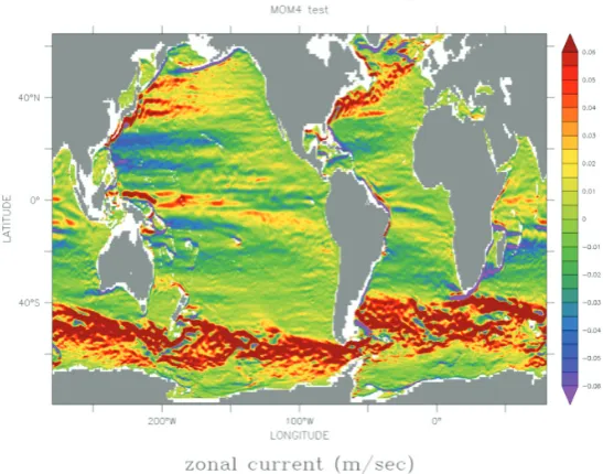
Figure 1 (page 13) shows the zonal velocity at 400m from a preliminary simulation. Space does not allow for us to compare with other simulations. Nonetheless, we note that the simulation quality is comparable to that achieved at finer resolutions, such as that described in Richards et al. (2007). We conjecture that such quality arises from the generally small lateral friction available with the Smagorinsky biharmonic scheme (Griffies and Hallberg 2000), along with the strong tracer gradients maintained with Prather (1986) advection. In addition to MOM development, GFDL ocean model developers have focused on merging features available in three ocean models: the Hallberg Isopycnal Model, the MITgcm, and MOM. This effort aims to remedy problems inherent in each model, to more rigorously test methods and parameterizations, and to optimize human resources. The resulting unified code is expected to mature during the upcoming years into a generalized vertical coordinate model with both regional and global applications.

Dedication

Throughout the history of ocean model development at GFDL, Peter Killworth has been an active participant in the community of users and developers. We sincerely thank Peter for his years of tireless service, through insightful model applications and analyses, novel algorithm designs, and super-human efforts as editor of the journal Ocean Modelling.

Bibliography

Adcroft, A., C.~Hill, and J.~Marshall, 1997: Representation of topography by shaved cells in a height coordinate ocean model, Monthly Weather Review, 125, 2293-2315.

Beckmann, A., and R.Doescher, 1997: A method for improved representation of dense water spreading over topography in geopotential-coordinate models, Journal of Physical Oceanography, 27, 581-591.

Bryan, K., A numerical method for the study of the circulation of the world ocean, 1969a: Journal of Computational Physics,

4, 347--376,

Bryan, K., Climate and the ocean circulation III, 1969b: The ocean model, Monthly Weather Review, 97, 806-824.

Bryan, K., and L.J. Lewis, 1979: A water mass model of the world ocean, Journal of Geophysical Research, 84, 2503-2517. Bryan, K., S.Manabe, and R.C. Pacanowski, 1975: A global

ocean-atmosphere climate model. Part II. The oceanic circulation, Journal of Physical Oceanography, 5, 30-46. Campin, J.-M., and H.Goosse, 1999: Parameterization of

density-driven downsloping flow for a coarse-resolution ocean model in z-coordinate, Tellus, 51A, 412-430.

Chen, D., L.Rothstein, and A.Busalacchi, 1994: A hybrid vertical mixing scheme and its application to tropical ocean models, Journal of Physical Oceanography, 24, 2156-2179.

Cox, M.D., A Primitive Equation, 1984: 3-Dimensional Model of the Ocean, NOAA/Geophysical Fluid Dynamics Laboratory, Princeton, USA.

Gent, P.R., J.Willebrand, T.J. McDougall, and J.C. McWilliams, 1995: Parameterizing eddy-induced tracer transports in ocean circulation models., Journal of Physical Oceanography,

25, 463-474.

Griffies, S.M., 1998: The Gent-McWilliams skew-flux, Journal of Physical Oceanography, 28, 831-841.

Griffies, S.M., 2004: Fundamentals of ocean climate models, Princeton University Press, Princeton, USA, 518+xxxiv pages.

Griffies, S.M., 2007: Elements of mom4p1, NOAA/Geophysical Fluid Dynamics Laboratory, Princeton, USA, 385 pp. Griffies, S.M., and R.W. Hallberg, 2000: Biharmonic friction

with a Smagorinsky viscosity for use in large-scale eddy-permitting ocean models, Monthly Weather Review, 128, 2935-2946.

Griffies, S.M., A.Gnanadesikan, R.C. Pacanowski, V.Larichev, J.K. Dukowicz, and R.D. Smith, 1998: Isoneutral diffusion in a z-coordinate ocean model, Journal of Physical Oceanography,

28, 805-830.

Griffies, S.M., R.Pacanowski, R.Schmidt, and V.Balaji, 2001: Tracer conservation with an explicit free surface method for z-coordinate ocean models, Monthly Weather Review,

129, 1081-1098.

Griffies, S.M., M.J. Harrison, R.C. Pacanowski, and A.Rosati, 2004: A Technical Guide to MOM4, NOAA/Geophysical Fluid Dynamics Laboratory, Princeton, USA, 337 pp.

Griffies, S.M., A. Gnanadesikan , K.W. Dixon , J.P. Dunne, R. Gerdes, M.J. Harrison, A. Rosati, J. Russell, B.L. Samuels, M.J. Spelman , M. Winton, and R. Zhang, 2005: Formulation of an ocean model for global climate simulations, Ocean Science, 1, 45-79.

Huang, R.X., 1993: Real freshwater flux as a natural boundary condition for the salinity balance and thermohaline circulation forced by evaporation and precipitation, Journal of Physical Oceanography, 23, 2428-2446.

Killworth, P.D., 1987: Topographic instabilities in level model OGCMs, Ocean Modelling, 75, 9-12.

ocean model, Journal of Physical Oceanography, 21, 1333-1348.

Large, W.G., J.C. McWilliams, and S.C. Doney, 1994: Oceanic vertical mixing: A review and a model with a nonlocal boundary layer parameterization, Reviews of Geophysics,

32, 363-403.

Large, W.G., G.Danabasoglu, J.C. McWilliams, P.R. Gent, and F.O. Bryan, 2001: Equatorial circulation of a global ocean climate model with anisotropic horizontal viscosity, Journal of Physical Oceanography, 31, 518-536.

Lee, H.-C., A.Rosati, and M.Spelman, 2006: Barotropic tidal mixing effects in a coupled climate model: Oceanic conditions in the northern Atlantic, Ocean Modelling, 3-4, 464-477.

Murray, R.J., 1996: Explicit generation of orthogonal grids for ocean models, Journal of Computational Physics, 126, 251-273.

Pacanowski, R.C., 1995: MOM2 Documentation, User’s Guide,

and Reference Manual, NOAA/Geophysical Fluid Dynamics Laboratory, Princeton, USA, 216 pp.

Pacanowski, R.C., and A.Gnanadesikan, 1998: Transient response in a z-level ocean model that resolves topography with partial-cells, Monthly Weather Review, 126, 3248-3270. Pacanowski, R.C., and S.M. Griffies, 1999: The MOM3 Manual,

NOAA/Geophysical Fluid Dynamics Laboratory, Princeton, USA, 680 pp.

Pacanowski, R.C., and G.Philander, 1981: Parameterization of vertical mixing in numerical models of the tropical ocean, Journal of Physical Oceanography, 11, 1442-1451.

Pacanowski, R.C., K.Dixon, and A.Rosati, 1991: The GFDL Modular Ocean Model User Guide, NOAA/Geophysical Fluid Dynamics Laboratory, Princeton, USA, 16 pp.

Prather, M., 1986: Numerical advection by conservation of second-order moments, Journal of Geophysical Research, 91, 6671-6681.

Richards, K.J., H.Sasaki, and F.Bryan, 2007: Jets and waves in the Pacific Ocean, in High-resolution numerical modelling of the atmosphere and ocean, edited by K.Hamilton and W.Ohfuchi, Springer-Verlag, New York.

Simmons, H.L., S.R. Jayne, L.C. St. Laurent, and A.J. Weaver, 2004: Tidally driven mixing in a numerical model of the ocean general circulation, Ocean Modelling, 6, 245-263. Umlauf, L., H.Burchard, and K.Bolding, 2005: GOTM: source

code and test case documentation: version 3.2, 231pp. Visbeck, M., J.C. Marshall, T.Haine, and M.Spall, 1997:

Specification of eddy transfer coefficients in coarse resolution ocean circulation models, Journal of Physical Oceanography, 27, 381-402.

Introduction

Rapid increase of computer power and significant improvement of ocean general circulation models (OGCMs) with advanced parameterizations enable us to perform long-term simulations with global high-resolution OGCMs, which represent well not only the global circulation but also pathways of narrow strong currents such as western boundary currents, frontal structures, and small scale phenomena including mesoscale eddies. The recent advent of massive parallel computer systems, including the Earth Simulator (ES) with 40 Tflops peak performance established in 2002, has opened an era of global eddy-resolving ocean simulations. We have performed a series of quasi-global simulations on the ES with a horizontal resolution of 0.1° (see below). The simulations display oceanic mean fields and variability with rich fine-scale structures, which are comparable to available observations, and intriguing results are emerging from the realistically simulated oceanic fields. The present article introduces a few examples to illustrate the great opportunity the high-resolution ocean simulations can offer to advance our understanding of ocean circulation and its variability.

Model and simulation description

OFES (OGCM for the ES) is an OGCM parallelized and highly optimized for the ES, based on MOM3 (Pacanowski and Griffies, 1999). The horizontal resolution of our quasi-global eddy-resolving model, extending from 75°S to 75°N, is 0.1° and the number of vertical levels is 54. As our first attempt, a 50-year spin-up simulation was conducted forced by monthly climatological NCEP/NCAR reanalysis fields (Masumoto et al., 2004). Surface heat fluxes are calculated using bulk formulae, and the surface salinity flux is derived from reanalysis precipitation and estimated evaporation with an additional

Sasaki, H1_{, B Taguchi}1_{, M Nonaka}2_{, Y Masumoto}2_, 3

1_{Earth Simulator Center, Japan Agency for Marine-Earth Science and Technology, Yokohama, Kanagawa, Japan.} 2_Frontier

Research Center for Global Change, Japan Agency for Marine-Earth Science and Technology, Yokohama, Kanagawa, Japan.

3_{Graduate School of Science, University of Tokyo, Tokyo, Japan.}

Corresponding author: [email protected]

A series of quasi-global eddy-resolving ocean simulations

term restoring to the monthly climatology. Following this spin-up simulation, we have performed a hindcast simulation forced by daily NCEP/NCAR reanalysis fields for the period from 1950 to 2006 (NCEP hindcast simulation, Sasaki et al., 2007). Furthermore, an additional hindcast simulation driven by the QuikSCAT satellite wind stress, provided from the J-OFURO dataset (Kutsuwada, 1998; Kubota et al., 2002), has been performed (QSCAT hindcast simulation, Sasaki et al., 2006).

50-year spin-up simulation with monthly climatological forcing

Multi-decadal hindcast simulation with NCEP reanalysis forcing

The NCEP hindcast simulation provides a long-term dataset useful to study intraseasonal to decadal variations in realistic oceanic fields. The simulated fields capture many observed features of large-scale oceanic variations on interannual to decadal time-scale such as El Niño, Indian Ocean Dipole events, Pacific Decadal Oscillation (PDO), and Pan-Atlantic Decadal Oscillation, as well as intraseasonal variations in the equatorial Pacific and Indian Oceans (Sasaki et al., 2007). Furthermore, the multi-decadal integration of the eddy-resolving model provides an unprecedented opportunity to study the low-frequency variability of narrow oceanic jets.

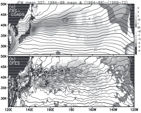
A remarkable example, in this regard, is a series of studies of decadal variation of the Kuroshio Extension (KE) front, the front associated with a swift eastward current formed after the Kuroshio separates from the Japanese coast, which has recently been recognized as an important contributor to the PDO (e.g. Schneider and Cornuelle, 2005, Qiu et al., 2007). Analyzing the OFES hindcast output, Nonaka et al. (2006) demonstrated that the observed basin-wide cooling during the early 1980s in the North Pacific (Figure 2a) was accompanied by the southward shift and intensification of the two separate oceanic fronts: the Kuroshio Extension (KE) and the subarctic/Oyashio extension fronts. They attributed the subsurface cooling along the former front and the mixed layer cooling along the latter (Figure 2b) to the southward migration of the fronts, as the associated heat flux anomalies act to damp, rather than force, the temperature anomalies (reduced heat release into the atmosphere), indicating that sea surface temperature (SST) anomalies induced by the ocean feedback to the overlying atmosphere (Tanimoto et al., 2003).

Mechanisms that cause such migration of the oceanic fronts have not been fully explored due partly to their highly chaotic, nonlinear characteristics. An EOF analysis shows that wind-forced Rossby waves explain the variation in the jet over time but predict too broad a latitudinal structure (Taguchi et al., 2007). A further analysis with meridional scale separation suggests that the large-scale component of the decadal SSH anomalies in the OFES hindcast is well reproduced by the linear baroclinic Rossby wave adjustment theory (Figure 3a and b, page 13), but a much narrower structure of the KE variability results from the internal dynamics of the jet and recirculations (Figure 3c, page 13). Interestingly the large-scale and the frontal/recirculation variability exhibit nearly identical time series, which suggests that the wind-forced Rossby waves act

as pacemaker regulating the intrinsic variability of the front (Taguchi et al., 2007).

Supplementary hindcast simulation with QuickSCAT wind stress forcing

In the QuickSCAT hindcast simulation, oceanic responses to the wind field including small scale features like the orographic wind in the lee of islands and near land boundaries are simulated well (Sasaki et al., 2006). For example, two branches of the South Equatorial Current in association with zonal band-like structures of the wind curl to the west of Galapagos Islands are realistically reproduced in OFES. Another example is the far-reaching Hawaiian Lee Countercurrent (HLCC) westward and in the lee of the Hawaiian Islands (Figure 4, page 13), for which two-way air-sea interactions are suggested to be important (Sasaki and Nonaka, 2006). In such interactions, the HLCC is further driven by the wind-stress curl induced by a warm SST band along the current, following the initial formation of the current at the Hawaiian Islands. This study demonstrates usefulness of the QuickSCAT simulation to investigate the impact of the small scale wind stress upon the ocean, which would never be possible without the fruitful combination of an eddy-resolving OGCM and satellite-observed high resolution wind forcing.

Summary and Discussion

A series of OFES simulations have been performed on the ES. The successful simulations provide us good opportunities to investigate not only mean fields but also variations with various temporal and spatial scales in the realistic simulated oceanic field including mesoscale eddies, narrow strong currents, and frontal structures, as briefly introduced in this article. We have been extending the hindcast simulations up to date. Comparison of the OFES results to recent observational data from satellite and Argo profiling floats, for example, would provide us new insights about unsolved mechanisms responsible for ocean circulations and their variability. To share with the wider research community the treasure chest from OFES, we have started opening the outputs of the spin-up simulation, as a first step (http://www2.es.jamstec.go.jp/ofes/ Figure 1. Snapshot of simulated surface current speed (m sec-1) based

on the OFES spin-up simulation

eng/). We will also open a portion of outputs from the hindcast simulation in the near future.

However, there exist some issues in the results of OFES to be solved in the near future. For example, occasional meandering of the Kuroshio south of Japan and the northwestward extent of the North Atlantic current are still unrealistic. To overcome these problems, we are trying to incorporate different parameterization schemes as well as a sea-ice model in OFES (Komori et al., 2005). Inertial mixing, tidal mixing, and non-hydrostacic processes, in addition, should be included into the future version of the high-resolution/ultra high-resolution model.

Together with the accompanying high-resolution atmospheric general circulation model (Ohfuchi et al., 2004) and the sea-ice model, a high-resolution ocean-atmosphere coupled simulation (Komori et al., 2007) is now executable on the ES, which is expected to improve predictability for high-impact phenomena with an assimilation system. Furthermore, an ocean biological model has been incorporated into OFES (Sasai et al., 2006) and will also be implemented in the coupled model in order to study predictability of marine ecosystem variability influenced by physical fields. More detailed analysis of these high-resolution models will lead us to the frontier of climate researche.

Acknowledgments

We thank members if the OFES project and the Atmosphere and Ocean Simulation Research Group in the Earth Simulator Center including Drs. W. Ohfuchi, N. Komori, and Y. Sasai. Our thanks are extended to Drs. T. Yamagata, H. Sakuma, and H. Nakamura, who contributed to the establishment of OFES project. QuikSCAT wind stress data in the J-OFURO dataset (http://dtsv.scc.u-tokai.ac.jp/j-ofuro/) are provided by Dr. K. Kutsuwada. The OFES simulations were conducted on the Earth Simulator under support of JAMSTEC.

References

Komori, N., K. Takahashi, K. Komine, T. Motoi, X. Zhang, and G. Sagawa, 2005: Description of sea-ice component of Coupled Ocean–Sea-Ice Model for the Earth Simulator (OIFES). J. Earth Simulator, 4, 31–45.

Komori, N., A. Kuwano-Yoshida, T. Enomoto, H. Sasaki, and W. Ohfuchi, 2007: High-resolution simulation of global coupled atmosphere–ocean system: Description and preliminary outcomes of CFES (CGCM for the Earth Simulator). In High Resolution Numerical Modeling of the Atmosphere and Ocean, W. Ohfuchi and K. Hamilton (Eds.), Springer, New York, in press.

Kubota, M., N. Iwasaka, S. Kizu, M. Konda, and K. Kutsuwada, 2002: Japanese ocean flux data sets with use of remote sensing observations (J-OFURO), J. Oceanogr., 58, 213–225.

Kutsuwada, K., 1998 Impact of wind/wind-stress field in the North Pacific constructed by ADEOS/ NSCAT data, J. Oceanogr., 54, 443–456.

Masumoto, Y., H. Sasaki, T. Kagimoto, N. Komori, A. Ishida, Y. Sasai, T. Miyama, T. Motoi, H. Mitsudera, K. Takahashi, H. Sakuma, and T. Yamagata, 2004: A fifty-year eddy-resolving simulation of the world ocean: preliminary outcomes of OFES (OGCM for the Earth Simulator), J. Earth Sim., 1, 35-56.

Maximenko, N., B. Bang, and H. Sasaki, 2005: Observational evidence of alternating zonal jets in the World Ocean. Geophy. Res. Lett., 32, L12607, doi:10.1029/2005GL022728. Nonaka, M., H. Nakamura, Y. Tanimoto, T. Kagimoto, and H.

Sasaki, 2006: Decadal variability in the Kuroshio-Oyashio Extension simulated in an eddy-resolving OGCM. J. Climate,

19 (10), 1970-1989.

Ohfuchi, W., H. Nakamura, M. K. Yoshioka, T. Enomoto, K. Takaya, X. Peng, S. Yamane, T. Nishimura, Y. Kurihara, and K. Ninomiya, 2004: 10-km mesh meso-scale resolving simulations of the global atmosphere on the Earth Simulator – preliminary outcomes of AFES (AGCM for the Earth Simulator). J. Earth Sim., 1, 1-34.

Pacanowski, R. C. and S. M. Griffies, 1999: The MOM 3 Manual, GFDL Ocean Group Technical Report No. 4, Princeton, NJ: NOAA/Geophysical Fluid Dynamics Laboratory, 680 pp. Qiu, B., N. Schneider, and S. Chen, 2007: Coupled decadal

variability in the North Pacific: An observationally-constrained idealized model. J. Climate, in press.

Sasai, Y., A. Ishida, Y. Yamanaka, and H. Sasaki, 2004: Chlorofluorocarbons in a global ocean eddy-resolving OGCM: Pathway and formation of Antarctic Bottom Water. Geophy. Res. Lett., 31, L12305, doi:10.1029/2004GL019895. Sasai, Y., A. Ishida, H. Sasaki, S. Kawahara, H. Uehara, and Y.

Yamanaka, 2006: A global eddy-resolving coupled physical-biological model: Physical influences on a marine ecosystem in the North Pacific, Simulation, 82 (7), 467-474.

Sasaki, H. and M. Nonaka, 2006: Far-reaching Hawaiian Lee Countercurrent driven by wind-stress curl induced by warm SST band along the current, Geophys. Res. Lett., 33, L13602, doi:10.1029/2006GL026540.

Sasaki, H., Y. Sasai, M. Nonaka, Y. Masumoto, and S. Kawahara, 2006: An eddy-resolving simulation of the quasi-global ocean driven by satellite-observed wind field: Preliminary outcomes from physical and biological fields. J. Earth Sim.,

6, 35–49.

Sasaki, H., M. Nonaka, Y. Masumoto, Y. Sasai, H. Uehara, and H. Sakuma, 2007: An eddy-resolving hindcast simulation of the quasi-global ocean from 1950 to 2003 on the Earth Simulator, In High Resolution Numerical Modeling of the Atmosphere and Ocean, W. Ohfuchi and K. Hamilton (Eds.), Springer, New York, in press.

Schneider, N. and B. D. Cornuelle, 2005: The Forcing of the Pacific Decadal Oscillation. J. Climate,18, 4355–4373. Taguchi, B., S.-P. Xie, N. Schneider, M. Nonaka, H. Sasaki, and

Y. Sasai, 2007: Decadal variability of the Kuroshio Extension:

Observations and an eddy-resolving model hindcast, J.

Climate., 20 (11), 2357-2377.

Eddy-permitting Ocean Circulation Hindcasts Of Past Decades

The DRAKKAR Group: Barnier B., Brodeau L., Le Sommer J., Molines J.-M, Penduff T., LEGI-CNRS, Grenoble, France. Theetten S., Treguier A.-M., LPO, Brest, France. Madec G., LOCEAN, Paris, France. Biastoch A., Böning C., Dengg J., IFM-GEOMAR, Kiel, Germany. Gulev S., SIO-RAS, Moscow, Russia. Bourdallé Badie R., Chanut J., Garric G., MERCA-TOR-Océan, Toulouse, France. Alderson S., Coward A., de Cuevas B., New A., NOC, Southampton, UK. Haines K., Smith G., ESSC, Reading, UK. Drijfhout S., Hazeleger W., Severijns C., KNMI, De Bilt, The Netherlands. Myers P., DEAS, Edmonton, Canada.

Corresponding author: [email protected]

1. Introduction

Research conducted by the DRAKKAR consortium is motivated by open questions related to the variability of the ocean circulation and water mass properties during past decades, and their effects on climate through the transport of heat. Of primary concern is the circulation and the daily-to-decadal variability in the North Atlantic Ocean, as driven by the atmospheric forcing, by interactions between processes of different scales, by exchanges between basins and regional circulation features of the North Atlantic (including the Nordic Seas), and by the influence of the world ocean circulation (including the Arctic). DRAKKAR carries out these investigations using a hierarchy of high resolution model configurations based on the NEMO system (Madec, 2007). Simulation outputs are carefully evaluated by comparison with collocated existing observations (Penduff et al., this issue).

The DRAKKAR consortium was created to take up the challenges of developing realistic global eddy-resolving/ permitting ocean/sea-ice models, and of building an ensemble of high resolution model hindcasts representing the ocean circulation from the 1960s to present. The Consortium favours an integration of the complementary expertise from every member of the group; the coordination of a simulation program that builds a consistent ensemble of 50 year long hindcasts; and an increase of available manpower and computer resources.

2. DRAKKAR hierarchy of models

A hierarchy of embedded model configurations of different grid resolution (from coarse to eddy-resolving) has been constructed to make possible realistic, long term (several decades) simulations of the ocean/sea-ice circulation and variability at regional and global scale, and to perform sensitivity studies investigating key dynamical processes (requiring especially high resolution) and their impact at larger scales. The DRAKKAR model configurations are used by the participating research teams to address their scientific objectives. All configurations are based on the NEMO Ocean/ Sea-Ice GCM numerical code and use the quasi-isotropic global ORCA grid (Madec, 2007).

2.1. Global ORCAii configurations

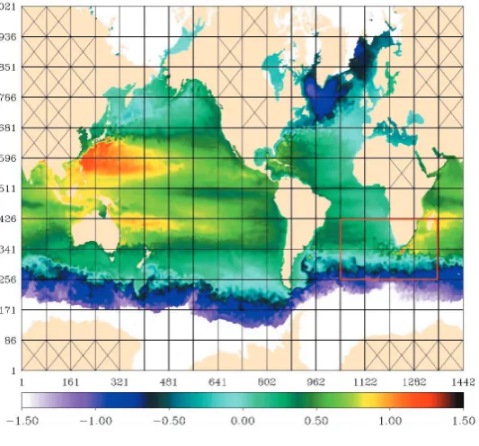
Global DRAKKAR configurations span resolutions of 2° (ORCA2), 1° (ORCA1), 1/2° (ORCA05) and 1/4° (ORCA025, Fig. 1 page 14).

The targeted configuration for the ensemble of hindcasts is the eddy permitting ORCA025, extensively described in Barnier et al. (2006). Such eddy-permitting models are still worth exploring and enhancing, since they will be the target resolution of the next generation of climate models. The ORCA grid becomes finer with increasing latitude, so the effective 1/4° resolution is 27.75 km at the equator and 13.8 km at 60°S or 60°N. It is ~7 km in the center of the Weddell and Ross Seas and ~10 km in the Arctic. In the vertical, there are 46 levels with partial steps in the lowest level. Coarser resolution configurations ORCA05, ORCA1, and ORCA2 are as similar as possible to ORCA025. The AGRIF refinement package (Debreu et al., 2007) allows local grid refinements as shown in the Agulhas Retroflection region (Fig. 1, Biastoch et al., 2007).

2.2. Regional NATLii configurations

Two North Atlantic/Nordic Seas configurations have been implemented: the 1/4° eddy-permitting NATL4 configuration (extracted from ORCA025), and the 1/12° eddy-resolving NATL12 configuration (Fig. 2). Both include prognostic sea-ice, and use open boundary conditions where information provided by the global hindcast experiments can be applied. The NATL12 resolution reaches 4.6 km at 60°N.

Fig. 2. The NATL12 domain (1615×1585×50 grid points with partial step) and the 2004-2006 mean SSH (in meter, contour interval of 0.1) from a hindcast started in 1998 (MERCATOR-Océan)

.

3. 1958-2004 global 1/4° hindcasts carried out in 2006

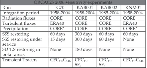
A key objective of DRAKKAR is to perform long term simulations of the atmospherically driven ocean circulation and variability over the last 50 years with the ORCA025 configuration. A coordinated series of simulations were conducted in 2006 at LEGI (G70), IFM-GEOMAR (KAB0012, KAB002) and KNMI (KNM01) (Table 1), which compare the ability of the Coordinated Ocean adn sea-ice Reference Experiment (CORE) (Large & Yeager, 2004, LY04) and ERA40 atmospheric forcing data sets, and of different T,S restoring scenarios to control the strength of the Atlantic meridional overturning cell (AMOC) and global T,S drifts.

Table 1: Forcing parametersof the different experiments. The KNM01 experiment has not been analysed yet. KAB002 is started from KAB001 on January 1st 1985.

ORCA025 2006 sensitivity experiments

Run G70 KAB001 KAB002 KNM01 Integration period 1958-2004 1958-2004 1985-2004 1958-2004 Radiation fluxes CORE CORE CORE CORE Turbulent fluxes ERA40 CORE CORE ERA40 Precipitation CORE* CORE CORE CORE* SSS restoring 60 days 300 days 60 days 60 days SSS restoring under

sea-ice 15 days 300 days 60 days None 3D T,S restoring in

polar areas None 180 days None None Transient Tracers CFC11,C14b CFC11,

SF6

CFC11,

SF6

All experiments use the downward shortwave and longwave radiation forcing from CORE (derived from satellite ISCCP products), these variables being significantly biased in ERA40 (Brodeau et al., 2006). Turbulent fluxes are calculated using LY04 bulk formulas, input variables being wind components, air temperature and air humidity. Restoring of varying strengths to climatological sea surface salinity (SSS) is also used. In addition, for the rather uncertain precipation, two different versions were used: the original CORE fields and a modified version, CORE*, in which original CORE precipation is reduced northward of 30°N by 15-20%.

3.1. Global drifts

Fig. 3 shows the global drift in temperature and sea surface height (SSH). G70 exhibits the smallest SSH drift in 47 years, partly a consequence of the restoring to SSS but also due to an excess of freshwater (and therefore volume) in the CORE data. The comparison of KAB001 and KAB002 demonstrates that this drift is more than doubled by the 3D T,S restoring applied in polar oceans in KAB001. Drifts are very comparable in G70 and KAB002 for temperature (0.001°C/y corresponding to a surface heat flux imbalance of -0.18 Wm-2), suggesting that CORE and ERA40 turbulent fluxes have similar effects on the model drift

3,54 3,55 3,56 3,57 3,58 3,59 3,6 3,61 3,62 3,63 3,64

1955 1965 1975 1985 1995 2005

-0,2 0 0,2 0,4 0,6 0,8 1 1,2 1,4 1,6

1955 1965 1975 1985 1995 2005

°C Global Me an T em per at ure meters Global me an SSH

G70 KAB001 KAB002

Fig. 3: Evolution of global ocean average temperature and sea level in G70, KAB001 and KAB002

3.2. Atlantic Meridional Overturning Circulation (AMOC) and deep overflows

The strongest AMOC is obtained with the ERA40 forcing and reduced northern hemisphere precipitation (G70), with a maximum of 17 Sv at 35N (Fig. 4). With the CORE forcing, an AMOC of similar structure and reasonable strength (above 14 Sv at 35N) is obtained only with the 3D restoring at polar latitudes (KAB001, not shown). Without this restoring, it collapses to under 12 Sv (KAB002, not shown). Other series of experiments with ORCA2, ORCA1 and ORCA05 confirmed that the AMOC obtained using original CORE turbulent fluxes and precipitation is significantly weaker than that obtained from ERA40 and reduced CORE precipitation in the northern hemisphere. Results from ORCA1 also highlight the importance of strong under-ice SSS relaxation in maintaining a strong AMOC.

Fig. 5 page 14 demonstrates that the weak 3D T,S restoring in polar seas (KAB001) maintains realistic dense overflows at the Nordic sills over the 47 years, whereas these waters rapidly disappear when this condition is removed in KAB002 (with a subsequent decrease of the AMOC). Meanwhile, the use of ERA40 turbulent fluxes instead of NCEP in the CORE data set, in combination with a modification (reduction) of the CORE precipation over the Arctic Ocean, allows a reasonable

dense water transport at the sills to be maintained without a relaxation of this kind.

Figure 4: Mean (1990-2004) AMOC in the North Atlantic for hindcast G70. Negative vaues are shaded grey and contour interval is 2 Sv. Fig. 6:

Also the freshwater balance and its effect on the deep water formation in the Labrador Sea seem to be critical in this respect. Further sensitivity experiments are underway to identify the critical model factors governing this behaviour.

3.3. Sea-ice

ORCA025 hindcasts show a decrease of the Arctic sea-ice area since the early 1980’s, as seen in satellite data. Arctic sea-ice area and concentration generally compare well with observations, in spatial patterns as well as integral values (Fig. 6, page 14). Sea-ice volume (not shown) is larger (and more realistic) in experiments using CORE turbulent fluxes (ice is too thin with ERA40). The simulation of Antarctic sea-ice is less satisfactory, with too little ice remaining in summer, and an overly large winter ice extent.

3.4. Long term variability

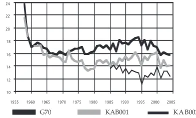
Hindcasts from the various integrations tend to simulate very comparable long term variabilities, i.e. an increase of the AMOC maximum (Fig. 7) in the 1980’s and early 1990’s and a significant decrease from the mid 1990’s. However, important year-to-year differences are observed which need to be explained.

10 12 14 16 18 20 22 24

1955 1960 1965 1970 1975 1980 1985 1990 1995 2000 2005 G70 KAB001 KA B002

Fig. 7: Variation of the AMOC maximum in the North Atlantic in hindcasts G70, KAB001 and KAB002.

24 25 26 27 28 29 30

1985 1990 1995 2000 2005

NOA A KAB001 G70

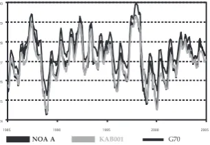
Fig. 8: Time evolution of the monthly mean ocean surface temperature (°C) in the Nino Box 3-4 in hindcasts G70, KAB001 and NOAA observations. Curve for the KAB002 run (not shown) is almost identical to KAB001.

Finally, it is obvious that applying a 3D restoring on T,S might have an impact on the simulated variability. This is illustrated in the Antarctic Circumpolar Current (ACC) transport (Fig. 9). Hindcasts without 3D restoring (G70 and KAB002) show that more than 20 years of spin-up are necessary before the ACC transport stabilises. Note that ACC transport will likely remain stronger (above 120 Sv) in KAB002 than in G70 (above 110 Sv) because of stronger winds in CORE. This spin-up phase does not exist when 3D T,S relaxation is applied at polar latitudes (beyond 50S) in KAB001. This strongly suggests that the spin-up is due to the adjustment of the mass field at high southern latitudes. The long term variability is quite different in G70 and KAB001, e.g. the latter experiment does not show the decadal oscillations typical of G70. Although weak, this relaxation tends to seriously limit the low-frequency variability.

100 110 120 130 140 150 160 170

1955 1960 1965 1970 1975 1980 1985 1990 1995 2000 2005

G70 KAB001 KAB002

Fig. 9: Mean transport (in Sv) at Drake Passage in hindcasts G70, KAB001, and KAB002.

4. Conclusion

Series of ~50-year hindcasts (of which a small part is described here) have been carried out with the DRAKKAR hierarchy of model configurations, which has allowed improvements in model numerics, parameterizations and surface forcing. The hybrid forcing using CORE radiation fluxes and precipitation fields with ERA40 turbulent variables (wind, air temperature and air humidity), referred to as the DRAKKAR Forcing Set #3 (DFS3) is currently our best choice to obtain an AMOC of realistic strength with the ORCAii configurations. Comparison of CORE and DFS3 driven hindcasts is presently under investigation and already indicates new directions for improvements for the next forcing set (DFS4) now under construction. DRAKKAR hindcasts planned for 2007 will concern the model sensitivity to sea-ice parameters and freshwater fluxes, the objective being to completely remove any restoring to SSS. Hindcasts with the eddy-resolving configuration NATL12 will also begin. The DRAKKAR hindcast database is available upon request to research scientists outside the consortium. Additional information about DRAKKAR can be found on the project web site (www.ifremer.fr/lpo/drakkar).

Acknowledgments

DRAKKAR acknowledges support for computation from the following computer centres: IDRIS in France, DKRZ and HLRS in Germany, and ECMWF for the KNMI runs. Support for DRAKKAR meetings was obtained via the French-German PICS No2475 managed by CNRS-INSU.

References

Barnier B., G. Madec, T. Penduff, J. M. Molines, A. M. Treguier, J. Le Sommer, A. Beckmann, A. Biastoch, C. Böning, J. Dengg, C. Derval, E. Durand, S. Gulev, E. Remy, C. Talandier, S. Theetten, M. Maltrud, J. McClean, and B. De Cuevas, 2006: Impact of partial steps and momentum advection schemes in a global ocean circulation model at eddy permitting resolution. Ocean Dynamics, 56: 543-567. DOI 10.1007/ s10236-006-0082-1.

Biastoch, A., C. W Böning, and Fredrick Svensson, 2007: The Agulhas System as a Key Region of the Global Oceanic Circulation, in: High Performance Computing on Vector Systems 2006, M. Resch et al. (Eds.), 163-169

Brodeau L., B. Barnier, A. M. Treguier, T. Penduff, 2006: Comparing sea surface atmospheric variables from ERA40 and CORE with a focus on global net heat flux. Flux News,

3, 6-8.

Debreu L., C. Vouland and E. Blayo, 2007: AGRIF: Adaptive

Grid Refinement in Fortran. Computers and Geosciences,

in press.

Fetterer, F., and K. Knowles. 2002, updated 2006. /Sea ice index/. Boulder, CO: National Snow and Ice Data Center. Digital media.

Large W., Yeager S. (2004) Diurnal to decadal global forcing for ocean and sea-ice models: the data sets and flux

climatologies. NCAR technical note: NCAR/TN-460+STR.

CGD division of the National Center for Atmospheric Research.

Madec G., 2007: NEMO, the ocean engine. Notes de l’IPSL, Université P. et M. Curie, B102 T15-E5, 4 place Jussieu, Paris cedex 5, En préparation.

Guoxiong Wu

Congratulations to Professor Guoxiong Wu on his election as the new President of the International Association of Meteorology and Atmospheric Sciences (IAMAS). Guoxiong is a past CLIVAR SSG member and is now a member of the Joint Scientific Committee for WCRP.

Introduction

Future climate prediction systems will include ocean models at eddy-permitting to eddy-resolving resolution, i.e. ¼° on the horizontal or finer. The development and calibration of such models requires the use of more accurate numerical schemes, and the improvement of physical subgrid-scale parameterizations for the ocean interior and its boundaries, including air-sea interactions that drive the global ocean circulation and its feedbacks to the atmosphere. The DRAKKAR consortium is developing a hierarchy of basin-scale to global ocean models (Barnier et al, this issue) to simulate and study the ocean variability driven by realistic atmospheric conditions over the last 50 years without data assimilation. These oceanic hindcasts should help understand the nonlinear interactions between fine scale processes and large-scale ocean dynamics, better interpret and take advantage of satellite and in situ observations (see Penduff et al, 2006, for an overview). However, numerical simulations require quantitative model-observation mismatch evaluations to guide dynamical studies and further model improvements, and careful dynamical assessments This paper presents an assessment method for model solutions against two complementary datasets: the ENACT-ENSEMBLES hydrographic profile database1 _{which covers the period} 1956-present and includes 7.4 million temperature/salinity (T/S) reports from hydrographic sections, moored arrays, floats, Argo and XBT observations; and the Ssalto/Duacs multimission Sea Level Anomaly (SLA) weekly maps from

altimeter measurements2 _{available since 1993. DRAKKAR}

models simulate the evolution since the late 1950’s of T, S, velocity, sea-surface height (SSH), sea-ice characteristics, and oceanic concentrations of two tracers (CFC11, 14_{C) released} in the atmosphere over that period. These variables are stored as successive 5-day averages during the integrations. Dynamical outputs are then collocated with real observations for comparison purposes. This paper focuses on the 1958-2004 global ¼° ORCA025-G70 simulation (Barnier et al, this issue), and its 2°-resolution counterpart driven by the same surface forcing.

Data preprocessing

The collocation procedure linearly interpolates model T/S fields at the geographical locations, depths, and instants when real T/S profiles were collected. Only quality-checked (unflagged) observations are considered. Model profiles are stored in the same format as observed ones to facilitate their dissemination. Colocated profiles are then processed jointly to characterize the structure of T/S model biases in space and time. Model SSH fields are interpolated as observed SLA maps, i.e. weekly and on a 1/3x1/3° Mercator grid, from 1993 to 2004. Colocated SLA databases are obtained by masking them where and when (either real or simulated) sea-ice is present, by removing at each grid point their respective 1993-1999 mean, and by removing their global spatial average every week. Lanczos filters may then be applied to split collocated SLA fields (and thus evaluate the model skill) into distinct wavenumber-frequency ranges. We focus here on the interannual SLA variability, i.e. with timescales longer than 18 months.

Assessing The Realism Of Ocean Simulations Against Hydrography And Altimetry

Penduff, T, M Juza, and B Barnier, LEGI-CNRS, BP53, 38041 Grenoble Cedex 9, France. Corresponding author: [email protected]

Upper ocean heat and salt contents

The upper ocean, which varies and interacts with the atmosphere on a wide range of time and space scales, requires a dedicated assessment in terms of heat and salt content (HC and SC). Each colour dot in Figure A (page 15) shows, for the 50-450m layer and the period 1998-2004, a collocated bias (¼° global simulation minus Argo) of HC and SC. A cold fresh bias, whose median reaches -3°C at 250m and -0.5 psu at the surface, can be seen north of the simulated North Atlantic Current. Indeed, this current progressively tends to block over the Mid-Atlantic Ridge, like in many models at this resolution, and lets cold and fresh subpolar waters invade the region off the Grand Banks. Two other shifts are revealed in the Antarctic Circumpolar Current (ACC), which locally departs from its observed route near 45° and near 90°E. Another significant T/S bias (reaching +2°C and +0.2 psu at 200m), not fully understood yet and subject to present investigations, is revealed in the Kuroshio region. The warm and salty bias visible in the northwestern Indian Ocean is due to a spurious mixing of the Red Sea overflow; our present work on bottom boundary layer parameterizations will hopefully reduce it. The DRAKKAR group is also working on improving the surface forcing function to limit the warm and salty equatorial bias seen in the tropical Indian and Atlantic basins. Over the rest of the global ocean, collocated model and Argo profiles show smaller biases after several decades of integration.

The black and green lines in Figure B (page 15) illustrate in the Sargasso Sea how Argo is being used to assess the mixed layer annual cycle simulated at ¼° resolution, in terms of monthly heat content (MLHC), depth (MLD), and temperature (MLT). The median MLHC simulated there over 1998-2004 appears overestimated between November and April, by up to a factor of 2 in winter. The lower panels show that this substantial bias is due to a winter MLD that is twice as deep as observed, and not to a warm bias (Argo and simulated MLTs are almost identical). This approach also helps evaluate hydrographic sampling errors: our results show that, in this region, Argo accurately samples the distributions (median, percentiles) of monthly MLHC, MLD and MLT: blue lines (full model) and black lines (subsampled model) are remarkably similar. Hydrographic sampling error evaluation and model observation intercomparisons are presently being extended at global scale.

Sea level interannual variability

The 2° and ¼° DRAKKAR simulations are assessed in terms of interannual SLA variability (ISV) after colocation onto altimetric maps. Because the 2° grid is re-fined meridionally to 1/3° at low latitudes, both models simulate the ISV observed there with realistic and comparable amplitudes (Figure C page 15). At higher lati-tudes, the ISV magnitude gets more realistic at ¼° resolution, especially in the eddy-active Gulf Stream (GS), North Atlantic Current and ACC (both shifted as mentioned), Kuroshio, and Agulhas region. A space-time analysis of the ISV is shown for the GS region in Figure D (page 15). SLA fields from both simulations are projected on the 1st _{EOF of the} observed ISV in this area. Its spatial structure E_o and associated

principal component P_o show that the GS latitude follows the NAO index in the real ocean with a 9-month lag (right panel). The ¼° model represents 19% of this mode’s variance, which is modest but much greater than in the 2° model (2%). Moreover, the ¼° model captures much better the delay between the NAO forcing and the GS’s response (7.8 months instead of 3.2 months at 2° resolution), yielding a better correlation with the observed ISV (0.59 instead of 0.49). Investigations of this kind are being extended to other key areas and basins of the World Ocean.

Conclusion

This quick overview of our “collocated” assessment approach has highlighted certain strengths and weaknesses of 50-year DRAKKAR simulations with respect to complementary (and recent) observations. More complete assessments are underway in other regions, depths and time ranges, and should contribute to guide model improvements. Our next multi-decadal climate-oriented simulations will be compared against the same observational databases, to precisely quantify the model sensitivities (e.g. time-mean state, various modes of variability, drifts) to thermal and mechanical surface fluxes, to resolved physical processes (e.g. mesoscale turbulence, nonlinearities, scale interactions, etc.), and to numerical choices (e.g. resolution, schemes, parameterization of non-hydrostatic, mixing or diffusive processes). These tools can also help evaluate existing or future ocean observing systems in terms of sampling errors, and strengthen the link between the observational and numerical oceanographic communities.

Ocean observations, especially prior to the recent Argo-plus-altimeter “golden age”, are both rare with respect to typical scales of motion (the Rossby radius) and dispersed in time and space. On the statistical side, model-observation mismatches can always be computed, but estimating the robustness or significance of these skills may be difficult. Besides the extension of our evaluations to various regions, times-cales, periods and depth ranges, advantage should thus progressively be also taken of complementary observational datasets (e.g. satellite SSTs, current meters, tide gauges, lagrangian trajectories, etc).

Acknowledgments

DRAKKAR-France acknowledges the computational support from IDRIS, and the support from CNES for the development of model-observation comparison methods and tools.

References

Montegut, C.D., G. Madec, A. Fischer, A. Lazar and D. Iudicone, 2004: Mixed layer depth over the Global Ocean: an examination of profile data and a profile-based climatology. J. Geophys. Res. 109, DOI: 10.1029/2004JC002378.

Penduff, T., B. Barnier, A.M. Treguier, P.Y. Le Traon, 2006 : Synergy between ocean observations and numerical simulations: CLIPPER heritage and DRAKKAR perspectives. Proceedings of the Symposium 15 Years of Progress in Radar Altimetry, Venice.

CHIME: a New Coupled Climate Model Using a Hybrid-Coordinate Ocean Component

Megann, A, A New and B Sinha, National Oceanography Centre, Southampton, UK Corresponding author: [email protected]

Introduction

The stability of the Atlantic overturning circulation under global climate change is of fundamental importance in predictions of the climate of northern Europe. However, time series from observational programmes (e.g. Bryden et al., 2005) are, so far, too short to resolve the current trends in the overturning, and results from numerical coupled models have to date been equivocal, with a wide spread of responses seen in the IPCC Fourth Assessment Report (2007). There are hints that the stability of the overturning in coupled models might be affected by the choice of the vertical coordinate of the ocean component: in the IPCC Third Assessment Report (Houghton et al, 2001) the ECHAM3/OPYC model, with an isopycnic ocean, showed the least reduction in MOC of all the models discussed there under realistic warming scenarios. In the Fourth Assessment Report the GISS-EH model, using HYCOM (essentially another isopycnic model) coupled to the GISS atmosphere model, was among the most stable of the nineteen models described, although a subsequent experiment with a similar model showed a significant reduction. It is important, therefore, to investigate in a rigorously controlled way how changing the vertical coordinate of the ocean model, while leaving other details unchanged, affects the stability of the overturning, and to understand what aspects of the coupled climate system in such models are so affected.

Here we introduce the Coupled Hadley-Isopycnic Model Experiment (CHIME). This model is identical to the Hadley Centre’s HadCM3 coupled climate model (Gordon et al., 2000), except for its use of a hybrid-coordinate ocean model (HYCOM) instead of HadCM3’s ocean model, which uses constant depth levels in the vertical. The hybrid coordinate system in HYCOM comprises constant-density layers in the ocean interior, and z-levels near the surface, and offers significant potential

advantages, such as better preservation of water masses, over a purely z-level model. We describe here an experiment using CHIME with pre-industrial atmospheric greenhouse forcing, and show that there are significant differences in ocean circulation and heat transport between the two models. We would therefore expect significant differences between predictions of the future climate from the two models.

Model description

The atmosphere and ice components of CHIME are identical to those of the control run of HadCM3. The atmospheric component is HadAM3, described fully in Gordon et al. (2000), and is on a spherical grid, with cell sizes 3.75° east-west and 2.5° north-south, and uses a hybrid vertical coordinate with 19 vertical levels. The ice model (Cattle and Crossley, 1995) is a simple thermodynamic model, with ice drift defined by the ocean surface current, and partial ice coverage allowing a representation of leads.

From Griffies et al, page 3: Ocean Modelling with MOM

Figure 1: Five year mean zonal velocity at 400m in a global 1/4 degree MOM simulation. These currents show signs of the latitudinally alternating zonal jets described by Richards et al. (2007), which were seen in a 1/10 degree simulation as well as satellite altimetre observations

From Saski et al (page 5): A series of quasi-global eddy-resolving ocean simulations

Figure 3. (a) Broad-scale component of the post (1984-1996) minus pre-shift (1968-1980) difference in OFES SSH (color shade in cm). Unfiltered OFES SSH averaged for both periods is superposed with black contours (at intervals of 10 cm). (b) Same as (a) but for SSH anomalies from the Rossby wave model (shade). (c) Same as (a) but for frontal-scale SSH (shade). Black contours designate differences in the unfiltered OFES SSH between the two periods with contour intervals of 5 cm.

Figure. 4. Annual mean current vectors at 38 m depth (m sec-1_{) and surface wind stress curl (color, unit: 10}-7 _{N m}-3_{) in 2003 based on the OFES}

Fig. 1: ORCAii global configurations. The model domain and land-sea mask are shown for the 1⁄4° ORCA025 configuration (axes correspond to grid points). Colours show a SSH snapshot (in meter) on June 24, 1998 from one of the hindcast runs (G70), sea-ice cover being in white. Boxes show the domain decomposition on a large number of processors, ocean processors (not marked by a cross, 186 of those) being the only ones retained in the calculation. On vector computers a more moderate parallelization (typically up to 32 processors) is used. The red box is the region where a 2-way grid refinement at 1/10-1/12°is being implemented.

From Barnier et al, page 8: Eddy-permitting Ocean Circulation Hindcasts of Past Decades

Figure 5: Evolution of the annual mean transport (in Sv) by density classes across the Denmark Strait. Negative values indicate a flow from the Nordic Seas into the Atlantic. The zero contour line is shown in white.

Figure A. Mixed layer heat and salt content biases from the ¼° simulation collocated with Argo profiles over 1998-2004. Each color dot quantifies a synoptic model bias.

Figure B. Top left: Local mixed layer depth (MLD) esti-mates from Argo in February (1998-2004). The MLD corresponds to a 0.2°C temperature change (Montegut et al, 2004). Other panels: Monthly mixed layer statistics (heat content in 109 _J/m2_{, depth in m, temperature in}

°C) over 1998-2004 in the Sargasso Sea from the full ¼° simulation (blue), Argo (green), and the model collocated with Argo (black). Medians (thick lines) and 17%/83% per-centiles (dashed) characterize monthly distributions.

Figure C. 1993-2004 standard deviations (cm) of observed and simulated low-frequency (LF) SLAs.

Figure D. Left: normalized 1st EOF E_o(x,y) of the observed LF SLA in the Gulf Stream region. Center: Principal com-ponent P_o(t) in cm associated with E_o (green), low-passed filtered NAO index N(t) (blue), projection of simulated SLAs on E_o (P_¼(t) in black for the ¼° model, P₂(t) in ma-genta for the 2° model). Right panel: variances of P_o, P_¼,

and P₂ scaled by the variance of P_o (line 1). Correlation of

P_o, P_¼, and P₂ with P_o (line 2). Lag between N and P_o, P_¼, P2 in months (line 3).

From Penduff et al (page 11) Assessing The Realism Of Ocean Simulations Against Hydrography And Altimetry

Figure 1: Global meridional oceanic heat transport in CHIME (red curve) and HadCM3 (green curve) in years 80-120. The other curves are from the estimates of Trenberth & Caron (2001) from the NCEP (black) and ECMWF climatologies (grey) with the errors shown dashed.

-80 -60 -40 -20 0 20 40 60 80

Latitude o_N -3

-2 -1 0 1 2 3

Tr

ansport (PW)

CHIME HadCM3

NCEP (error estimates dashed) ECMWF (error estimates dashed)

10E 20E 30E 40E 45S

40S 35S

0 3 6 9 12 15 18

10

Figure 1: Change in SST in the Northern hemisphere between the average of years 346-355 and years 11-20. The region where sea ice concentration has decreased by more than 10% is shown within the blue contour. The outcrop region for the 27.2 isopycnal (defi ned as where the isopycnal is less than 50m deep in ice free ocean) is shown within the black contour. Note non-linear scale.

Figure 3: HadGEM1 velocity fi eld on the 27.2 isopycnal (the core of the model AAIW) for years 1-10.

From Stark at al, page 18 The impact of the simulation of the Agulhas retrofl ection on the evolution of the coupled climate model HadGEM1

From Tsujino et al, Page 19: Improved representation of currents and water masses in the upper layer of the North Pacifi c Ocean in eddy-resolving OGCM

Figure 4: A forecast experiment of the oceanic state around Japan. Left panels: forecast. Right panels: real state estimated by data assimilation. Shade and vector is temperature and velocity at 100 m depth, respectively. The prediction begins on 1 July 2004 with an initial condition obtained from the data assimilation. The evolution of the oceanic state is shown by the interval of 30 days. This case is the development of the Kuroshio large meander, which is the sole large meander event since 1990.

From Piggot et al, page 21:Multi-scale ocean modelling with adapting unstructured grids

Figure 1: Section of unstructured mesh generated for the North Atlantic. The representation of the bathymetry and coastlines has been optimised using Terreno (Gorman et al., 2006). Regions of high curvature, such as the mid-Atlantic ridge and Celtic shelf break make use of increased anisotropic resolution.

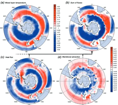
Figure. 2 Heat budget analysis: M _{o p}N M M _MLD

z T u y T v x T u MLD

CQ

t T

� � � � � � � � � �

� �

) (

� where TM _{is the mixed layer temperature, Q}

N is the net surface heat

fl ux, Cp is the specifi c heat capacity of seawater, t0 is a reference

density and MLD is the monthly mean mixed layer depth. Panels show regressions on SAM index of (a) mixed layer temperature (o_C);

(b) sum of mixed layer heat budget terms (o_Cs-1_{); (c) net surface heat}

fl ux term (o_Cs-1_{) and (d) meridional heat advection term (}o_Cs-1_{). Colour}

scaling is identical in panels (b)-(d)