This is a repository copy of
Modelling Canopy Flows over Complex Terrain
.
White Rose Research Online URL for this paper:
http://eprints.whiterose.ac.uk/100409/
Version: Accepted Version
Article:
Grant, ER, Ross, AN orcid.org/0000-0002-8631-3512 and Gardiner, BA (2016) Modelling
Canopy Flows over Complex Terrain. Boundary-Layer Meteorology, 161 (3). pp. 417-437.
ISSN 0006-8314
https://doi.org/10.1007/s10546-016-0176-3
© 2016 Springer Science+Business Media Dordrecht. This is an author produced version
of a paper published in Boundary-Layer Meteorol. The final publication is available at
Springer via http://dx.doi.org/10.1007/s10546-016-0176-3. Uploaded in accordance with
the publisher's self-archiving policy.
[email protected] https://eprints.whiterose.ac.uk/
Reuse
Unless indicated otherwise, fulltext items are protected by copyright with all rights reserved. The copyright exception in section 29 of the Copyright, Designs and Patents Act 1988 allows the making of a single copy solely for the purpose of non-commercial research or private study within the limits of fair dealing. The publisher or other rights-holder may allow further reproduction and re-use of this version - refer to the White Rose Research Online record for this item. Where records identify the publisher as the copyright holder, users can verify any specific terms of use on the publisher’s website.
Takedown
If you consider content in White Rose Research Online to be in breach of UK law, please notify us by
(will be inserted by the editor)
Modelling canopy flows over complex terrain
1Eleanor R. Grant · Andrew N. Ross · Barry A. 2
Gardiner 3
4
Draft: 31st July 2015
5
Abstract Recent studies of flow over forested hills have been motivated by a num-6
ber of important applications including understanding CO2and other gaseous fluxes
7
over forests in complex terrain, predicting wind damage from trees and modelling
8
wind energy potential at forested sites. Current modelling studies have focused
al-9
most exclusively on highly idealised, and usually fully forested, hills. This paper
10
presents model results for a site on the Isle of Arran, Scotland with complex terrain
11
and a heterogeneous forest canopy. The model uses an explicit representation of the
12
E. R. Grant
Institute for Climate and Atmospheric Science, School of Earth and Environment, Univ. of Leeds, UK.
Present address: British Antarctic Survey, High Cross, Madingley Road, Cambridge, CB3 0ET, UK
A. N. Ross
Institute for Climate and Atmospheric Science, School of Earth and Environment, Univ. of Leeds, UK.
B. A. Gardiner
Forest Research, Northern Research Station, Roslin, Midlothian EH25 9SY, Scotland. Present address:
INRA, UMR 1391 ISPA, 33140 Villenave D’Ornon and Bordeaux Sciences Agro, UMR 1391 ISPA, 33170
canopy and a one-and-a-half order turbulence closure for the turbulence within and
13
above the canopy. The validity of the turbulence closure scheme is assessed using
14
the turbulence data from the field experiment before comparing predictions of the
15
full model with the field observations. For near-neutral stability the results compare
16
well with the observations showing that a relatively simple canopy model such as this
17
can accurately reproduce the flow patterns observed with complex terrain and
realis-18
tic variable forest cover, while at the same time remaining computationally feasible
19
for real case studies. The model allows a closer examination of the flow separation
20
observed over complex forested terrain. Comparison with model simulations using a
21
roughness length parametrization show significant differences, particularly with
re-22
spect to flow separation and this highlights the need to explicitly model the forest
23
canopy if detailed predictions of the near-surface flow around forests are required.
24
Keywords Complex terrain, First order mixing length closure, Flow separation, 25
Forest canopy, Numerical modelling
26
1 Introduction 27
There has been significant interest over the last few years in modelling the effects
28
of canopy flow over complex terrain. This has been motivated by a number of
is-29
sues, particularly the need to understand and interpret CO2flux measurements over
30
complex forested sites, where advective affects can lead to a significant difference
31
between above-canopy fluxes and the source / sinks within the canopy (Katul et al.,
32
2006; Ross and Harman, 2015). Other important applications include assessing wind
33
damage to trees and estimating potential wind energy resources for wind farms.
world sites tend to be complicated, in terms of both the terrain and heterogeneity in
35
the forest canopy. In contrast the vast majority of modelling studies so far have
ad-36
dressed highly idealised problems. Many concentrate on flat, homogeneous canopies
37
(e.g. Pinard and Wilson, 2001). Where they do study heterogeneous problems, these
38
are often highly idealised such as a sharp forest edge (Liu et al., 1996; Yang et al.,
39
2006; Dupont and Brunet, 2008, 2009; Dupont et al., 2011; Banerjee et al., 2013;
40
Schlegel et al., 2015) or idealised fully forested hills (Ross and Vosper, 2005; Ross,
41
2008; Dupont et al., 2008; Patton and Katul, 2009). The recent paper of Ross and
42
Baker (2013) takes this slightly further by looking at partially forested (but still
ide-43
alised) hills. There are good reasons for starting with such idealised problems. It
44
allows for a systematic study of the individual processes influencing flow over
for-45
est hills. These problems may also be amenable to analytical analysis (e.g. Finnigan
46
and Belcher, 2004). It is also possible to reproduce some of these problems in the
47
laboratory (e.g. Poggi and Katul, 2007) to provide validation data for the models.
48
However, ultimately we need to be able to model flow over real, complex terrain with
49
complicated, heterogeneous forest cover. This study aims to do that. The simulations
50
discussed here are based on the field experiment described in Grant et al. (2015) and
51
the field observations will be used to validate the modelling. The aim is to assess the
52
feasibility of using existing models to tackle such complex problems and to
investi-53
gate some of the issues faced when making such realistic simulations.
54
There are currently two principal approaches used for modelling turbulence in
55
canopy flows: mixing length closure schemes (e.g. Pinard and Wilson, 2001; Ross and
56
Vosper, 2005; Banerjee et al., 2013) and large-eddy simulations (LES) (e.g. Brown
et al., 2001; Yang et al., 2006; Ross, 2008; Dupont et al., 2008; Patton and Katul,
58
2009). LES offers advantages in terms of requiring fewer assumptions about the
na-59
ture of the turbulence in forest canopies, but the excessive computational demands
60
make it usually impractical in terms of modelling realistic cases over large domains,
61
although Schlegel et al. (2015) have demonstrated that this is possible, at least for
62
idealised flow across a forest edge with a real heterogeneous canopy structure.
Pre-63
vious work has shown that while there are limitations in its applicability, mixing
64
length closure schemes actually perform reasonably well in terms of predicting mean
65
flow over relatively flat, homogeneous canopies from both a theoretical (Finnigan
66
and Belcher, 2004) and a practical (Pinard and Wilson, 2001) perspective. In a recent
67
paper Finnigan et al. (2015) have reviewed the applicability and limitations of mixing
68
length closure schemes from a theoretical perspective. In this study we will look at
69
how applicable such schemes are for modelling more complex terrain and
heteroge-70
neous forest canopies in reality, using the one-and-a-half order mixing length closure
71
scheme from Ross and Vosper (2005).
72
In section 2 the model setup is described. Section 3 provides some validation
73
for the mixing length closure by testing the closure assumptions using observational
74
data over complex terrain from Grant et al. (2015). Section 4 presents a comparison
75
of the model and observational results in terms of the mean flow, momentum fluxes
76
and turbulent kinetic energy. The sensitivity of the model to the parametrization of the
77
surface is investigated in Section 5, and the model results are used to better understand
78
the complicated flow separation over a realistic site. Finally section 6 provides some
79
discussion and conclusions.
2 Description of observations and model 81
The case study used in this paper comes from a field experiment conducted on the
82
Isle of Arran, Scotland during spring 2007. The experiment is described in detail
83
in Grant et al. (2015). The field site is the ridge Leac Gharbh which is situated on
84
the north-east coast of Arran. The ridge is orientated north-west / south-east with
85
the southern end of the ridge being mostly covered with Sitka spruce and mixed
de-86
ciduous trees. Here we make use of wind speed and direction measurements made
87
from a network of 12 automatic weather stations (AWS) and 3 instrumented towers
88
as described in Grant et al. (2015). The AWS were fitted with cup anemometers and
89
wind vanes at 2m height and were located both within and outside the forest canopy.
90
The 3 towers varied in height from 15 to 23 m with 4 sonic anemometers mounted
91
on each. The towers formed a transect across the forested part of the ridge. The data
92
presented is based on 15-minute average wind speeds and directions. The choice of
93
coordinate system for sonic anemometer measurements in complex, forested terrain
94
is non-trivial, as highlighted by a number of recent studies including Ross and Grant
95
(2015); Oldroyd et al. (2015), however for simplicity and for consistency in
compar-96
ing with the model, a double rotation into streamwise coordinates is carried out here,
97
as in Grant et al. (2015). This coordinate system means u is the velocity component
98
in the streamwise direction, w is the slope normal velocity component and v is the
99
remaining velocity component in the axis perpendicular to u and w.
100
Given the uncertainty in the forest parameters and in the upstream flow
condi-101
tions, and also the local variability in the observations, this study aims to model some
102
generic flow conditions (neutral flow with a 10 m s−1geostrophic wind and different
fixed geostrophic wind directions) and compare them with the observational
clima-104
tology, rather than trying to precisely model particular case studies. The focus here
105
is on near-neutral flow for a couple of reasons. Firstly, much of the previous
theoret-106
ical work (e.g. Finnigan and Belcher, 2004; Ross and Vosper, 2005; Ross and Baker,
107
2013) is for neutral flow, and one motivation of the paper is to test how these ideas
108
can be applied to more complex terrain and canopy cover. Secondly, under stable
109
conditions canopy flows are known to decouple, with an in-canopy drainage flow
dis-110
tinct from the above canopy flow (see e.g. Belcher et al., 2012). This is an important
111
problem, but the mixing length closure model described here has not been developed
112
or tested with such flows in mind, and so for this study such regimes are excluded.
113
Numerical simulations were conducted using the BLASIUS model, originally
de-114
veloped at the UK Met Office and described in Wood and Mason (1993). The model
115
solves the three-dimensional, time-dependent Boussinesq equations of motion in a
116
terrain-following coordinate system. The addition of a canopy drag term and a
mod-117
ified turbulence scheme (see Ross and Vosper, 2005) make it suitable for modelling
118
canopy flows over hills. It has been used for studying a range of idealised problems
119
related to canopy-covered hills (Brown et al., 2001; Ross and Vosper, 2005; Ross,
120
2008, 2011; Ross and Harman, 2015), partially forested hills (Ross and Baker, 2013)
121
and variable canopy densities (Ross, 2012). The model has been validated against
122
wind tunnel measurements over a hill, and against observations from a flat
hetero-123
geneous forest (Ross and Vosper, 2005), but this is the first time the model has been
124
applied to such complex, heterogeneous terrain as this.
The simulations described here use a one-and-a-half order mixing length closure
126
scheme with a prognostic equation for the turbulent kinetic energy, k. The scheme
127
is described in Ross and Vosper (2005), however in summary the eddy viscosity is
128
calculated asνt=Γ1/20 k1/2lm whereΓ0is the (assumed constant) ratio between the
129
stress and the energy and lmis the mixing length, which is constant within the canopy
130
and scales with height above the canopy. In BLASIUS a default value ofΓ0=0.357
131
is used. The turbulent kinetic energy satisfies
132
ρDk
Dt =ρ∇·(νt∇k) +τi j
∂Ui
∂xj
−ρε (1)
whereρis the density of the air, Uiis the mean wind speed,τi jis the Reynolds stress
133
tensor andεis the dissipation. The Reynolds stress is modelled asτi j≡ −ρu′iu′j =
134
ρνtSi jwhere Si j=∂Ui/∂xj+∂Uj/∂xiis the deformation tensor. To close the
prog-135
nostic equation for turbulent kinetic energy requires the dissipation term, εto be
136
parametrized. This takes the standard form above the canopy (εcc=k3/2Γ3/20 /lm),
137
with an enhanced dissipation εf d =Ca|U|k within the canopy (following Wilson
138
et al., 1998) to account for canopy drag rapidly converting energy from large scales
139
to small, quickly dissipated “wake scales”. The overall dissipation within the canopy
140
is taken as the maximum of these two termsε=max(εcc,εf d). See also Katul et al.
141
(2004) for a useful discussion of k and k−εmodels applied to canopy flows.
142
Terrain and land use data (50 m horizontal resolution) came from the Ordnance
143
Survey Landranger and MasterMap products, accessed via EDINA (2011). The model
144
domain was 6 km×6 km with 120 grid points in each direction giving a horizontal
145
resolution of 50 m. The domain is centred on the Leac Gharbh ridge. The height of
146
the domain was 5 km with a stretched vertical grid of 80 points giving a vertical
T1T2T3
x(km)
0 1 2 3 4 5
y
(k
m
)
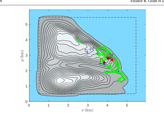
[image:9.595.72.405.70.302.2]0 1 2 3 4 5
Fig. 1 The model domain used in the BLASIUS simulations. The shaded grey colour denotes the terrain
height, with contours every 25m. The solid green line marks the boundary of the forest. The red circles
labelled T1-T3 denote the 3 instrument towers and the blue + show the location of the AWS. The light blue
area around the edges denotes sea, where a lower roughness length z0is used. The dashed line marks the
edge of the damping layer.
olution varying from 0.5 m at the surface to approximately 180 m at the top of the
148
domain. In order to keep the model domain to a computationally manageable size
149
lateral periodic boundary conditions were used, with a damping layer applied over
150
the outermost 500m of the domain to relax the solution back towards the geostrophic
151
wind profile. The terrain is also smoothed to zero in the damping layer domain and
152
the surface roughness set to the value over the sea to ensure continuity across the
153
periodic boundaries. Figure 1 shows the model domain and illustrates the topography
154
and forest cover used. The white area around the edges and to the top right is sea.
The location of regions of different land use is accurately obtained from the
Ord-156
nance Survey data, however there is significant uncertainty in the correct roughness
157
length and canopy parameters to use in these regions. Field measurements of tree
158
properties made by Forest Research near the field site (Grant et al., 2015) suggest that
159
a canopy height h=15 m, uniform canopy density of 0.5 m2m−3and canopy drag
co-160
efficient Cd=0.25 are broadly representative of the forest cover on the ridge. There
161
is variation in the canopy cover, however given the lack of detailed measurements
162
across the whole ridge and the other uncertainties in the modelling, these
represen-163
tative canopy parameters should be reasonable. The roughness length used over the
164
land outside the forest and at the forest canopy floor is 0.05 m, representative of
grass-165
land. Over the sea a lower representative value of 0.005 m is used. The sensitivity of
166
the results to these roughness lengths will be assessed later. The model simulations
167
were all run to steady state (approx 1000 s or twice the domain advection time).
168
3 Validation of mixing length closure 169
Typically turbulence closure schemes are validated using data from relatively flat,
170
homogeneous sites (e.g. Pinard and Wilson, 2001). To test the validity of the
tur-171
bulence closure assumptions in BLASIUS over a site with complex, heterogeneous
172
terrain observational data from the field campaign described in Grant et al. (2015)
173
is analysed. The one-and-a-half order turbulence scheme in BLASIUS assumes that
174
the Reynolds stress tensorτi j is given byτi j=−ρu′iu′j=ρνtSi j. Even in complex
175
canopy flows scaling analysis suggests that the stress tensor Si jis usually dominated
176
by the vertical gradients of the horizontal velocity components, and so here we focus
−5
0
5
10
−2
0
2
4
6
a) − u ′w ′(m 2s − 2)T1
−5
0
5
10
−2
0
2
4
6
b)T2
−5
0
5
10
−2
0
2
4
6
c)T3
−5
0
5
10
−2
0
2
4
6
d) − u ′w ′(m 2s − 2)−5
0
5
10
−2
0
2
4
6
e)−5
0
5
10
−2
0
2
4
6
f)−5
0
5
10
−2
0
2
4
6
g) − u ′w ′(m 2s − 2)−5
0
5
10
−2
0
2
4
6
h)−5
0
5
10
−2
0
2
4
6
i)−5
0
5
10
−2
0
2
4
6
j) − u ′w ′(m 2s − 2)k1/2du/dz(m s−2)
−5
0
5
10
−2
0
2
4
6
k)k1/2du/dz(m s−2)
−5
0
5
10
−2
0
2
4
6
l)k1/2du/dz(m s−2)
Wind direction (
° )
[image:11.595.75.414.74.535.2]100 200 300
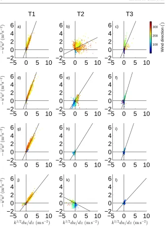
Fig. 2 Momentum flux u′w′in streamwise coordinates as a function of k1/2∂u/∂z where k is the turbulent
kinetic energy. The colours denote the direction of the mean wind for each 15-minute averaged data point.
The solid line is a best fit line to the data which passes through the origin. The slope of the line is
pro-portional to the mixing length lm. The three columns correspond to towers T1 (left), T2 (centre) and T3
(right). The rows correspond to the different heights on each tower with the top row corresponding to the
−5
0
5
10
−2
0
2
4
6
a) − v ′w ′(m 2 s − 2 )T1
−5
0
5
10
−2
0
2
4
6
b)T2
−5
0
5
10
−2
0
2
4
6
c)T3
−5
0
5
10
−2
0
2
4
6
d) − v ′w ′(m 2s − 2)−5
0
5
10
−2
0
2
4
6
e)−5
0
5
10
−2
0
2
4
6
f)−5
0
5
10
−2
0
2
4
6
g) − v ′w ′(m 2 s − 2 )−5
0
5
10
−2
0
2
4
6
h)−5
0
5
10
−2
0
2
4
6
i)−5
0
5
10
−2
0
2
4
6
j) − v ′w ′(m 2 s − 2 )k1/2dv/dz(m s−2)
−5
0
5
10
−2
0
2
4
6
k)k1/2dv/dz(m s−2)
−5
0
5
10
−2
0
2
4
6
l)k1/2dv/dz(m s−2)
Wind direction (
° )
[image:12.595.73.411.74.530.2]100 200 300
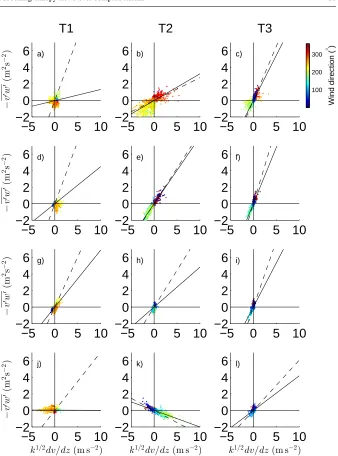
Fig. 3 As for Fig 2, but for v′w′as a function of k1/2∂v/∂z. The dotted line shows the slope of the equivalent
on−u′w′≈Γ1/2
0 lmk1/2∂u/∂z and−v′w′ ≈Γ 1/2
0 lmk1/2∂v/∂z. The vertical gradients
178
in streamwise coordinate are calculated by first rotating into a fixed frame of
refer-179
ence relative to the ground, calculating the gradients at the midpoints between the
180
observations by finite differencing, linearly interpolating the results back onto the
181
measurement heights and then finally rotating back into the local streamwise
coordi-182
nates at each height. Here quality controlled data from Grant et al. (2015) for all wind
183
directions and stabilities is used to assess the validity of the closure assumptions. The
184
quality control involves ensuring sufficient data is available in each 15-minute
aver-185
aging period and also that the data passes the stationarity test of Foken and Wichura
186
(1996) as described in Grant et al. (2015). This quality controlled data amounts to
187
about 4000 data points for T1, 3600 data points for T2 and 2500 data points for T3.
[image:13.595.53.418.60.675.2]188
Figure 2 shows the momentum flux,−u′w′, plotted against k1/2du/dz for the 3
189
turbulence towers (T1, T2 and T3) situated across the ridge. The linear best fit line
190
through the data is also plotted. The slope of this line is proportional to the average
191
mixing length, lmwith the constant of proportionality beingΓ1/20 . The results show
192
that for tower T1 the data collapses well, with the mixing length relatively constant
193
with height within the canopy (the best fit line has the same slope at different heights).
194
There is some slight evidence of a decreased mixing length at the lowest height due
195
to the close proximity to the ground. Similar plots of v′w′against k1/2dv/dz in Fig. 3
196
show a relatively small vertical flux of across-stream momentum, suggesting little
197
directional shear and an approximately two-dimensional flow.
198
In contrast to tower T1, at tower T2, which is surrounded on nearly all sides by
199
trees and where there is often flow separation at the lower two levels, the collapse of
the data is far less good. The fluxes are generally lower, and there is significant
direc-201
tional wind shear in the vertical (see Grant et al., 2015, for details). This directional
202
shear is not observed at tower T1 and may be responsible for the poorer data collapse
203
at tower T2. Interestingly there does seem to be a dependence on the mean wind
di-204
rection, which is most noticeable at the top of T2. For particular wind directions (e.g.
205
easterly winds) the data does seem to collapse, but the slope is a function of the wind
206
direction. For other wind directions (e.g northerly / north-westerly winds) there is
207
no clear collapse. This may suggest that the mixing length is dependent on the flow
208
direction. This would makes sense since it is the upwind forest canopy density which
209
will control the observed mixing length. At the second height down on T2 there is
210
a much stronger linear relationship, but the sign of the flux exhibits a strong
depen-211
dence on the wind direction. The negative values of u′w′are at first glance surprising
212
given the wind speed typically increases with height at this location. Due to the strong
213
direction wind shear however du/dz is actually negative. It is not clear why the data
214
collapse is better at the second height down than at the top of T1, although it might be
215
related to the proximity of the top of the tower to canopy top, or to difficulties in
accu-216
rately calculating the shear in this region. The strong directional wind shear at the the
217
second height down might also result in a stronger correlation between the local shear
218
and the local turbulent momentum fluxes. A further complication is the presence of a
219
SW-NE aligned fire break across the ridge just to the south of T2 which may impact
220
on the flow for certain wind directions. It is not clear though that the data collapse
221
is worse for cases where the wind is blowing from this direction. At the lowest two
222
measurement heights, in the region of separated flow and where the speeds are
est, there is little evidence of any linear relationship between u′w′and k1/2du/dz. At
224
the lowest height, the apparent trend is negative, which is contrary to the underlying
225
assumptions in the closure model and suggests either a non-local source for the
tur-226
bulent eddies responsible for the momentum transport or errors in the calculation of
227
the wind shear at this location. The scatter however is large and so the relationship is
228
not clear. The plots of v′w′against dv/dz show that the cross-stream momentum flux
229
is not insignificant at this site (again, consistent with the importance of directional
230
shear). The first order closure still seems to hold reasonably well, particularly at the
231
second height from the top of the mast. The slopes of the solid and dashed lines are
232
very similar showing that the mixing lengths inferred from v′w′ are very similar to
233
those derived from u′w′, which is again encouraging. At the lowest height, as for u′w′,
234
the data collapses surprisingly well but gives a negative slope. The other noticeable
235
feature at tower T2 is that the sign of the shear term k1/2dv/dz is strongly dependent
236
on wind direction suggesting two different flow regimes for broadly north-easterly
237
and broadly south-westerly flow, which is again consistent with the profiles given in
238
Grant et al. (2015) and with the plots of k1/2du/dz.
239
T3 is taller that T1 and T2, and so the top measurements are above the canopy.
240
Despite this the data collapse is less clear. For much of the time and for certain wind
241
directions the data does lie on a straight line, however again during periods of flow
242
separation there is often a positive value of u′w′, indicative of the effects of
direc-243
tional shear. The diagnosed mixing lengths are relatively constant with height, similar
244
to those at tower T1. The plots of v′w′show a similar collapse of the data to those of
245
u′w′and very similar mixing lengths. Values of v′w′lie somewhere between those at
towers T1 and T2, suggesting that direction shear may be important here, but
proba-247
bly less than at tower T2. The data at the lower heights collapses well, but as for u′w′
248
there is a directional dependence on the mixing length at the top of the tower.
249
Calculating an average mixing length from the slope of the best-fit line using only
250
data with u′w′<0 gives fairly consistent results, with mixing lengths in the range of
251
2.3−3 m at most heights on towers T1 and T3, and lower values close to 1.5 m at
252
the lowest instrument heights. These mixing length values are surprising consistent
253
with values derived from the plots of v′w′, particularly at towers T2 and T3 where
254
the directional shear and cross-stream momentum flux are most important. The data
255
from the top of tower T3 remains somewhat different and is separated into two flow
256
regimes. The bulk of the data, for broadly easterly winds with no flow separation, lies
257
on the steeper line with a slope giving lm≈4.8 m. This tower is taller than towers T1
258
and T2 and the instrument is well above the height of the canopy, so one would expect
259
to see an increase in the mixing length at this location under these conditions. The
260
remaining data is predominantly for westerly cases with flow separation and stronger
261
directional shear and is characterised by larger values of the shear term k1/2du/dz but
262
weaker momentum fluxes. Mixing length closure schemes are known to have issues
263
in separated flows (e.g. Ross et al., 2004) and so it is perhaps not surprising that a
264
different behaviour is observed in this separated flow regime.
265
From all these profiles one can conclude that in many cases (particularly where
266
there is little directional shear) a mixing length closure assumption is reasonable,
267
and that the diagnosed mixing lengths from the observations are consistent with the
268
common assumptions of a constant mixing length in the canopy. Only at T3 do
surements extend much above the canopy, and these seem to suggest a mixing length
270
which increases with height (at least for non-separated flow), although there are not
271
enough measurements to conclude whether this relationship is linear with height as
272
expected from theory. This has important implications for the numerical modelling
273
of canopy flows in complex terrain. There remain a number of cases (particularly at
274
T2 near the summit) where there is flow separation and strong directional shear, and
275
in these cases the mixing length closure assumptions do not appear to hold as well.
276
Some cases with directional shear (e.g. the 2nd height from the top on tower T2) do
277
actually support the assumption of a constant mixing length, and so it may be that it is
278
not the directional shear per se which is important, but the fact that the mixing length
279
is strongly dependent on the wind direction due to very different upstream conditions
280
in different directions. For many of the cases where the simple mixing length closure
281
assumptions do not hold the corresponding momentum fluxes are small anyway, and
282
so the overall impact on the mean flow may not be significant. There is also more
283
uncertainty associated with the observations in the cases with significant directional
284
shear. Weak mean flow and larger directional shear make it harder to calculate the
285
gradient terms du/dz in the mean flow in a robust manner. Weak mean winds also
286
lead to more variability in the calculated streamwise coordinate rotations, which may
287
impact on the calculated momentum fluxes. Both of these are likely to increase the
288
scatter in the results as for example is observed in the plots of u′w′ from the lower
289
two instruments on T2 (Figs. 2(h) and (k)) located deep within the canopy.
Over-290
all these results support the use of the one-and-a-half order mixing length closure
291
scheme implemented in the BLASIUS model. The precise impact the regions of
rectional shear, and the associated errors in the mixing length turbulence closure,
293
have on model predictions of mean flow fields will be investigated in the following
294
section by comparing results from the full model with the observations.
295
4 Comparison of model and observations 296
As in Grant et al. (2015), only observational data from near-neutral or
transition-to-297
stable conditions is used in order to allow comparison with the neutral flow model
298
simulations. Two flow regimes of north-easterly and south-westerly are presented
299
here. These are the same cases used in Grant et al. (2015), where a detailed
obser-300
vational analysis of these cases is given. There are some issues with interpreting cup
301
anemometer measurements, particularly in a canopy flow. Firstly, the cup
anemome-302
ters have a stall speed (notionally 0.7 m s−1in this case) below which they will not
303
turn, and so under low wind conditions (typical in the canopy) they will tend to give
304
an underestimate of the wind speed compared to sonic anemometer measurements.
305
Secondly, at higher wind speeds, the cup will respond both to the mean wind, but
306
also to larger turbulent gusts, and will therefore tend to overestimate the wind speed
307
so the measured wind speed is effectivelypU2+2k
[image:18.595.51.416.211.648.2]308
Figure 4 shows wind roses from the 12 AWS and 3 tower sites for both
observa-309
tional and model data. The observations are for cases where the wind is broadly
north-310
easterly with the wind direction at AWS ARP (a ridge top site outside the canopy)
311
being between 50◦and 90◦. This equates to about 15 hours of data. The model results
312
are for a geostrophic wind direction of 90◦, which gives a 2m wind direction at AWS
313
ARP of about 80◦. Figure 4(a) show wind roses of 15-minute averaged winds from
the 15 hours of observational data, while Fig. 4(b) shows the equivalent wind rose plot
315
from the model, with just a single wind value at each location. Note the model is for
316
a representative geostrophic wind speed of 10 m s−1. This gives winds at the AWSs
317
which are similar in magnitude to the observations, but the values cannot be directly
318
compared. It is worth noting that the red bins are for mean winds which are close to or
319
below the stall speed of the cup anemometers on the AWS and so the precise values
320
should be treated with some caution. It is likely that these are under-representing the
321
true wind speed due to stalling.
322
It is however interesting to look at the wind directions and the variations in wind
323
speed across the hill for both the observations and model. In the easterly case there
324
is evidence of flow separation in the observations from a number of the AWS sites
325
(Fig. 4a), with sites within the canopy on the ridge and over the lee slope showing
326
strong deviations from the geostrophic wind. The flow is generally not reversed, but
327
there can be significant variability in wind direction. Outside the canopy there is less
328
variability in wind direction with winds predominantly remaining north-easterly. As
329
might be expected, wind speeds outside the canopy are also higher than those in the
330
canopy. The tower profiles (Fig. 4c) show little sign of separation, with tower T1 (on
331
the lee slope) still showing broadly north-easterly winds, except at the lowest level in
332
the canopy where there is some indication of more south-easterly winds. This appears
333
to be a marginal case of flow separation and highlights how three-dimensional flow
334
separation can be over real terrain, in contrast to previous idealised two-dimensional
335
studies. In this case the model predictions broadly agree with the observations.
Out-336
side the canopy the predicted flow is easterly / north-easterly and stronger than inside
the canopy (Fig. 4b). Over the upwind slope the flow remains north-easterly, while
338
near the ridge the wind is more along the ridge. The two AWS sites near the forest
339
edge on the lee slope (ARA and ARC) show light winds and complete flow reversal.
340
This is rather more dramatic than the observations, and may reflect the fact that
unre-341
solved small scale local features are important in determining wind direction in very
342
light winds and under an adverse pressure gradient. The observations are particularly
343
variable at these sites. The model tower profiles (Fig. 4d) also look very similar to
344
the observations, and even show the same tendency for the flow to become
south-345
easterly at the lowest level on tower T1. The model also shows a similar (though less
346
pronounced) tendency for the wind to turn clockwise at lower levels on tower T2,
347
which is not seen in the observations. This tower is close to the summit of the ridge
348
and so the precise wind direction is likely to be quite sensitive to the exact location of
349
the grid point. In both observations and model, the results at tower T3 on the upwind
350
slope show a north-easterly wind at all levels. Broadly there is agreement between
351
the model and observations in terms of the wind speeds. The highest winds are seen
352
above the canopy, particularly at the top of tower T2 near the ridge summit. The
low-353
est winds in the observations are at the lower levels on towers T1 and T2. The model
354
is slightly different, with low wind speeds low down on tower T1, but slightly higher
355
winds at the bottom of tower T2. Again the differences here perhaps represent the
356
sensitivity of the exact grid location at the ridge top.
357
Figure 5 is similar to Fig. 4, except that results are for broadly south-westerly
358
winds (observed wind directions in the range 240◦to 260◦- about 50 hours of data).
359
The model results are for a westerly geostrophic wind (corresponding to a wind
x(m) y (m ) a) ARA ARB ARC ARE ARF ARG ARH ARJ ARL ARN ARP ARQ
0 400 800 1200 1600 2000
0 400 800 1200 1600 2000 x(m) y (m ) b) ARA ARB ARC ARE ARF ARG ARH ARJ ARL ARN ARP ARQ
0 400 800 1200 1600 2000
0 400 800 1200 1600 2000
wind speed (m s
−1 ) 0 1 2 3 4 5 6 10 15
T1 T2 T3
0 5 10 15 20 25 z (m ) c)
T1 T2 T3
[image:21.595.76.409.74.340.2]0 5 10 15 20 25 z (m ) d)
Fig. 4 Wind roses for the 12 AWS sites (a,b) marked with letters ARA to ARQ and 3 tower sites (T1, T2
and T3) (c,d). Results are from observations with north-easterly winds (a,c) and from the model simulation
with a 10 m s−1easterly geostrophic wind (b,d). The grey shading is height, with contours plotted every
10m. On the maps the locations of the three towers are marked with black circles.
rection of about 260◦at 2m at AWS ARP). The ridge is asymmetric with the eastern
361
slope steeper than the western slope and so for westerly winds the lee slope is steeper
362
and flow separation occurs more easily than for easterly winds. The AWS
observa-363
tions (Fig. 5a) show very weak winds and reversed flow at all the AWS sites near the
364
ridge and over the lee slope (ARF, ARG, ARH, ARN). Even the AWS on the coast
365
(ARJ) outside the forest shows reversed flow. The observations show large deviations
366
in the flow near the upwind canopy edge as well (ARA, ARB, ARC), possible due to
367
canopy edge effects or local features of the terrain or canopy. The tower observations
(Fig. 5c) corroborate this picture. Tower T3 over the lee slope shows reversed flow
369
up to the top (about 23 m), which is well above canopy top. Tower T2 appears to be
370
close to the separation point and the lowest two instrument heights show reversed
371
flow, the flow is roughly southerly at the next height, and the flow is still westerly
372
at the top of the tower. Again the model shows very similar behaviour to the
ob-373
servations (Fig. 5c), with the AWS sites over the lee slope demonstrating reversed
374
flow. The directions are similar to those seen in the observations. The most
notice-375
able difference is that the model shows more consistently westerly winds over the
376
upwind slope compared to the observations (ARA, ARB, ARC). Since these sites
377
also showed more variability in the observations in the easterly wind cases it seems
378
likely that the deviations are due to unresolved local features of the terrain or forest
379
canopy. The model profiles from the tower sites (Fig. 5d) show a remarkable
simi-380
larity to the observations, capturing the flow reversal at tower T3 and the turning of
381
the wind with height at tower T2. The magnitudes of the model winds also appear
382
to vary between locations in a similar way to the observations. As a sensitivity test
383
to the choice of geostrophic wind speed in the model an additional simulation for
384
the south-westerly case was done with a higher geostrophic wind speed of 20 m s−1.
385
Results for the sensitivity test (not shown) were very similar to Fig. 5. Visually, there
386
were only very minor differences in the normalised profiles, most noticeably at T2.
387
This supports the comparison of the model with normalised observations over a range
388
of background wind speeds. It also highlights the sensitivity of T2, which is perhaps
389
not surprising given its proximity to the separation point.
x(m) y (m ) a) ARA ARB ARC ARE ARF ARG ARH ARJ ARL ARN ARP ARQ
0 400 800 1200 1600 2000
0 400 800 1200 1600 2000 x(m) y (m ) b) ARA ARB ARC ARE ARF ARG ARH ARJ ARL ARN ARP ARQ
0 400 800 1200 1600 2000
0 400 800 1200 1600 2000
wind speed (m s
−1 ) 0 1 2 3 4 5 6 10 15
T1 T2 T3
0 5 10 15 20 25 z (m ) c)
T1 T2 T3
[image:23.595.76.409.74.340.2]0 5 10 15 20 25 z (m ) d)
Fig. 5 Wind roses for the 12 AWS sites (a,b) marked with letters ARA to ARQ and 3 tower sites (T1, T2
and T3) (c,d). Results are from observations with south-westerly winds (a,c) and from the model simulation
with a 10 m s−1westerly geostrophic wind (b,d). The grey shading is height, with contours plotted every
10m. On the maps the locations of the three towers are marked with black circles.
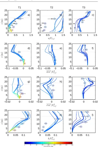
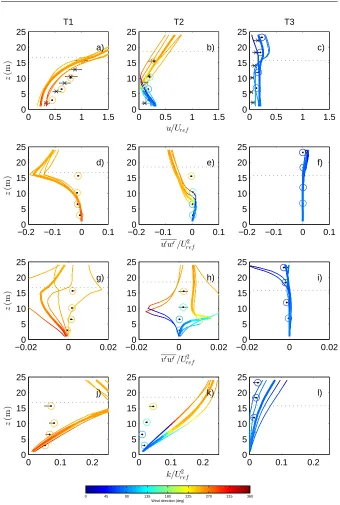
Figures 6 and 7 provide a more detailed comparison of the mean wind profiles
391
from the three towers, and also the profiles of momentum fluxes and turbulent
ki-392
netic energy. To allow for a more quantitative comparison between observations and
393
model the profiles are all normalised using a reference velocity Ure f which, for both
394
the observations and the model, is taken as the wind speed at the height of the
high-395
est instrument on the upwind tower (tower T1 for south-westerlies and tower T3 for
396
north-easterlies). This normalisation is to account for differences in the background
397
windspeed between the model and the different observations. Table 1 gives the value
0 0.5 1 1.5 0 5 10 15 20 25 a) z (m ) T1
−0.1 −0.050 0 0.05
5 10 15 20 25 d) z (m )
−0.020 0 0.02
5 10 15 20 25 g) z (m )
0 0.05 0.1
0 5 10 15 20 25 j) z (m )
0 0.5 1 1.5
0 5 10 15 20 25 b) u/Uref T2
−0.1 −0.050 0 0.05
5 10 15 20 25 e)
u′w′/U2
ref
−0.020 0 0.02
5 10 15 20 25 h)
v′w′/U2
ref
0 0.05 0.1
0 5 10 15 20 25 k) k/U2 ref
0 0.5 1 1.5
0 5 10 15 20 25 c) T3
−0.1 −0.050 0 0.05
5 10 15 20 25 f)
−0.020 0 0.02
5 10 15 20 25 i)
0 0.05 0.1
0 5 10 15 20 25 l)
Wind direction (deg)
0 45 90 135 180 225 270 315 360
Fig. 6 Profiles for the north-easterly case of (a-c) wind speed, (d-f) streamwise momentum flux u′w′,
(g-i) across-stream momentum flux v′w′and (j-l) turbulent kinetic energy, all normalised with a reference
velocity Ure ftaken at the height of the top instrument on the upstream tower T3. Symbols show the mean
value from the observations and the error bar shows the interquartile range. The coloured circles represent
measurements from the sonic anemometers, with the colour denoting the wind direction. The crosses are
measurements from the cup anemometers on the towers. The solid lines show interpolated model profiles at
the site of the tower (thick line) and at points 25m to the north, south, east and west of the tower (thin lines),
again coloured according to wind direction. The horizontal dotted line marks the approximate canopy top
[image:24.595.72.413.75.586.2]0 0.5 1 1.5 0 5 10 15 20 25 a) z (m ) T1
−0.20 −0.1 0 0.1
5 10 15 20 25 d) z (m )
−0.020 0 0.02
5 10 15 20 25 g) z (m )
0 0.1 0.2
0 5 10 15 20 25 j) z (m )
0 0.5 1 1.5
0 5 10 15 20 25 b) u/Uref T2
−0.20 −0.1 0 0.1
5 10 15 20 25 e)
u′w′/U2
ref
−0.020 0 0.02
5 10 15 20 25 h)
v′w′/U2
ref
0 0.1 0.2
0 5 10 15 20 25 k) k/U2 ref
0 0.5 1 1.5
0 5 10 15 20 25 c) T3
−0.20 −0.1 0 0.1
5 10 15 20 25 f)
−0.020 0 0.02
5 10 15 20 25 i)
0 0.1 0.2
0 5 10 15 20 25 l)
Wind direction (deg)
[image:25.595.71.411.79.584.2]0 45 90 135 180 225 270 315 360
Table 1 Values of the reference wind speed Ure f from the observations (median and interquartile range)
and from the model for the north-easterly and south-westerly cases.
Wind Reference Median wind Interquartile Model wind
direction tower (m s−1) range (m s−1) (m s−1)
NE T3 4.3 2.8 – 5.9 5.4
SW T1 10.0 7.9 – 12.5 3.7
for Ure f from the model and the median and interquartile range from the observations
399
for each wind direction. Several interpolated model profiles are shown, one from the
400
location of each tower and 4 more from 25 m north, south, east and west of the tower
401
(25 m is half the grid resolution of the model) to give an idea of the spatial variability
402
in the model, and hence the possible uncertainty in the model-observation
compari-403
son. It is worth noting that the mean wind speeds measured by the cup anemometers
404
are lower than those measured by the sonic anemometers as a result of stalling at low
405
wind speeds in the canopy. This problem is particularly noticeable in Fig 6(a)-(c) due
406
to the lower wind speeds in the north-easterly flow conditions.
407
For north-easterly cases (Fig 6) the model mean wind profiles at towers T1 and
408
T3 are in reasonable agreement with the observations, however the modelled
pro-409
files at tower T2 appear to significantly overpredict the wind speed, although they do
410
capture a profile with fairly constant wind speeds in the canopy and increasing wind
411
speeds above. There is also a large spread between the different model profiles
sug-412
gesting a region of complex canopy cover with large differences in wind speed over
413
short spatial distances. Bearing this is mind, along with the relatively simple
treat-414
ment of the canopy properties (uniform canopy height and density everywhere within
the canopy) it is perhaps not surprising that the model and observations show some
416
discrepancy. Tower T2 is characterised by quite different canopy cover to the east
417
(relatively sparse larch) and to the west (dense spruce), and there is a fire break to the
418
south, so the uniform canopy parameters are not necessarily a good approximation
419
at this location. Interestingly the profiles of streamwise momentum flux, u′w′, are in
420
good agreement at all three towers. Note also that there is very little variability in the
421
normalised observations of streamwise momentum flux, suggesting that the single
422
reference velocity at the top of tower T3 provides a good scaling for the momentum
423
flux. The relative accuracy of the streamwise momentum flux predictions at T2 is
424
likely to be due to the fact the model captures the right wind shear profile
through-425
out most of the canopy, it’s just that the wind speeds are consistently too large. In
426
contrast the profiles of v′w′show generally less good agreement between model and
427
observations. The model profiles do demonstrate a significant degree of variability
428
suggesting that v′w′is sensitive to the details of the local canopy and flow structure.
429
Comparisons of turbulent kinetic energy profiles between the model and observations
430
are also reasonable at T1 and T3, although at T2 the model appears to consistently
431
overpredict the turbulent kinetic energy within the canopy, which may be related to
432
the overprediction of the wind speeds in this case.
433
For south-westerly cases (Fig 7) the model mean wind profiles at T2 and T3 show
434
reasonable agreement with the observations, although the model seems to predict
435
more wind shear at T2 than is seen in the observations. At T1, the comparison is a
436
little less good, with the model underpredicting wind speeds below canopy top and
437
too strong a shear near canopy top. T1 is sat on a small outcrop, and in south-westerly
winds the flow is likely to accelerate over this outcrop, rather than passing through the
439
upwind canopy, but this feature is not well resolved by the model with the given 50m
440
horizontal resolution. Streamwise momentum fluxes are also in reasonable agreement
441
at most locations, except at the top of towers T1 and T2 where the model predicts a
442
much more rapid increase in the momentum flux than was observed. There is slightly
443
more wind shear in the model wind profiles, but not enough to account for the large
444
increase in momentum flux. The model profiles are very consistent and so this does
445
not appear to be due to spatial heterogeneity. It may be due to slight differences in
446
the canopy height between the model and observations, since the model assumes a
447
constant height of 15 m, or due to vertical variations in the canopy structure which are
448
not represented in the model simulation. Once again across-stream momentum fluxes
449
v′w′ are very variable and show little agreement between model and observations
450
except at T3. This highlights the very three-dimensional nature of the flow at T1
451
and T2. For the south westerly cases turbulent kinetic energy profiles seem to be
452
overpredicted by the model at most heights, even where the momentum fluxes are in
453
reasonable agreement. This is most pronounced at T1 and T2. The overprediction of
454
shear near the canopy top may lead to extra generation of turbulent kinetic energy in
455
the model, which is then mixed down into the canopy. A further possibility is that
456
the simple representation of dissipation used in the model is not correct in complex
457
heterogeneous canopies. Further work is needed to understand these discrepancies.
458
Overall the model reproduces surprisingly well the observed patterns of wind
459
speed and direction over the hill. Those sites where the agreement is less good appear
460
to be primarily located close to the forest edge or near the ridge top at tower T2.
The model also appears to often capture the observed streamwise momentum fluxes,
462
although the across-stream momentum fluxes and turbulent kinetic energy profiles
463
are not always captured as accurately. The agreement gives confidence in using the
464
model results to study more closely the patterns of mean flow and flow separation
465
over the ridge.
466
5 Flow separation and sensitivity to surface parametrization 467
The results of Ross and Vosper (2005) suggested that flow separation is an intrinsic
468
feature of uniform canopy flows over idealised hills, and that this is fundamentally
469
different to flow separation over a hill with a rough surface. Here the sensitivity of the
470
model results to the surface parametrization over a more complex and realistic hill is
471
investigated, with particular focus on flow separation.
472
To test the importance of explicitly resolving the canopy in these simulations the
473
westerly wind case was re-run with the forest canopy being represented by a
rough-474
ness length parametrization rather than with the explicit canopy model. The
rough-475
ness length was chosen to match the equivalent roughness of the canopy, z0=0.35
476
(see e.g. Ross and Vosper, 2005). All other aspects of the simulation were unchanged.
[image:29.595.50.414.245.651.2]477
Figure 8 shows the wind roses from this simulation. In comparison with Fig. 5 there
478
is clearly less strong flow separation with the roughness length parametrization of the
479
surface. The sites that would be in the canopy over the lee slope show a flow which
480
is slowed and deflected along the slope to the south rather than being completely
re-481
versed as occurs with the canopy model. Outside the canopy there is little difference
482
between the results, suggesting that the impact of the canopy is relatively localised. In
x(m)
y
(m
)
a)
ARA ARB
ARC ARE
ARF ARG
ARH ARJ
ARL ARN
ARP ARQ
0 400 800 1200 1600 2000
0 400 800 1200 1600 2000
T1 T2 T3
0 5 10 15 20 25
z
(m
)
b)
wind speed (m s
−1
)
[image:30.595.75.410.76.227.2]0 1 2 3 4 5 6 10 15
Fig. 8 Wind roses from the model simulation with westerly winds and a roughness length parametrization
of the canopy. Results are shown at the 12 AWS sites (a) and the 3 towers (b).
the vertical (not shown) the region in which the flow is reversed or strongly deflected
484
appears to extend up to about 55m above ground level (40m above the canopy top)
485
with the explicit canopy model. In contrast, with the roughness length
parametriza-486
tion the depth and horizontal extent of the region of strongly deflected flow is much
487
reduced, reaching a maximum height of only about 12m above ground level. This
488
suggests that even above the canopy, perhaps up to a couple of times the canopy
489
height, the flow may be fundamentally different under conditions of flow separation
490
depending on the way the effect of the canopy is modelled.
491
In three dimensions it is hard to identify flow separation in the velocity field.
Un-492
like in two dimensions it is not simply a matter of looking for reversed flow since the
493
flow may be deflected rather than reversed. This makes interpreting the flow pattern
494
based on point observations tricky. Using the model allows a better understanding of
495
the flow across the whole ridge, but it is still difficult to identify flow separation from
496
near surface winds. As Hunt et al. (1978) showed, flow separation is associated with
497
a singularity in the surface stress field and this can provide an alternative method for
identifying points or lines where the flow separates from or reattaches to the surface
499
in three-dimensional flows. The surface stress is given by∂us/∂n where usis the
ve-500
locity tangential to the surface and n is the normal to the surface and so the surface
501
stress gives an indication of the flow direction at the surface, but has the advantage
502
of being non-zero, except where flow separates or reattaches. Wood (1995) suggested
503
using plots of surface stress “streamlines” or streaks to identify these singularities.
504
The streaks are plotted by calculating a series of two-dimensional surface trajectories
505
(x,y), where the two horizontal components of the surface stress take the role of the
506
velocity field so
507
dx dt =τx
dy
dt =τy. (2)
The streaks are initialised from a series of points across the model domain and then
508
calculated by integrating the trajectories forward and backwards for a specified length
509
time. This works well for the examples used by Wood (1995), however the large
510
difference between surface stress values inside and outside the canopy means that
511
streaks in the canopy are very short. To circumvent this problem, we use a longer
512
integration time, but limit the length of the streaks plotted so that streaks outside
513
the canopy are not too long. The surface stresses are interpolated from the model
514
grid using bilinear interpolation and the integration is carried out using the ode45
515
function in Matlab. Using this approach and integrating forward numerically from
516
t=0 to t=20000, and limiting the length of the streaks to 500 m gives much more
517
even lengths of streaks inside and outside the canopy, and makes visualisation of flow
518
separation much easier in partially forested flows. Locations where the surface stress
519
streaks all converge at a line or point are associated with flow separating from the
surface, while locations where the surface stress streaks all diverge from a line or
521
point are associated with flow reattaching to the surface.
522
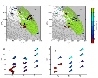
Figure 9 shows plots of the surface stress streaks calculated from the model.
For-523
ward trajectories (blue) show flow separation and backward trajectories (red) show
524
reattachment. Wind direction vectors are also plotted at the points where trajectories
525
are initiated. For the easterly wind simulation (Fig. 9a) the surface stress plot clearly
526
illustrates the flow separation occurring over the lee slope on the forested part of the
527
ridge. There is one clear separation line just upwind of the ridge summit stretching
528
right along the forested part of the ridge there is also some indication of a second
529
separation line downwind of the ridge on the southern shoulder of the ridge.
Reat-530
tachment appears to occur at a singular point on the lee slope close to x=1300 m
531
and y=1100 m. This highlights the rather complicated three-dimensional structure
532
of the flow separation over a real ridge with heterogeneous canopy cover in
compar-533
ison with previous idealised two-dimensional modelling and laboratory studies. To
534
the north where there is no forest cover then the stress streaks pass right over the
535
ridge showing that flow separation does not occur, even though the ridge is slightly
536
higher at this point. Around the southern edge of the ridge, outside the canopy the
537
stress streaks run more or less parallel to the lower edge of the canopy and the
con-538
tours. This demonstrates the importance of flow around the southern end of the ridge
539
in easterly flow.
540
In contrast, for the westerly case (Fig. 9b) where the steep eastern slope of the
541
ridge is on the downwind side there is clear evidence of flow separation all along
542
the summit of the ridge, with reattachment occurring somewhere off the coast. Even
without the forest canopy this slope is steep enough to generate flow separation. In
544
this case there is a single separation line running right down the ridge. Outside the
545
canopy the separation line is downwind of the ridge summit, while within the canopy
546
separation occurs nearer the ridge summit. The flow off the coast remains almost
547
parallel to the ridge and to the coastline, suggesting that the region of separated flow
548
extends well beyond the foot of the ridge and is therefore much larger than in the
549
easterly wind case. The streaks in this case also suggest a rather less important role
550
for flow around the southern end of the ridge in westerly flow. These figures support
551
the interpretation of the flow separation based on the observed and model wind fields
552
made above and highlight the differences between cases with steep lee slopes where
553
flow separation would occur anyway (westerly flow) and less steep lee slopes, where
554
flow separation requires the presence of the canopy (easterly flow).
555
The conclusions on the sensitivity of the results to the explicit canopy
parametriza-556
tion are supported by the surface stress plot for the roughness length simulations. For
557
the easterly wind case (Fig. 9c) no flow separation was observed at all in the
sur-558
face stress streaks with a roughness length parametrization, in clear contrast to the
559
simulation with an explicit canopy. For the westerly case (Fig. 9d) a clear
separa-560
tion line downwind of the summit of the ridge is apparent with the roughness length
561
parametrization. Outside the canopy the streaks look very similar in the two
sim-562
ulations. Inside the canopy, parametrizing the canopy by a roughness length shifts
563
the flow separation further down the lee slope, and significantly reduces the
variabil-564
ity caused by the heterogeneous canopy cover and channelling through gaps in the
565
canopy. Explicitly modelling the canopy appears to be essential to capture the flow
x(m)
y
(m
)
a)
0 400 800 1200 1600 2000
0 400 800 1200 1600 2000
x(m)
y
(m
)
b)
0 400 800 1200 1600 2000
0 400 800 1200 1600 2000
x(m)
y
(m
)
c)
0 400 800 1200 1600 2000
0 400 800 1200 1600 2000
x(m)
y
(m
)
d)
0 400 800 1200 1600 2000
[image:34.595.76.405.78.409.2]0 400 800 1200 1600 2000
Fig. 9 Surface stress streaks from the model (forward trajectories - blue lines, backward trajectories - red
lines) plotted over the height contours (at 10m intervals). Also plotted are wind direction arrows. Results
are shown for easterly (a, c) and westerly (b, d) winds. Subfigures a), b) are with the explicit canopy model
and c), d) are with a roughness length parametrization of the canopy. The orange dots show the sites of the
AWS.
separation in the easterly case with a shallow lee slope, and even in the westerly case
567
with a steeper lee slope the explicit canopy model significantly changes the location
568
and magnitude of the separated region.
6 Discussion and conclusions 570
Flow over realistic complex terrain with variable forest cover, such as the Leac Gharbh
571
ridge, is complicated and the local wind direction depends strongly on the local
ter-572
rain and forest cover. Burns et al. (2011), one of the few other observational studies in
573
complex terrain, draws similar conclusions. For flow which is close to neutral, high
574
resolution numerical simulations with an explicit canopy model reproduce many of
575
the features of the observed flow, however high quality input data sets for the terrain
576
and the forest canopy are essential. High resolution terrain data sets are generally
577
available, however details of forest canopy parameters are generally harder to obtain
578
and require dedicated surveys. Available mapping products may provide details of
579
the forest coverage, but they rarely contain details on the nature of the forest, the
580
canopy height, or the canopy density. These details are essential for successful
mod-581
elling of the flow in or near the canopy. Other recent studies (Burns et al., 2011;
582
Desmond et al., 2014; Schlegel et al., 2015) have also highlighted the need for
de-583
tailed canopy structure to accurately model heterogeneous canopy flows. Indeed in
584
their study Desmond et al. (2014) saw more sensitivity to realistic canopy structure
585
(particularly vertical structure) than they did to the turbulence closure model used.
586
Recent progress using lidar offers exciting possibilities for detailed three-dimensional
587
mapping of canopy structure (Boudreault et al., 2015), but unfortunately such a
sur-588
vey was not available at this site.
589
Near the edge of the forest canopy there appears to be greater discrepancy
be-590
tween the model and observations. This is partly due to the limitations of the forestry
591
data, but more fundamentally may be linked to the horizontal resolution of the