Solar radiation and functional traits explain the decline of forest primary productivity along a tropical elevation gradient

This is a repository copy of Solar radiation and functional traits explain the decline of forest primary productivity along a tropical elevation gradient.

White Rose Research Online URL for this paper: http://eprints.whiterose.ac.uk/118230/

Version: Supplemental Material

Article:

Fyllas, NM, Bentley, LP, Shenkin, A et al. (17 more authors) (2017) Solar radiation and functional traits explain the decline of forest primary productivity along a tropical elevation gradient. Ecology Letters, 20 (6). pp. 730-740. ISSN 1461-023X

https://doi.org/10.1111/ele.12771

© 2017 John Wiley & Sons Ltd/CNRS. This is the peer reviewed version of the following article: Fyllas, NM, Bentley, LP, Shenkin, A et al. (17 more authors) (2017) Solar radiation and functional traits explain the decline of forest primary productivity along a tropical elevation gradient. Ecology Letters, 20 (6). pp. 730-740., which has been published in final form at https://doi.org/10.1111/ele.12771. This article may be used for non-commercial purposes in accordance with Wiley Terms and Conditions for Self-Archiving.

[email protected] https://eprints.whiterose.ac.uk/ Reuse

Items deposited in White Rose Research Online are protected by copyright, with all rights reserved unless indicated otherwise. They may be downloaded and/or printed for private study, or other acts as permitted by national copyright laws. The publisher or other rights holders may allow further reproduction and re-use of the full text version. This is indicated by the licence information on the White Rose Research Online record for the item.

Takedown

If you consider content in White Rose Research Online to be in breach of UK law, please notify us by

1

Supporting Information

S1. Study Sites and Stand Productivity Estimation

Our study area is located along a 3300 m elevation gradient in the tropical Andes and extends to the

Amazon Basin. Across this transect a group of ten intensively monitored 1-ha plots was established

as part of the long-term research effort coordinated by the Andes Biodiversity Ecosystems Research

Group (ABERG, http://www.andesconservation.org) and the ForestPlots (https://www.forestplots.net/) and Global Ecosystems Monitoring Network (GEM;

http://gem.tropicalforests.ox.ac.uk/projects/aberg) networks. In this study we exclude SPD-02, which is located on a landslide prone ridge just below cloud and was always an outlier in our

simulations as well as in other studies across the gradient (Malhi et al. 2017a). Table S1.1 provides

a summary of the environmental conditions for the study sites. Five of the plots are montane plots

in the Kosñipata Valley, spanning an elevation range 1500 - 3500 m (Malhi et al. 2010), two are

submontane plots located in the Pantiacolla front range of the Andes (range 600 - 900 m) and two

plots are found in the Amazon lowlands in Tambopata National Park (elevation range 200 - 225 m).

The elevation gradient is very moist (Table S1.1), with seasonal cloud immersion common above

1500 m elevation (Halladay et al. 2012), and no clear evidence of seasonal or other soil moisture

constraints throughout the transect (Zimmermann et al. 2010). Plots were established between 2003

and 2013 in areas that have relatively homogeneous soil substrates and stand structure, as well as

minimal evidence of human disturbance (Girardin et al. 2014).

At all plots, the GEM protocol for carbon cycle measurements was employed

(www.gem.tropicalforests.ox.ac.uk). The GEM protocol involves measuring and summing all major components of NPP and autotrophic respiration on monthly or seasonal timescales (Malhi et al.

2017a). NPP measurements include: canopy litterfall, leaf loss to herbivory, aboveground woody

productivity of all medium-large (D>10 cm) trees (every three months), annual census of wood

productivity of small trees (D 2-10 cm), branch turnover on live trees, fine root productivity from

ingrowth cores installed and harvested (every three months) and estimation of coarse root

productivity from aboveground productivity. Autotrophic respiration (Ra) is calculated by summing

up rhizosphere respiration (measured monthly), aboveground woody respiration estimated from

stem respiration measurements (monthly) and scaling with surface area, belowground coarse root

and bole respiration (fixed multiplier to stem respiration) and leaf dark respiration estimated from

measurements of multiple leaves in two seasons. GPP, the carbon assimilated via photosynthesis is

approximately equal to the amount of carbon used for NPP and Ra, thus GPP=NPP + Ra. Finally the

2

For six of the plots, NPP and GPP were estimated by summation of the measured and estimated

components of NPP and autotrophic respiration (Malhi et al. 2017a). For the remaining plots, we

used measured NPP to estimate GPP applying the mean carbon use efficiency of the other plots,

separated into cloud forest and submontane/lowland plots.

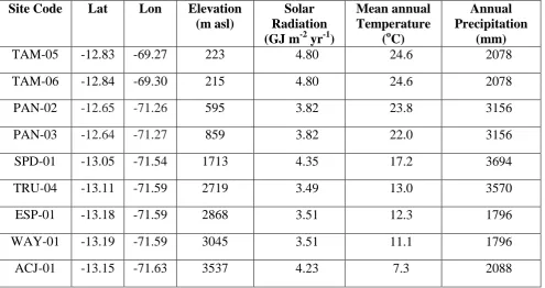
Table S1: Environmental characteristics of the study sites. Note that the annual solar radiation, mean temperature and total precipitation values refer only to year 2013.

Site Code Lat Lon Elevation (m asl)

Solar Radiation (GJ m-2 yr-1)

Mean annual Temperature

(oC)

Annual Precipitation

(mm)

TAM-05 -12.83 -69.27 223 4.80 24.6 2078

TAM-06 -12.84 -69.30 215 4.80 24.6 2078

PAN-02 -12.65 -71.26 595 3.82 23.8 3156

PAN-03 -12.64 -71.27 859 3.82 22.0 3156

SPD-01 -13.05 -71.54 1713 4.35 17.2 3694

TRU-04 -13.11 -71.59 2719 3.49 13.0 3570

ESP-01 -13.18 -71.59 2868 3.51 12.3 1796

WAY-01 -13.19 -71.59 3045 3.51 11.1 1796

ACJ-01 -13.15 -71.63 3537 4.23 7.3 2088

3

S2. Model Description

The original TFS model is a trait-continua and individual-based model, which simulates the carbon

(C) balance of each tree in a stand (Fyllas et al. 2014). The model is initialised with tree-by-tree

diameter at breast height (D) and functional traits data. Four functional traits [leaf dry mass per area

(LMA in g m-2), leaf N (NLm in mg g-1) and P (PLm in mg g-1) mass-based concentrations and wood

density W (g cm-3)] are used to represent a continuum of tree functional properties. Rather than

grouping trees into plant functional types, TFS implements distributions of functional traits and thus

a continuum of plant strategies and responses to environmental conditions can be simulated. Leaf

mass per area, wood density and maximum tree height seem to consistently influence competitive

interactions across plant species (Kunstler et al. 2016) and can be good candidate traits to represent

the global “fast-slow” plant economics spectrum (Reich 2014). In TFS, the three leaf traits (LMA, NLm, PLm), the central components of the leaf economic spectrum, regulate the photosynthetic

capacity and the respiration rate of trees (Wright et al. 2004, Atkin et al. 2015). Wood density ( W)

accounts for variation in aboveground biomass (MA in kg DM), with trees of greater W supporting

a higher biomass for a given D and tree height (Chave et al. 2014). Alllometric equations are used

to infer tree height (H in m) and allocation to leaf (ML), stem (MS) and root (MR) biomass (all in in

kg DM). Light competition is approximated through the perfect plasticity assumption, with tree H

used to estimate the relative position of an individual within the canopy, and thus the available solar

radiation (Strigul et al. 2008). The carbon and water balance of each tree is estimated on a daily

time-step and at the end of each simulation year, stand-level GPP and NPP is estimated by summing

up the daily individual-tree C fluxes.

The version of the model used in this study replaces the original CO2 assimilation [coupled

Farquhar - stomatal conductance model, Fyllas et al. (2014)] and C allocation algorithms with the

growth equation of Enquist et al. (2007b). Here we give a detailed description of the model,

emphasising on the coupling of the integrative growth equation with the climate and solar radiation

components of TFS. In particular the model of Enquist et al. (2007b) does not include any

temperature or light availability effects on leaf photosynthetic rates and thus spatial and temporal

variation of the thermal and irradiance conditions cannot be specifically modelled. We address these

shortcomings by allowing the model to estimate an individual-specific daily growth that is driven

by variation in temperature and irradiance (and potentially soil moisture) using the algorithms

4

1. Tree Allometry

The diameter at breast height (D in cm) along with the four functional traits of (LMA, NLm, PLm and

W) is used to functionally define each tree in a plot. For each study site the model is initialised with

measured tree D and trait values. Allometric equations relating tree height (H) and crown area (CA)

were taken from Shenkin et al. (2016, under review). In all cases mixed-effect linear regression

models were fit to account for species (fixed) and site (random) effects. The general form of these

equations is implemented in TFS. Tree height (in m) is estimated from D (cm):

10

exp(

log ( )) (1)

H









D

with H = 1.51 and H = 0.084

The exponent of the CA versus D scaling relationship is considered well conserved across tropical

tree species (Farrior et al., 2016), and this was also verified from the analysis of our data. Crown

area (in m2) is given from:

D (2)

A C

C





with C = 0.695 and C = 1.305

Aboveground tree biomass (MA in kg) is estimated from Chave et al. (2014) equation:

A

2

A A

(

)

(3)

M











D H

with A = 0.0673 and A = 0.976 and thus for a given D, trees with greater W achieve a greater MA.

Leaf (ML), stem (MS) and root (MR) biomass (all in kg) are calculated from aboveground biomass:

L

S

R

L L A

S S A

R R A

(4a)

(4b)

(4c)

M

M

M

M

M

M













The coefficients of these equations were estimated by fitting standardised major axis (SMA) lines

with data from the BAAD dataset (Falster et al. 2015). We only used data from evergreen

angiosperms species found in tropical rainforests and tropical seasonal forests with D>1cm, as

within our plots most species are evergreen and only individuals of D>2 cm are included in the

productivity calculations. In our simulations, in order to account for potential variation across

individual tree architecture we allowed the allometric coefficients to vary within the 95%

confidence intervals estimated by the SMAs (Fig S2.1). Total tree biomass is then given from:

(5)

T L S R

5

We note that for the simulations performed in this study the estimation of MS, MR and MT are not

required, as the growth rate of trees is expressed only as a function of foliage mass (equation 6).

Equation 3 adequately predicted MA when compared with the records reported in BAAD (Fig S2.1).

The range of ML allometries allowed within our simulations is illustrated in Fig S2.1.

Figure S2.1: Allometric equations used to predict total aboveground biomass (MA) and total dry leaf biomass (ML). Left panel: Red squares indicate predictions from the Chave et al. (2014) equation (equation 3) and black circles measurements reported in the BAAD dataset (Falster et al. 2016). The RMSE for predicted and reported MA was 143 kg. Right panel: The allometric relationship between dry leaf biomass (ML) and MA. The black line represents the power function

L

L L A

M  M with L=0.158 and L=0.707, while the broken lines indicate the range of allometries allowed in our simulations within the 95% CI of the SMA estimates [ L=(0.150 – 0.166) and

L=(0.690 – 0.724)].

2. Tree Growth

The relative growth rate (RGR) of a plant (the rate of increase in plant mass per unit of mass

present) can be factored to the following three components: the leaf net carbon assimilation rate, the

leaf area per unit leaf mass and the leaf weight ratio (Hunt 1982; Lambers et al. 2008). Enquist et al.

(2007b) extended this equation to include additional functional traits and the effect of plant size on

growth rate:

,

(

)(

)

(6)

T L

L D L

L

dM

c

a

A

M

dt





m

where M is the total plant dry biomass (kg), c the carbon use efficiency (no units), the fraction of

6

aL the individual leaf area (cm2), mL the individual leaf mass (g) and ML the total leaf dry mass (kg). The time step in our simulations (dt) is daily.

In our simulations a random carbon use efficiency (c) is assigned to each tree in a plot, drawing

from a normal distribution c( , )c  with c 0.33 and =0.04, the values estimated from field

observations at the plot level, which found no trend in c with elevation (Malhi et al. 2017a). The

term is set constant to 0.5 (gC g-1DM). The expression of the photosynthetic rate AL,D is also

extended here to account for inter- and intra- specific variability due to leaf traits as well as to light

availability (see Photosynthesis section). The L/mL ratio is the inverse of LMA (i.e. SLA) and it is

allowed to vary across individual trees.

The basic assumption in equation 6 is that whole-plant net biomass growth rate scales isometrically with total plant leaf biomass (Hunt 1982). However, predicting the patterns of plant biomass allocation is a topic of extensive debate with Metabolic Scaling Theory (MST) suggesting relative invariant power laws (Enquist et al. 2007a) and other studies showing that scalling varies across species and plant sizes (Poorter et al. 2015). Another critique of MST-based growth equations is that they do not take into account resources availability, for example light in forest stands (Muller-Landau et al. 2006, Coomes & Allen 2009). In order to implement equation 6 within TFS and deal with the above critics we 1) used a set of allometric equations with stochastic scaling coefficients estimated from available data and 2) expressed the photosynthetic rate AL,D as a

function of both leaf traits (that vary in a continuous way across individual trees) and irradiance that takes into account competition for light between individuals.

As discussed in the previous section (Tree Allometry) the scalling coefficient, L, of the L

L L A

M  M relationship is allowed to vary across our simulations within the (0.690 – 0.724) range predicted from the SMA fits of the BAAD dataset. This coefficient is usually denoted as in

MST studies (Enquist et al. 2007a) and can be considered as an additional “functional trait” that

reflects the geometry of the branching network. The exact value of has been vigorously debated

with recent analyses suggesting that it ranges in a continuous way with ontogeny and decreases

from seedlings to mature trees (Poorter et al. 2015). We note however that in our simulations the

smallest tree included had an MA≈3x103 g DM and the biggest one an MA≈23x106 g DM suggesting

that within this range the L scalling exponent could vary from ca 0.7 to 0.58 (Poorter et al. 2015),

being at a relative stable region. The sensitivity analysis of the model to variation in the L

parameter can be found in Fig S2.6. This analysis indicates that GPP and NPP simulations are

sensitive to the value of L value although this should change in combination with the normalization

7

3. Light Competition

One of the key criticisms of MST-based growth equations is that they fail to model asymmetric

competition for light (Muller-Landau et al. 2006, Coomes and Allen 2009). In order to account for

light competition between trees, we allowed AL,D to vary not only due to the functional properties of

a tree's foliage but also based on its relative position within the canopy. Light availability (I) for

each individual in the stand is estimated using the built-in canopy structure algorithm of TFS

(Fyllas et al. 2014), based on the Perfect Plasticity Approximation (PPA - Purves et al. 2008). In the

original TFS model, trees are classified at a canopy or sub-canopy group, with the latter group

receiving less radiation. Here we use a more detailed light availability profile, where more than one

canopy layers can be identified within a plot (Strigul et al. 2008). A critical height ( ) is estimated

for each layer (L). Trees that are taller than , i.e. canopy trees, receive the full amount of daily

radiation. Trees with height between and , are shaded by the first layer and so on. Each

layer is assumed to have a constant leaf area index equal to the ratio of the total stand‟s LAI with

the number of canopy layer identified. Based on its relative position within the canopy (number of

shading layers), light availability for each tree is estimate following the Beer‟s light extinction

model with an extinction coefficient K=0.5. Our simulations suggest that accounting for

asymmetric light competition is important in order to adequately simulate forest productivity along

the study gradient (S5 - Light Competition).

Bohlman and Pacala (2012) applied a similar multilayer version of the PPA model in Barro

Colorado Island and noted that the understorey layers (L>1) are probably not continuous and

coherent. Thus in our implementation of the PPA, where layers are considered continuous, their

relative importance for shading is probably overestimated in contrast with the underestimation of

the first (L=1) canopy layer. Both Bohlman and Pacala (2012) and Farrior et al. (2016) used PPA to

approximate light competition but implemented species independent growth rates within their

simulations. Our approach further enhances their approach, by also considering continuous

between-tree variation in potential growth rates emerging from differences in individual-tree

functional traits.

4. Photosynthesis

In order to account for inter- and intra- specific variability in the leaf specific photosynthetic rates

we used an independent dataset of 136 (one leaf per tree) light response curves and leaf traits

measurements in 14 plots along the Amazon-Andes gradient (Atkin et al. 2015; Weerasinghe 2015), and expressed AL,D (equation 6) as a function of the three (LMA, NLm and PLm ) functional traits. There

8

sites, although the elevation range covered (ca 100 to 3450 m asl), includes most of our study sites

with the exception of the uppermost plot (ACJ-01, 3537 m asl).

The light-response curve measurements were made using one cut branch per tree, with

measurements of net CO2 exchange (Anet) taking place between 10.00 am and 3.00 pm.

Measurements were made on the most recently fully expanded leaves attached to the cut branches

(which had been re-cut under water immediately after harvesting to preserve xylem water

continuity) using the LICOR 6400XT system (LI-COR Inc., Lincoln NE, USA). The block

temperature was set to that of the prevailing air temperature at each site at the time of measurements

(20°C at the upland sites, and 28°C at the lowland sites). The area-based net photosynthetic rate

(Anet µmol m-2 s-1) was measured starting at 2000 µmol photons m-2 s-1 and gradually decreased to darkness via 1500, 1000, 250, 100, 80, 60, 55, 50, 45, 40, 35, 30, 25, 20, 15, 10, 5 and 0 µmol

photon m-2 s-1 with relative humidity between 60-70% and CO2 concentration set at 400 ppm. An

equilibrium period of two minutes was allowed at each irradiance level before Anet was measured.

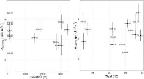
The plot-level analysis of this dataset (136 leaves/trees) suggest that the area-based net

light-saturated photosynthetic rate (at 1500 mol photons m-2 s-1) at the prevailing air temperature

(Anet1500) did not show any trend with elevation or leaf temperature (Fig S2.2). This is in agreement

with the findings of Malhi et al. (2017a), where at ambient temperatures there was no evidence of a

trend of photosynthetic parameters with elevation.

A recent study reported that, along the Andean elevation gradient, maximum carboxylation and

electron transport rates at a measurement temperature of 25oC were significantly higher at upland

sites, possibly reflecting greater P per unit leaf area at high elevations and/or thermal acclimation to

sustained lower growth temperatures (Bahar et al. 2016). By contrast, when measurements of gas

exchange were made at late morning to early afternoon at each site (20-28oC; Fig S2.2),

light-saturated, area-based rates of net photosynthesis, as well as maximum carboxylation and electron

transport rates, show no significant trend with elevation (Bahar et al. 2016, Malhi et al. 2017a). The

latter observations support the use of a temperature-independent equation for photosynthetic carbon

assimilation in our simulations. We note, however, that our photosynthetic light response curves

were parameterised with measurements made at leaf temperatures higher than 20oC. For some of

the upland sites, leaf temperatures are lower than 20oC for much of the day (van de Weg et al.

2014). This raises the question of whether our estimates of daytime carbon-fixation are an

overestimate, given the potential for lower temperatures to reduce net photosynthesis. Currently,

there are few data available on how leaf temperatures less than 20°C affect maximum

photosynthetic rates along tropical elevation gradients such as that in Peru. A recent study in

tropical montane forests in Rwanda showed that while the optimum temperature for photosynthesis

9

temperature range over which optimal rates are exhibited is broad, such that rates at 20°C and 25°C

are similar (Varhammar et al. 2015). If the same is true for species adapted to our Andean high

elevation plots, then maximum photosynthesis may be relatively temperature insensitive across the

dominant daily range of leaf temperatures experienced (i.e. our measurements of leaf

photosynthesis would be indicative of carbon uptake rates across a wider range of temperatures

experienced by leaves each day at high altitude). Thus although trees in higher elevations operate

under lower temperatures, their maximum light-saturated photosynthetic rate is equivalent to their

lowland counterparts. The fact that in our dataset Anet1500 is higher than would be expected at lower

temperatures (upland plots) is because of the higher photosynthetic capacity of the trees found at

higher elevations.

Figure S2.2 Plot average net light-saturated (at 1500 mol photons m-2 s-1) photosynthetic rate (±standard error) at prevailing air temperature against site elevation and average leaf temperature.

σo trend was observed in either case (Kendall‟s = -0.209, p = 0.331 and =0 .077, p = 0.747).

Measurements of the instantaneous net photosynthetic rate (Anet) at different light intensities

were subsequently used to fit the Michaelis-Menten (MM) light response model for each curve. The

MM model was fit by applying the Differential Evolution (DE) algorithm (DEoptim R-package) to minimise the sum of squares. Chen et al. (2016) have shown that the DE provides robust estimates

for various photosynthetic light response models and it is not sensitive to initial values selection.

The MM light response model is given by the following equation:

max

(7)

net d

A I

A R

k I

 

10

where I ( mol m-2s-1) the irradiance, Amax the maximum gross photosynthetic rate ( mol m-2 s-1), k

the half saturation coefficient ( mol m-2

s-1) and Rd is the non-photorespiratory mitochondrial CO2

release taking place in the light (i.e. respiration in the light) ( mol m-2 s-1). The low light part (I<60

mol m-2

s-1) of the curve was excluded in order to minimize the effects of the „Kok effect‟ (Kok

1948), as the inhibitory effect of light diminishes as irradiance approaches darkness, resulting in

increased rates of respiration in darkness compared to those in the light (e.g. Weerasinghe et al.

(2014)).

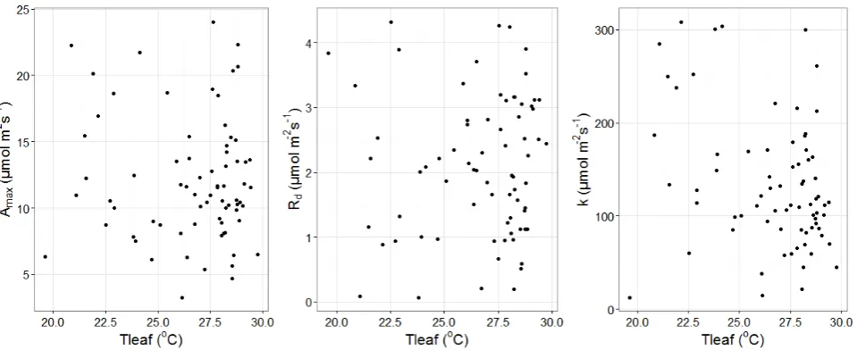
As for some curves the MM parameter estimates were unreasonable, we only used individual

curves with estimates of Rd>0 ( mol m-2 s-1), Rd<4.5 ( mol m-2 s-1) and k<400 ( mol m-2 s-1) for

further analysis (72 curves). Figure S2.3 illustrates the leaf-specific estimates of MM model for

each light response curve versus average leaf temperature. No trend of Amax nor Rd was found with

leaf temperature, in agreement with the constant Anet1500 at ambient temperatures. On the other hand,

the estimated half saturation coefficient (k) presented a decreasing trend with leaf temperature

(Kendall‟s = -0.19, p = 0.018).

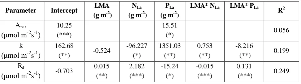
Figure S2.3: Leaf-specific estimates of the Michaelis Menten light response curve parameters versus leaf temperature. No trend was identified in Amax and Rd with leaf temperature, while k decreased with leaf temperature (Kendall‟s = -0.19, p = 0.018).

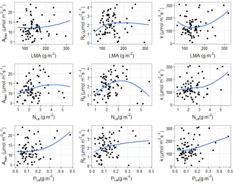
We initially explored how the estimated parameters of the MM equation (Amax, k, Rd) varied (Fig

S2.4) with the three leaf traits, expressed on an area basis (LMA, NLa and PLa). Amax increased with

PLa supporting the role of leaf P in controlling leaf photosynthesis in tropical forests, Rd increased

with LMA and PLa with higher P concentration associated with higher ATP and greater

physiological activity and respiration and k increased with NLa in accordance with protein rich

11

Figure S2.4: Variation of the Michaelis-Menten light response curve parameters against individual

leaf traits. The blue lines present local polynomial regressions.

We subsequently used a backward stepwise multiple linear regression to express Amax, Rd and k

as a function of the three leaf traits with the initial model including second level interactions of

LMA with the two leaf nutrient concentrations (NLa and PLa). The final models (Table S2.1) were

selected by the Akaike information criterion (AIC) criterion. Amax was only related to PLa with the

model explaining only the 5% of the variation, and thus the overall mean 12.13 ( mol m-2

s-1) was

considered as the common maximum photosynthetic rate for all trees. The half saturation

coefficient (k) was mainly related to leaf nutrients, with the linear model accounting for 20% of

variation in k (Table S2.1). Finally, Rd was related to all three leaf traits with the linear model

accounting for ca 25% of the variation. These equations were used to parameterise the TFS light

response model that accounts for the effects of trait variation on the photosynthetic properties of

individual leaves.

An average daily photosynthetic rate AL (gC m-2 day-1) is estimated for each tree with the

12

average daily light availability is used in equation (7), which is converted to photosynthetic photon

flux density (PPFD) assuming a 0.48 PAR to solar short-wave radiation ratio and a solar PAR to

conversion factor of 4.6 mol J-1. Total foliage absorptance was assumed to be 0.75 (Valladares et

al. 2002). The total daily photosynthetic rate AL,D (equation 6) is estimated by multiplying average

AL with the day length.

Table S2.1: Summary of the multiple linear regression models for the parameters of the Michaelis-Menten light response function (dependent variables) and the leaf functional traits (predictors).

Parameter Intercept LMA

(g m-2)

NLa (g m-2)

PLa (g m-2)

LMA* NLa LMA* PLa

R2

Amax

( mol m-2 s-1)

10.25 (***)

15.51

(*) 0.056

k ( mol m-2

s-1)

162.68

(**) -0.524

-96.227 (*) 1351.03 (**) 0.753 (**) -8.216

(**) 0.199

Rd

( mol m-2

s-1) -0.703

0.015 (**) 2.182 (***) -15.24 (*) -0.015 (***) 0.131

(***) 0.249

5. Temperature Sensitivity

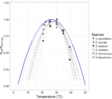
Although the analysis of the photosynthetic rates data along the elevation gradient support the use

of a temperature independent photosynthetic model, we specifically explored whether including a

photosynthetic temperature dependence could increase the predictive ability of TFS. For that

purpose we employed a normalised temperature response function (Higgins et al. 2016):

2

g(T)=max(0,-0.242+0.0937T-0.00177T ) (8)

ranging between 0 and 1 and used as a multiplier for Anet. The shape of equation 8 was validated

against photosynthetic temperature responses data from montane rainforest species in Rwanda

(Varhammar et al 2015). Anet data of six species at different temperatures were provided

(Varhammar pers. comm) and the ratio of Anet to the maximum Anet measured across the

temperature range was estimated. Quadratic curves were fitted for each species and each curve was

plotted against the generic model (Fig S2.5). The temperature sensitivity function is used to account

for the effects temperature variation on daily photosynthesis. We note that the generic temperature

sensitivity model yield a wider curve and thus leads to smaller reductions of Anet for given

temperature changes compared with the available data. We note that this is the only temperature

dependence of the model, as one of our questions was to explore whether explicitly taking into

13

Fig S2.5. Temperature sensitivity function (blue curve) used in our simulations following the

generic model of Higgins et al. (2016). Available data from montane species (broken lines) in

Rwanda are also plotted. The thicker broken line represents the average temperature sensitivity

across all species.

6. Stand level primary productivity.

The above equations are applied for each individual within the stand to estimate a daily and at the

end of each year an annual growth, i.e. the tree specific NPP. The GPP of each tree is estimated by

dividing with the individual specific carbon use efficiency c. The stand level GPP and NPP are

estimated by summation of all individual NPPs and GPPs.

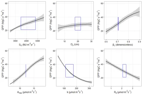
7. Sensitivity Analysis

We performed a sensitivity analysis of the simulated GPP by systematically changing the values of

a set of key parameters, including the total solar radiation at the top of the canopy So, the mean

diameter of the trees (with no change in total stand Basal Area), the value of the L (or ) scalling

exponent, as well as the values of the maximum gross photosynthesis (Amax), the half saturation

14

the outputs from the sensitivity analysis. A similar sensitivity of simulated NPP was observed and

results are not reported here.

Fig S2.6. Sensitivity analysis of simulated GPP to changes in some key model parameters. The

black lines indicate local polynomial regressions of the mean GPP across all plots and the grey area

the 95% confidence interval. The area within the blue rectangular shape indicates the range of GPP

and the respective model parameter within our simulations.

Simulated GPP was sensitive to changes of radiation So at the top of the canopy with a doubling

of So leading to a doublinf of GPP. Sensitivity to average stand diameter (D ) was explored by

maintaining the total stand basal area (BA) and changing the relative size of individual trees.

Overall the model was not very sensitive to changes of D suggesting that the relative contribution

of different size classes in the total biomass of the stand is not a strong driver of productivity in the

model. Simulated GPP was also sensitive to variation of the scaling exponent of the allometric

relationship L

L L A

M  M , with higher L leading to simulations of higher productivity. We note

that in the sensitivity analysis we systematically changed L without changing L. However L

should co-vary with L and thus these simulations are oversensitive to changes in L. The model

was also sensitive to variation of the parameters of the photosynthetic light response curve, with

15

References

1.Atkin, O.K., Bloomfield, K.J., Reich, P.B., Tjoelker, M.G., Asner, G.P., Bonal, D., et al. (2015). Global variability in leaf respiration in relation to climate, plant functional types and leaf traits. New Phytol, 206, 614–636

2.Bahar, σ.H.A., Ishida, F.Y., Weerasinghe, L.K., Guerrieri, R., τ‟Sullivan, τ.S., Bloomfield, K.J.,

et al. (2016). Leaf-level photosynthetic capacity in lowland Amazonian and high-elevation Andean tropical moist forests of Peru. New Phytol, n/a-n/a

3.Bohlman, S. & Pacala, S. (2012). A forest structure model that determines crown layers and partitions growth and mortality rates for landscape-scale applications of tropical forests. Journal of Ecology, 100, 508–518

4.Chave, J., Réjou-Méchain, M., Búrquez, A., Chidumayo, E., Colgan, M.S., Delitti, W.B., et al. (2014). Improved allometric models to estimate the aboveground biomass of tropical trees. Global change biology, 20, 3177–3190

5.Chen, L., Li, Z.-B., Hui, C., Cheng, X., Li, B.-L. & Shi, P.-J. (2016). A general method for parameter estimation in light-response models. Scientific Reports, 6, 27905

6.Coomes, D.A. & Allen, R.B. (2009). Testing the Metabolic Scaling Theory of tree growth. Journal of Ecology, 97, 1369–1373

7.Enquist, B.J., Allen, A.P., Brown, J.H., Gillooly, J.F., Kerkhoff, A.J., Niklas, K.J., et al. (2007a). Biological scaling: Does the exception prove the rule? Nature, 445, E9–E10

8.Enquist, B.J., Kerkhoff, A.J., Stark, S.C., Swenson, N.G., McCarthy, M.C. & Price, C.A. (2007b). A general integrative model for scaling plant growth, carbon flux, and functional trait spectra. Nature, 449, 218–222

9.Falster, D.S., Duursma, R.A., Ishihara, M.I., Barneche, D.R., FitzJohn, R.G., Vårhammar, A., et al. (2015). BAAD: a Biomass And Allometry Database for woody plants. Ecology, 96, 1445– 1445

10.Farrior, C.E., Bohlman, S.A., Hubbell, S. & Pacala, S.W. (2016). Dominance of the suppressed: Power-law size structure in tropical forests. Science, 351, 155–157

11.Fyllas, N.M., Gloor, E., Mercado, L.M., Sitch, S., Quesada, C.A., Domingues, T.F., et al. (2014). Analysing Amazonian forest productivity using a new individual and trait-based model (TFS v.1). Geosci. Model Dev., 7, 1251–1269

12.Girardin, C.A.J., Espejob, J.E.S., Doughty, C.E., Huasco, W.H., Metcalfe, D.B., Durand-Baca, L., et al. (2014). Productivity and carbon allocation in a tropical montane cloud forest in the Peruvian Andes. Plant Ecology & Diversity, 7, 107–123

13.Halladay, K., Malhi, Y. & New, M. (2012). Cloud frequency climatology at the Andes/Amazon transition: 1. Seasonal and diurnal cycles. J. Geophys. Res., 117, D23102

14.Higgins, S.I., Buitenwerf, R. & Moncrieff, G.R. (2016). Defining functional biomes and monitoring their change globally. Glob Change Biol, 22, 3583–3593

15.Hunt, R. (1982). Plant growth curves. The functional approach to plant growth analysis. Plant growth curves. The functional approach to plant growth analysis.

16.Kok, B. (1948). A critical consideration of the quantum yield of Chlorella-photosynthesis. W. Junk

16

18.Lambers, H., Chapin, F.S. & Pons, T.L. (2008). Plant Physiological Ecology. Springer New York, New York, NY

19.Malhi, Y., Girardin, C.A.J., Goldsmith, G.R., Doughty, C.E., Salinas, N., Metcalfe, D.B., et al. (2016). The variation of productivity and its allocation along a tropical elevation gradient: a whole carbon budget perspective. New Phytol, n/a-n/a

20.Malhi, Y., Silman, M., Salinas, N., Bush, M., Meir, P. & Saatchi, S. (2010). Introduction: Elevation gradients in the tropics: laboratories for ecosystem ecology and global change research. Global Change Biology, 16, 3171–3175

21.Muller-Landau, H.C., Condit, R.S., Chave, J., Thomas, S.C., Bohlman, S.A., Bunyavejchewin, S., et al. (2006). Testing metabolic ecology theory for allometric scaling of tree size, growth and mortality in tropical forests. Ecology Letters, 9, 575–588

22.Poorter, H., Jagodzinski, A.M., Ruiz-Peinado, R., Kuyah, S., Luo, Y., Oleksyn, J., et al. (2015). How does biomass distribution change with size and differ among species? An analysis for 1200 plant species from five continents. New Phytol., 208, 736–749

23.Purves, D.W., Lichstein, J.W., Strigul, N. & Pacala, S.W. (2008). Predicting and understanding forest dynamics using a simple tractable model. PNAS, 105, 17018–17022

24.Reich, P.B. (2014). The world-wide “fast–slow” plant economics spectrum: a traits manifesto. J Ecol, 102, 275–301

25.Strigul, N., Pristinski, D., Purves, D., Dushoff, J. & Pacala, S. (2008). Scaling from trees to forests: tractable macroscopic equations for forest dynamics. Ecological Monographs, 78, 523– 545

26.Valladares, F., Skillman, J.B. & Pearcy, R.W. (2002). Convergence in light capture efficiencies among tropical forest understory plants with contrasting crown architectures: a case of morphological compensation. Am. J. Bot., 89, 1275–1284

27.Vårhammar, A., Wallin, G., McLean, C.M., Dusenge, M.E., Medlyn, B.E., Hasper, T.B., et al. (2015). Photosynthetic temperature responses of tree species in Rwanda: evidence of pronounced negative effects of high temperature in montane rainforest climax species. New Phytol, 206, 1000–1012

28.Weerasinghe, L.K., Creek, D., Crous, K.Y., Xiang, S., Liddell, M.J., Turnbull, M.H., et al. (2014). Canopy position affects the relationships between leaf respiration and associated traits in a tropical rainforest in Far North Queensland. Tree Physiol, 34, 564–584

29. Weerasinghe, K.W.L.K. 2015. Leaf respiration in tropical forests along a phosphorus and elevation gradient in the Amazon and Andes; Leaf respiration in tropical and temperate rainforest tree species: responses to environmental gradients - [PhD] dissertation - Australian National University.

30.Weg, M.J. van de, Meir, P., Williams, M., Girardin, C., Malhi, Y., Silva-Espejo, J., et al. (2014). Gross Primary Productivity of a High Elevation Tropical Montane Cloud Forest. Ecosystems, 17, 751–764

31.Wright, I.J., Reich, P.B., Westoby, M., Ackerly, D.D., Baruch, Z., Bongers, F., et al. (2004). The worldwide leaf economics spectrum. Nature, 428, 821–827

17

S3. Randomisation Exercises

In order to explore the importance of climate, stand structure and functional traits in determining the

patterns of forest GPP and NPP across our study sites, we applied within TFS a set of

randomization exercises (Table S3.1). To test the importance of climate (Climate only Setup - CoS),

we simulated GPP and NPP by using the local (plot-specific) climate and a regional average stand

structure and trait distribution (i.e. the average stand structure and traits distribution across all plots

along the transect). In order to find a general way to initialise stand structure, we fit the distribution

of D with data from all plots to four theoretical distributions including the normal, the lognormal,

the Weibull and the Gamma, using the fitdistrplus package. From those four distributions, the

lognormal was the most appropriate one as it adequately described variation in D across all plots

with the lowest AIC (S4). In the CoS, an average regional (i.e. along-transect) stand structure was

thus assigned to each plot using the properties of the fitted lognormal distribution ( and ).

Individual trees were sequentially added in a plot (with D sampled from the regional log-normal

distribution) until stand basal area (BA) was 31.4 m2 ha-1, the median BA measured across all plots.

The importance of local functional diversity was factored out by initializing trees in the CoS using

the average traits distribution across all plots, i.e. using transect-wide instead of local traits

distributions. The hypothesis behind the CoS is that climate, and particularly variation in incoming

radiation is sufficient to explain variation in productivity across the elevation gradient, with no

between-plots variation in traits or stand structure required.

The role of stand structure was tested using the Structure only Setup (SoS). Following this setup,

the observed D distribution in each plot was used to initialise trees, with climate and functional

diversity showing no variation between plots. In particular, climate was set to be identical across all

plots, being assigned the observed climate of one of the mid elevation sites (SPD-01 at 1500 m).

The effect of local functional diversity was factored out in a similar way to the CoS, by using a

transect-wide traits dataset. The hypothesis behind the SoS is that change in stand structure is the

most important determinant of productivity along the elevation gradient. It should be noted that

stand structure here mainly expresses the D distribution and not the established biomass, as in TFS

the biomass of a tree is also determined by its wood density. Thus this hypothesis does not directly

test for the effects of stand biomass on forest productivity but rather for those of the stand‟s size

distribution.

The potential control of functional trait variation, expressed through the distributions of the four

traits, was explored by initializing TFS with the locally observed trait distribution and assigning

climate and stand-size distribution to fixed values (as above). In the Traits only Setup (ToS), climate

18

was similarly to the CoS initialised for each plot by sampling from the common lognormal

distribution until a stand‟s BA reached the transect-wide median value. Trait values were assigned to each tree in the stand using the built-in trait distribution generator of TFS, which is based on the

random-vector generation algorithm of Taylor and Thompson (1986). This algorithm is appropriate

for generating non-repeated pseudo-observations from a relatively small sample of observations

with approximately the same moments as the original sample. Our hypothesis investigated by this

setup is that knowledge of the local distribution of the four functional traits and only a generic

description of stand structure and climate is adequate to predict observed variation in GPP and NPP

with elevation.

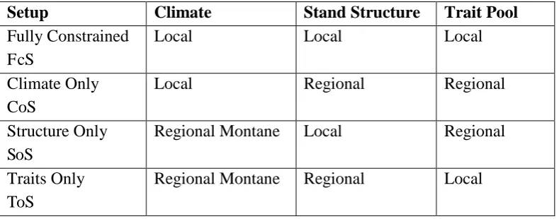
Finally, in the Fully constrained Set-up (FcS), we adopted the plot-specific set-ups of climate,

structure and traits (as outlines in the partial set-ups above) as our complete model.

Table S3.1: Summary of the different model setups used in this study. The Fully Constrained setup provides the most data demanding parameterisation where local scale climatic, functional diversity (traits) and stand structure data are required to predict GPP and NPP. The Climate Only setup requires knowledge of local climate and a regional description of trait diversity and stand structure, suggesting that climate is the most important predictor of GPP and NPP. The Structure Only setup

requires a detailed description of each stand‟s structure and regional level climate and traits data,

suggesting that stand structure is the most important predictor of GPP and NPP. The Traits Only

setup requires a detailed description of each plot‟s functional traits distributions and regional level

data of climate and stand structure, suggesting that functional diversity is the most important predictor of GPP and NPP.

Setup Climate Stand Structure Trait Pool

Fully Constrained FcS

Local Local Local

Climate Only CoS

Local Regional Regional

Structure Only SoS

Regional Montane Local Regional

Traits Only ToS

Regional Montane Regional Local

The predictive ability of the various model setups were quantified through standardised major axis

(SMA) regressions and estimation of root mean square error (RMSE in Mg C ha-1 y-1) between

observed and simulated GPP and NPP (see main text). In addition ordinary least square regressions

of simulated GPP and NPP with elevation were performed with the estimated slope ( OLS in MgC

ha-1 y-1 km-1) representing the sensitivity of each setup to changes in elevation. Here we present in a

19

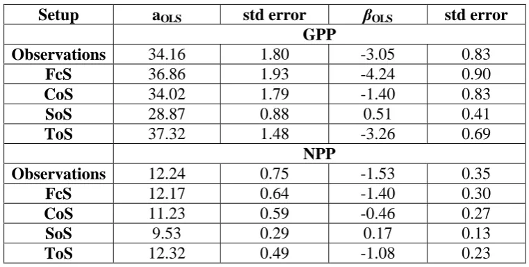
Table 3.2: Parameter estimates of the linear regression of observed and simulated GPP and NPP with elevation. Different model setups are used to explore the productivity sensitivity to climate, stand structure and functional traits. The sensitivity of GPP and NPP to elevation is summarised by the slope linear regression OLS (Mg C ha-1 y-1 km-1).

Setup aOLS std error OLS std error

GPP

Observations 34.16 1.80 -3.05 0.83

FcS 36.86 1.93 -4.24 0.90

CoS 34.02 1.79 -1.40 0.83

SoS 28.87 0.88 0.51 0.41

ToS 37.32 1.48 -3.26 0.69

NPP

Observations 12.24 0.75 -1.53 0.35

FcS 12.17 0.64 -1.40 0.30

CoS 11.23 0.59 -0.46 0.27

SoS 9.53 0.29 0.17 0.13

ToS 12.32 0.49 -1.08 0.23

20

S4. Tree size (D) distribution

Four theoretical distributions were used to describe the diameter at breast height (D) distribution in

all study plots. These distributions included the normal the log-normal, the Weibull and the

Gamma. We used the fitdistrplus R package to fit individual-tree D measurements to each

theoretical distribution and identify which of the four better described the observations. A summary

of these fits is provided in Table S4.1. The log-normal distribution better described the observations

and thus was used for initialising the model with an average stand structure (Fig S4.1).

Table S4.1: Parameters estimates (± standard error) of the four theoretical distributions fitted to individual-tree diameter measurements. The log-normal distribution provided the best fit, achieving the lowest AIC.

Theoretical Distribution Shape Scale or Rate AIC

Normal 19.686 (±0.116) 10.470 (±0.082) 61594

Log-normal 2.879 (±0.005) 0.424 (±0.003) 56245

Weibull 1.998 (±0.012) 22.288 (± 0.131) 59453

Gamma 5.128 (±0.077) 0.261 (±0.004) 57436

21

S5. Additional Simulation Exercises

A set of simulation exercises were applied, to explore the importance of temperature, light and

functional trait variation within our modelling framework. Below we describe these simulation

exercises and summarise some key findings.

Temperature Sensitivity

The importance of the effect of photosynthetic temperature sensitivity was explored following a

“leave-one-out” procedure that explored the ability of the model to simulate GPP and σPP patterns under three different model setups: 1) including both photosynthetic temperature sensitivity and

functional traits shifts along the gradient, 2) including only temperature sensitivity and 3) including

only functional trait shifts. In the first setup simulations were performed with both the temperature

sensitivity function (equation 8) and the plot-specific trait initialisation enabled. Thus the effects of

temperature on photosynthesis and the effects of environmental conditions (including temperature)

on species distribution and associated functional traits shifts along the gradient were taken into

account. In the second setup the temperature sensitivity function was enables but a gradient-wide

trait distribution was used, by-passing the effects of functional traits shift along the gradient. In the

third case, the photosynthetic temperature sensitivity function was disabled and only the local trait

distributions were used, accounting only for the effect of trait shifts.

The outputs of those simulations are summarised in Fig 2 and Table S5.1. Simulations including

photosynthetic temperature sensitivity and functional trait shifts along the gradient were too

sensitive to elevation changes, underestimating both GPP and NPP particularly at upland sites

[GPP: RMSE=9.75, OLS=-8.90, NPP: RMSE=2.86, OLS=-2.94] (Fig 2, Table SX). A similar model

behavior was observed even when only temperature sensitivity was included, assuming no

functional traits shift with elevation. However when trait values were allowed to vary with elevation

in accordance with observations and temperature sensitivity was excluded, the model illustrated the

best model performance [GPP: RMSE=3.25, OLS=-4.24, NPP: RMSE=0.99, OLS=-1.40]. We

defined this model setup, initialized with plot-specific solar radiation, stand structure and functional

traits data, as the fully constrained model setup (FcS). The FcS captures the broad gradient between

higher productivity in lowland sites and lower productivity in montane sites, suggesting that direct

temperature sensitivity could be excluded from our modelling framework (although it could still

matter through its effects on traits), and that across the gradient incoming radiation is the main

22

Table S5.1: Results of TFS performance under different setups. Bold values of the Pearson‟s correlation coefficient ( ) between field measurements and simulations indicate a statistical significant associations (p<0.05). In cases of statistical significant associations a SMA regression was fit and the slope SMA along with a 95% CI is reported. An adequate model performance is considered when SMA estimates include 1. RMSE (Mg C ha-1 y-1) between observations and simulations are also reported with lower values indicating a better model performance. The slope of an ordinary least square regression of simulated productivity with elevation OLS is also reported here to summarize the sensitivity of GPP and NPP with elevation. For comparison the estimated slope from observations for GPP is -3.05 (Mg C ha-1 y-1 km-1) and for NPP is -1.53 (Mg C ha-1 y-1 km-1).

Setup simulations- observations slope simulations- observations

( SMA)

RMSE simulations- observations slope simulations -elevation ( OLS)

GPP Temp +

Traits 0.82

0.89

(0.68 – 1.16) 9.75

-8.90 (±0.78)

Temp 0.90 0.84

(0.69 – 1.01) 7.88

-6.61 (±0.98)

Traits (FcS) 0.77 1.03

(0.93-1.14) 3.87

-4.24 (±0.90) NPP

Temp +

Traits 0.86

0.87

(0.70 – 1.09) 2.86

-2.94 (±0.26)

Temp 0.78 0.82

(0.68 – 1.00) 2.74

-2.18 (±0.32)

Traits (FcS) 0.90 1.01

(0.93-1.10) 0.99

-1.40 (±0.30)

The simulations used to explore for the importance of including a direct photosynthetic temperature

dependence were also tested against the ground-area corrected (rather than planimetric) estimates of

GPP and NPP (Fig S5.1a). Similar to Table S5.1 the best model performance was observed when

the photosynthetic temperature dependence was excluded and variation in functional traits between

plots was explicitly taken into account.

Table S5.1a: Results of TFS performance under different setups. Caption identical to Table S5.1 with observed GPP and NPP corrected for the slope of the plots, by dividing planimetric GPP and NPP with the cosine of the slope.

Setup simulations- observations slope simulations- observations

( SMA)

RMSE simulations- observations slope simulations -elevation ( OLS)

GPP Temp +

Traits 0.90

0.95

(076– 1.18) 7.56

23

Temp 0.93 0.89

(0.77 – 1.05) 5.75

-6.61 (±0.98)

Traits (FcS) 0.85 1.10

(1.00-1.20) 4.21

-4.24 (±0.90) NPP

Temp +

Traits 0.87

0.92

(0.76 – 1.11) 2.29

-2.94 (±0.26)

Temp 0.78 0.86

(0.72 – 1.04) 2.32

-2.18 (±0.32)

Traits (FcS) 0.90 1.07

(0.95-1.20) 1.47

-1.40 (±0.30)

24

Light Competition

To account for the importance of light competition, we compared the fully constrained model

simulations (FcS) that estimates individual-specific light availability with a model setup where light

competition was not explicitly simulated and all trees were assumed to receive the full amount of

available radiation. The overall model performance significantly decreased when light competition

was not taken into account, with the model substantially overestimating both GPP and NPP (Fig

S5.2 & Table S5.2). The above suggests that taking into account between-tree variation in light

availability is particularly important in order to capture variation in GPP and NPP along the tropical

forest elevation gradient.

25

Table S5.2: Comparison of model performance with and without light competition. Bold values of the Pearson‟s correlation coefficient ( ) between field measurements and simulations indicate a statistical significant associations (p<0.05). In cases of statistical significant associations a SMA regression was fit and the slope SMA along with a 95% CI is reported. An adequate model performance is considered when SMA estimates include 1. RMSE (Mg C ha-1 y-1) between observations and simulations are also reported with lower values indicating a better model performance. The slope of an ordinary least square regression of simulated productivity with elevation OLS is also reported here to summarize the sensitivity of GPP and NPP with elevation. For comparison the estimated slope from observations for GPP is -3.05 (Mg C ha-1 y-1 km-1) and for NPP is -1.53 (Mg C ha-1 y-1 km-1).

Setup simulations- observations slope simulations- observations

( SMA)

RMSE simulations- observations slope simulations -elevation ( OLS)

GPP

FcS - Light 0.77 1.03

(0.93-1.14) 3.87

-4.24 (±0.90)

FcS -No Light 0.78 1.56

(1.44-1.70) 16.44

-2.71 (±1.49) NPP

FcS - Light 0.90 1.01

(0.93-1.10) 0.99

-1.40 (±0.30)

FcS -No Light 0.35 5.38 -0.89

(±0.49)

Importance of elevation shifts in functional traits

In order to explore the effects of functional diversity along the tropical forest elevation gradient two

additional simulation exercises were performed, and compared with the FcS model setup. In the

first case individuals across all plots were set to have the same functional traits values, i.e. the

overall average LMA=113.8 (g m-2), NLm=21.00 mg g-1, PLm=1.42 (mg g-1) and W=0.57 (g cm-3).

This parameterisation is equivalent to having a single tropical tree PFT across the whole gradient,

and thus no species and/or traits turnover with elevation. In the second case, the plot average trait

values were assigned to all trees within a plot. This parameterisation is equivalent to have a plot

specific PFT and thus partially takes into account functional traits differences between plots

associated to species turnover with elevation. However within plot functional variation is not taken

into account.

The model performance statistics for these two exercises are compared with the FcS setup in table

S5.3 and Fig S5.3. Using a single PFT, i.e. overall average traits values substantially decreased the

predictive ability of the model. Furthermore, the decline of GPP and NPP with elevation ( OLS) was

not reproduced highlighting the role of functional traits shifts to drive the patterns of forest

26

account species and functional traits turnover with elevation a much better model performance was

achieved underlining the importance of species turnover for forest productivity along the study

gradient.

Table S5.3: Comparison of model performance with various level of functional diversity representation. Bold values of the Pearson‟s correlation coefficient ( ) between field measurements and simulations indicate a statistical significant associations (p<0.05). In cases of statistical significant associations a SMA regression was fit and the slope SMA along with a 95% CI is reported. An adequate model performance is considered when SMA estimates include 1. RMSE (Mg C ha-1 y-1) between observations and simulations are also reported with lower values indicating a better model performance. The slope of an ordinary least square regression of simulated productivity with elevation OLS is also reported here to summarize the sensitivity of GPP and NPP with elevation. For comparison the estimated slope from observations for GPP is -3.05 (Mg C ha-1 y-1 km-1) and for NPP is -1.53 (Mg C ha-1 y-1 km-1).

Setup simulations- observations slope simulations- observations

( SMA)

RMSE simulations- observations slope simulations -elevation ( OLS)

GPP FcS

Between and within plot functional trait variation

0.77 1.03

(0.93-1.14) 3.87

-4.24 (±0.90)

FcS – one PFT No functional trait

variation

0.69 0.92

(0.83-1.02) 4.08

-0.72 (±0.93)

FcS – nine PFTs Between plots functional

trait variation

0.85 1.00

(0.91 – 1.10) 3.55

-4.79 (±0.80)

NPP FcS

Between and within plot functional trait variation

0.90 1.01

(0.93-1.10) 0.99

-1.40 (±0.30)

FcS – one PFT No functional trait

variation

0.41 0.90

(0.76-1.07) 2.16

-0.24 (±0.31)

FcS – nine PFTs Between plots functional

trait variation

0.89 0.98

(0.90-1.07) 1.02

27