High Performance Fault-Tolerant
Solution of PDEs using the Sparse
Grid Combination Technique
Md Mohsin Ali
A thesis submitted for the degree of
DOCTOR OF PHILOSOPHY
The Australian National University
Some of the work in this thesis has been accepted for publication, or published jointly with others, see for example [Strazdins et al., 2016a,b; Ali et al., 2016, 2015, 2014]. Except where otherwise indicated, this thesis is my own original work.
Acknowledgments
This thesis, in fact, is a result of many people’s contributions. I may not be able to mention all of them, but my heartfelt appreciation goes to them for their valuable support and inspiration towards the accomplishment of my degree.
First and foremost I offer my sincerest gratitude to my supervisor Peter Strazdins. This thesis would not have been possible without his immense support, knowledge, guidance and patience. Thanks Peter for helping me happily sail through this aca-demic journey. I feel very lucky to have such an awesome supervisor like Peter.
I would also like to thank other members of my supervisory panel Alistair Ren-dell and Markus Hegland for helping me throughout my doctoral study.
I had the privilege of being able to contribute to a collaborative project (project LP110200410 under the Australian Research Council’s Linkage Projects funding sche-me) and would like to thank all members of the project for the many interesting dis-cussions. Specifically thanks to Brendan Harding for helping me during all the way of my doctoral study. He made things understand very easily and his informative discussions were very helpful. I would also like to thank Jay Larson for valuable suggestion and discussion about the research, and the remaining members of the project.
Fujitsu Laboratories of Europe Ltd was the collaborative partner in this project and I would also like to thank James Southern, Nick Wilson, and Ross Nobes for the interactions I had with them throughout the project and for hosting me for 7 weeks from 8 July to 31 August in the Hayes office in 2013 as a research intern.
I would also like to thank Christoph Kowitz, Ethan Coon, George Bosilca, Au-rélien Bouteiller, and Wesley Bland for valuable discussions.
All computations relating to this work were performed on Raijin, the peak system at the NCI Facility in Canberra, Australia, which is supported by the Australian Commonwealth Government. Thanks to the NCI Facility and its helpful staff.
I would also like to thank the Australian National University for helping me financially throughout the duration of my studies and stay in Australia.
I would also like to express my gratitude to all my fellow students for render-ing their friendliness and support, which made my stay in Australia very pleasant. Thank you Brian Lee and Sara Salem Hamouda for the helpful discussions.
I would also like to thank my friends in Australia especially Rifat Shahriyar, Wayes Tushar, Fazlul Hasan Siddiqui, Nevis Wadia, Sakib Hasan Siddiqui, little Afeef Ayman, little Abeed Ayman, Tofazzal Hossain, Presila Israt, little Taseen, Masud Rahman, Falguni Biswas, Adnan Anwar, Shama Naz Islam, little Arisha, Mirza Ad-nan Hossain, Ashika Basher, Shampa Shahriyar, SM Abdullah, Abdullah Al Mamun, Samia Israt Ronee, little Aaeedah Samreen, Rakib Ahmed, Surovi Sultana, Saikat
much more colorful with their company.
Abstract
The data volume of Partial Differential Equation (PDE) based ultra-large-scale scien-tific simulations is increasing at a higher rate than that of the system’s processing power. To process the increased amount of simulation data within a reasonable amount of time, the evolution of computation is expected to reach the exascale level. One of several key challenges to overcome in these exascale systems is to handle the high rate of component failure arising due to having millions of cores working to-gether with high power consumption and clock frequencies. Studies show that even the highly tuned widely used checkpointing technique is unable to handle the fail-ures efficiently in exascale systems. The Sparse Grid Combination Technique (SGCT) is proved to be a cost-effective method for computing high-dimensional PDE based simulations with only small loss of accuracy, which can be easily modified to provide an Algorithm-Based Fault Tolerance (ABFT) for these applications. Additionally, the recently introduced User Level Failure Mitigation (ULFM) MPI library provides the ability to detect and identify application process failures, and reconstruct the failed processes. However, there is a gap of the research how these could be integrated together to develop fault-tolerant applications, and the range of issues that may arise in the process are yet to be revealed.
My thesis is that with suitable infrastructural support an integration of ULFM MPI and a modified form of the SGCT can be used to create high performance robust PDE based applications.
The key contributions of my thesis are: (1) An evaluation of the effectiveness of applying the modified version of the SGCT on three existing and complex applica-tions (including a general advection solver) to make them highly fault-tolerant. (2) An evaluation of the capabilities of ULFM MPI to recover from a single or multi-ple real process/node failures for a range of commulti-plex applications computed with the modified form of the SGCT. (3) A detailed experimental evaluation of the fault-tolerant work including the time and space requirements, and parallelization on the non-SGCT dimensions. (4) An analysis of the result errors with respect to the num-ber of failures. (5) An analysis of the ABFT and recovery overheads. (6) An in-depth comparison of the fault-tolerant SGCT based ABFT with traditional checkpointing on a non-fault-tolerant SGCT based application. (7) A detailed evaluation of the infras-tructural support in terms of load balancing, pure- and hybrid-MPI, process layouts, processor affinity, and so on.
Contents
Acknowledgments vii
Abstract ix
1 Introduction 1
1.1 Problem Statement . . . 1
1.2 Scope and Contributions . . . 3
1.3 Thesis Outline . . . 4
2 Background and Related Work 5 2.1 Overview of Fault Tolerance . . . 5
2.2 Failure Recovery Techniques . . . 8
2.3 MPI-Level Fault Tolerance . . . 10
2.4 The Sparse Grid Combination Technique . . . 13
2.4.1 Classical Sparse Grid Combination Technique . . . 14
2.4.2 Fault-Tolerant Sparse Grid Combination Technique . . . 16
2.5 Related Work . . . 17
2.6 Summary . . . 19
3 Implementation Overview and Experimental Platform 21 3.1 Parallel SGCT Algorithm Implementation . . . 21
3.2 Hardware and Software Platform . . . 23
3.3 Fault Injection . . . 23
3.4 Performance Measurement . . . 24
4 Application Level Fault Recovery by ULFM MPI 27 4.1 Introduction . . . 28
4.2 Fault Detection and Identification . . . 28
4.2.1 Process Failure Detection and Identification . . . 28
4.2.2 Node Failure Detection and Identification . . . 29
4.3 Fault Recovery . . . 30
4.3.1 Faulty Communicator Reconstruction . . . 30
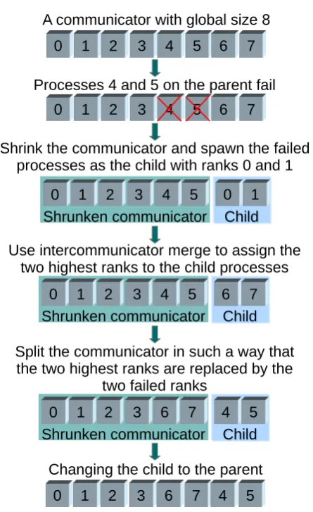
4.3.1.1 Spawning Based Recovery . . . 30
4.3.1.2 Shrinking Based Recovery . . . 32
4.3.2 Lost Data Recovery . . . 33
4.4 Experimental Results . . . 35
4.4.1 Experimental Setup . . . 35
4.4.2 Failure Identification and Communicator Reconstruction
Over-heads . . . 36
4.4.3 Failed Grid Data Recovery Overheads . . . 37
4.4.4 Approximation Errors . . . 39
4.4.5 Scalability . . . 39
4.5 Summary . . . 40
5 Fault-Tolerant SGCT with Applications 43 5.1 General Methodology for the SGCT Integration . . . 44
5.2 Fault-Tolerant SGCT with the Gyrokinetic Plasma Application . . . 45
5.2.1 Application Overview . . . 45
5.2.2 Implementation of the SGCT Algorithm for Higher-Dimensional Grids . . . 46
5.2.3 Modifications to GENE for the SGCT . . . 48
5.2.4 Experimental Results . . . 49
5.2.4.1 Experimental Setup . . . 50
5.2.4.2 Execution Time and Memory Usage . . . 50
5.2.4.3 Approximation Errors . . . 53
5.3 Fault-Tolerant SGCT with the Lattice Boltzmann Method Application . 53 5.3.1 Application Overview . . . 53
5.3.2 Modifications to Taxila LBM for the SGCT . . . 54
5.3.3 Experimental Results . . . 56
5.3.3.1 Experimental Setup . . . 56
5.3.3.2 Execution Time and Memory Usage . . . 56
5.3.3.3 Approximation Errors . . . 58
5.4 Fault-Tolerant SGCT with the Solid Fuel Ignition Application . . . 58
5.4.1 Application Overview . . . 58
5.4.2 Modifications to SFI for the SGCT . . . 59
5.4.3 Experimental Results . . . 60
5.4.3.1 Experimental Setup . . . 62
5.4.3.2 Execution Time and Memory Usage . . . 62
5.4.3.3 Approximation Errors . . . 62
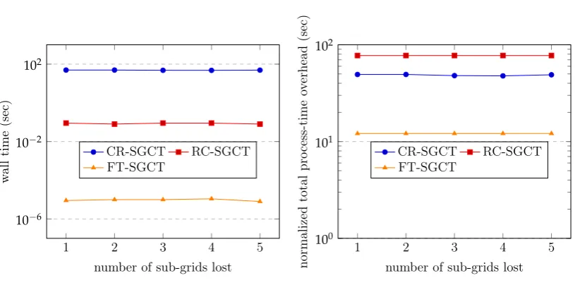
5.5 Failure Recovery Overheads . . . 63
5.5.1 Recovery Overheads for Shorter Computations . . . 63
5.5.2 Recovery Time Analysis for Longer Computations . . . 65
5.5.3 Overhead due to Computing Extra Grid Points . . . 67
5.5.4 Repeated Failure Recovery Overheads . . . 69
5.6 Summary . . . 70
6 Evaluation of the SGCT and Applications 71 6.1 Introduction . . . 71
6.2 SGCT Performance Analysis . . . 73
6.3 Load Balancing and Communication Profiles . . . 75
Contents xiii
6.5 Effect of Process Layouts on Performance . . . 79 6.6 Effect of Processor Affinity on Performance . . . 80 6.7 Summary . . . 81
7 Conclusion 83
7.1 Future Work . . . 85
A Process Recovery by ULFM MPI 87
List of Figures
2.1 Changes required in exascale systems. . . 6
2.2 Variation of MTTI with the number of CPUs. . . 7
2.3 The Sparse Grid Combination Technique. . . 14
2.4 A depiction of the 2D SGCT. . . 16
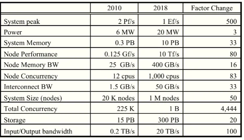
3.1 Message paths for the gather stage for the 2D direct combination method (not truncated) on a levell=5 combined grid. . . 22
4.1 Techniques of recovering failed processes. . . 31
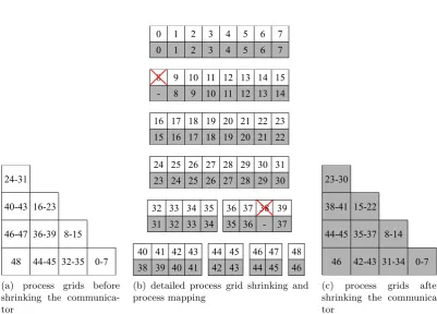
4.2 Process grid configurations of different sub-grids of the 2D FT-SGCT based applications with level l = 4 when the faulty communicator is shrunk as a recovery action. . . 32
4.3 Grid arrangements of the 2D SGCT with levell=4 solving the general advection problem to demonstrate different data recovery techniques. . 34
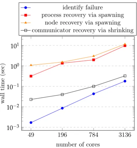
4.4 Times for generating the failure information and repairing the faulty communicator for the 2D SGCT solving the general advection problem. 36 4.5 Failed grid data recovery overheads of the 2D SGCT solving the gen-eral advection problem. . . 38
4.6 Approximation errors of the 2D FT-SGCT for the general advection solver. . . 39
4.7 Overall parallel performance of the 2D SGCT solving the general ad-vection problem with a single combination. . . 40
5.1 A demonstration of parallelization p =2 on the non-SGCT dimension Nz of GENE for the 2D SGCT. . . 47
5.2 Overall execution time and memory usage of the 2D FT-SGCT, 3D FT-SGCT, and the equivalent full grid computation with a single com-bination when there is no fault throughout the computation for the GENE application. . . 49
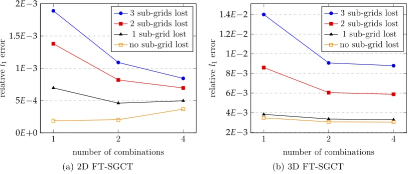
5.3 Approximation errors of the FT-SGCT based GENE application. . . 51
5.4 A comparison of the 2D full grid and level l =5 combined grid solu-tions for the GENE application. . . 52
5.5 Overall execution time and memory usage of the 2D FT-SGCT, 3D FT-SGCT, and the equivalent full grid computation with a single com-bination when there is no fault throughout the computation for the Taxila LBM application. . . 55
5.6 A comparison of the 2D full grid and level l= 5 combined grid solu-tions for the Taxila LBM application. . . 57 5.7 Overall execution time and memory usage of the 2D FT-SGCT, 3D
FT-SGCT, and the equivalent full grid computation with a single com-bination when there is no fault throughout the computation for the SFI application. . . 59 5.8 A comparison of the 2D full grid and level l= 5 combined grid
solu-tions for the SFI application. . . 61 5.9 Recovery overhead of a single occurrence of failures for shorter
com-putation for GENE. . . 63 5.10 Expected relative recovery overhead for longer computation for GENE. 66 5.11 Relative overhead required in the SGCT to achieve an ABFT. . . 68 5.12 Repeated ULFM MPI failure recovery overheads of the 2D FT-SGCT
with levell=5 applied to the GENE application over 64 cores. . . 69 6.1 Execution time of the average of ten combinations of the direct SGCT
in isolation. . . 72 6.2 Overall execution time of the general advection solver with the direct
SGCT running over 1024 time-steps (MPI warm-up time excluded). . . 73 6.3 An analysis of the TAU-generated load balancing of the 2D direct
SGCT computing the GENE application with2d_big_6input and a sin-gle combination (MPI warm-up time included). . . 74 6.4 An analysis of the IPM generated load balancing of the 2D direct SGCT
solving the general advection problem on level l = 11 with a single combination (MPI warm-up time excluded). . . 76 6.5 A comparison of the pure- and hybrid-MPI performance for the 2D
direct SGCT with levell =4 and a single combination (MPI warm-up time excluded). . . 77 6.6 A comparison of the performance due to different process layouts for
the 2D direct SGCT with level l = 4 and a single combination (MPI warm-up time excluded). . . 78 6.7 2D linear and block mapping of 32x4 process grid onto the cores of
Raijin nodes. . . 79 6.8 A comparison of the performance due to the linear and block
List of Tables
4.1 ULFM MPI performance to recover multiple process failures. . . 37 5.1 Execution time breakdown of the 2D FT-SGCT with parallelization p=
1 and levell=5 for the GENE application. . . 50 5.2 Execution time breakdown of the 2D FT-SGCT with level l=5 for the
Taxila LBM application. . . 56 5.3 Execution time breakdown of the 2D FT-SGCT with level l=5 for the
SFI application. . . 60 6.1 Parameters used in advection, GENE, Taxila LBM, and SFI experiments. 77 B.1 Parameters in testsuite/big/parameters_6 file used in GENE
ex-periments. . . 91 B.2 Parameters of Taxila LBM experiments fromtests/bubble_2D/input_data
andtests/bubble_3D/input_datafiles. . . 92
Chapter 1
Introduction
This thesis addresses the challenges and opportunities of achieving high performance fault tolerance of applications running on the upcoming exascale systems.
1.1
Problem Statement
Numerical solution of Partial Differential Equations (PDEs) is an important problem in computational science as PDEs are the basis of simulating all physical theorems1. The challenges that are encountered in all scientific simulations are thus essentially the same as solving the PDEs.
Today’s largestHigh Performance Computing(HPC) systems consist of thousands of nodes which are capable of concurrently executing up to millions of threads to simu-late the PDE based complex scientific problems within a feasible amount of time. The nodes within these systems are connected with high-speed network infrastructures to minimize communication costs [Ajima et al., 2009]. Significant effort is required to exploit the full performance of these systems. Extracting this performance is essen-tial in different research areas such as climate, the environment, physics and energy which all are characterized by the complex scientific models they utilize.
In the near future, besides exploiting the full performance of such large systems, dealing with component failures will become a critical issue. Since the failure rate of a system is roughly proportional to the number of nodes of the system [Schroeder and Gibson, 2006], current HPC systems consisting of thousands of nodes experience significant number of component failures. For instance, a 382-days study on the 557 Teraflops Blue Gene/P system with 163, 840 computing cores at Argonne National Laboratory showed that it experienced a failure (hardware) every 7.5 days [Snir et al., 2014]. Since the typical size of HPC systems is becoming larger as we approach exas-cale computing, the rate at which they experience failures is also increasing [Gibson
1 “. . . partial differential equations are the basis of all physical theorems. In the theory of sound
in gases, liquid and solids, in the investigations of elasticity, in optics, everywhere partial differential equations formulate basic laws of nature which can be checked against experiments.”
– Bernhard Riemann (1826-1866)
et al., 2007]. A study in [Snir et al., 2014] assumed theMean Time To Failure(MTTF) of an exascale system as 30 minutes.
Besides exascale computing, fault tolerance is also important in other areas, such as cloud computing, and scenarios, such as low power or adverse operating con-dition of the system. (a) In the large-scale and complex dynamic environments of cloud computing, there are several reasons such as expansion and shrinkage of the system size, update and upgrade of the system, online repairs, intensive workload on servers, and so on, that can induce failures and faults. The shrinkage of system com-ponents is required to exclude the faulty or high costly comcom-ponents of the system; whereas the expansion of system components is required to balance the server loads of the system. (b) In order to reduce the overall cost, sometimes system components (i.e., processors) are designed as very cheap to operate with low power consumption, which causes failures even with the moderate number of system components. More-over, adverse operating condition scenarios also cause failures. The common type of failures due to these scenarios is ‘bit-flips’ in memory or logic circuitry, which is termed assoftfaults.
The most commonly usedCheckpoint/Restart[Hursey et al., 2007] technique, which restarts the application from the recently checkpointed state in the event of failures, has several limitations to achieve fault tolerance in exascale systems. One of the key limitations is that a large amount of time required to write a checkpoint could be close to the MTTF. Although a parallelization of the checkpoint write and compu-tation/communication reduces the overall time, the key limitation is still in effect, together with a large amount of time required to read the checkpoint at restarts. Furthermore, the data volume of the future ultra-large-scale scientific simulations is expected to be increased, which in turn will increase the checkpoint write and read times.
pro-§1.2 Scope and Contributions 3
posed standard is very limited. Some of the work that is available assumes a fail-stop process failure model, i.e., a failed process is permanently stopped without recover-ing and the application continues workrecover-ing with the remainrecover-ing processes [Hursey and Graham, 2011]. However, continuation with only the alive processes is not sufficient for all applications. As for example, some applications do not tolerate a reduction of the MPI communicator size due to maintaining a strict load balancing and, thus, re-quire a recovery of the failed processes in order to finish the remaining computation successfully with balanced loads. Even the applications which are careless about load balancing require a major re-factoring effort in implementation if the communicator size is changed.
There appears to be an even greater lack of research on how to make existing, complex and widely used parallel applications fault-tolerant. In this thesis, we demonstrate how a general advection solver, and three existing real-world appli-cations (the GENE gyrokinetic plasma simulation, Taxila Lattice Boltzmann Method application, and Solid Fuel Ignition application codes) can be made fault-tolerant using ULFM MPI and a form of algorithm-based (application/user level) fault toler-ance obtained via modification of the Sparse Grid Combination Technique (SGCT). Our implementation and analysis include the restoration of failed processes and MPI communicators on either the existing or new (spare) nodes.
1.2
Scope and Contributions
There are different kinds of faults that may occur in a system. Based on the symp-toms and consequences of each category, different types of strategies to follow to handle them. The level of effort needed to identify and handle them may vary from one category to the other. Out of many categories, some common types of faults are transient (faults that occur once and then disappear), intermittent (faults that occur, then vanish again, then re-occur, then vanish), permanent(faults that continue to ex-ist until the faulty component is repaired or replaced), fail-stop(faults that define a situation where the faulty component either produces no output or produces output that clearly indicates that the component has failed), andByzantine(faults that define a situation where the faulty component continues to run but produces incorrect re-sults). Although it is desirable that a fault-tolerant technique will be able to handle all types of faults, but in practice, it is too hard to design and implement such a technique.
In this thesis, we are not handling all the above mentioned types of faults. The scope is narrowed down to handle only the permanent or fail-stop type of faults. More specifically, we are looking at the problem of recovering from the application process failures, caused by the hardware or software faults, from within the applica-tion.
The aim of this thesis under the stated scope is to:
fea-tures the preservation of communicator size and rank distribution after faults, the preservation of load balance, and either an exact or approximate data re-covery for the failed processes using the SGCT based general advection solver. • Detail how a scalable SGCT algorithm can be integrated not only into a general advection solver, but also into three existing and complex applications to make them highly fault-tolerant, and evaluate their effectiveness.
• Evaluate the capabilities of ULFM MPI to recover from a single or multiple real process/node failures for a range of complex applications.
• Perform a detailed experimental evaluation of the integrated applications in-cluding time and memory requirements, and parallelization on the non-SGCT dimensions.
• Perform an analysis of the result errors with respect to the number of failures, overhead due to computing some extra unknowns to achieve the fault tolerance, and an analysis of the recovery overheads. The latter includes a comparison with traditional checkpointing on a non-fault-tolerant SGCT based application. • Perform a detailed analysis of the SGCT algorithm and the applications in terms of load balancing, pure- and hybrid-MPI, process layouts, processor affin-ity, and so on.
1.3
Thesis Outline
The body of this thesis is structured around the key contributions outlined above. Chapter 2 provides an overview of fault tolerance and surveys relevant fault-tolerant literature. It provides more detailed background on previous fault tolerance tech-niques. Chapter 3 gives an overview of our implementation, and experimental plat-form.
Chapters 4, 5, and 6 comprise the main body of the thesis, covering the key contri-butions. Chapter 4 evaluates the effectiveness of ULFM MPI for the implementation of application level resiliency in the application. This includes a detailed implemen-tation guidelines for the detection, identification, and recovery of process and node failures with the ULFM MPI semantics. Chapter 5 evaluates the effectiveness of ap-plying the fault-tolerant SGCT on three different types of existing complex parallel applications. At the same time, this chapter also evaluates the application level re-covery overheads implemented by ULFM MPI on these applications, and compares these with the built-in checkpointing technique. Chapter 6 provides a detailed anal-ysis of the infrastructural support and the evaluation of applications on this infras-tructure with respect to combination algorithm’s scalability, load balancing, pure-and hybrid-MPI, process layouts, processor affinity, pure-and so on.
Chapter 2
Background and Related Work
This chapter provides background information on fault tolerance basics, failure re-covery techniques, MPI-level fault tolerance, the classical and fault-tolerant versions of the SGCT (computational model for the high-dimensional data processing), and related work to place the research contributions in context.
This chapter starts with a brief introduction to the field of fault tolerance in Sec-tion 2.1. SecSec-tion 2.2 describes failure recovery techniques and SecSec-tion 2.3 describes some MPI library based fault tolerance. A computational model (the SGCT) used for the high-dimensional data processing and its robust version are described in Sec-tion 2.4. An overview of the SGCT algorithm is presented in SecSec-tion 3.1. SecSec-tion 2.5 describes the research closely related to this thesis.
Sections 2.4 and 2.5 of this chapter are from the work published jointly with others as a part of the paper titled “Complex Scientific Applications Made Fault-Tolerant with the Sparse Grid Combination Technique” [Ali et al., 2016]. Section 2.4, of this chapter is also published jointly with others as a part of the paper titled “A Fault-Tolerant Gyrokinetic Plasma Application using the Sparse Grid Combination Technique” [Ali et al., 2015].
2.1
Overview of Fault Tolerance
The European Exascale Software Initiative (EESI) began their journey in the middle of 2010 with the hope of creating a common platform to tackle the issues that may arise in today’s and upcoming HPC systems. This initiative seems as a driving force of participating in a competition among different nations for building the next genera-tion supercomputers. For instance, in June 2011, Japanese K computer achieved the number one placing on the TOP5001list of the world’s fastest supercomputers, with a performance in excess of 10 petaflops (1016 floating point operations per second). But today, China’s Tianhe-2 replacing that positing, with a sustained performance of 33.86 petaflops, which is more than three times as powerful than K. This rate of in-crease puts HPC well on track to reach the next major milestone - exascale computing (1018flops) - by the end of the decade.
1http://www.top500.org/
Achieving this milestone will certainly require major changes to hardware and software technologies as shown in Figure 2.1. As it will be so hard to increase the clock frequency in the future, an exascale system is likely to have approximately one billion processing elements (cores) [Ashby et al., 2010]. Delivering these large number of elements will require more power. To keep it in an acceptable window, i.e., around 20 megawatts (MW) compared to 12.66 MW and 17.81 MW for K and Tianhe-2, respectively, it will require the development of novel architectures, most likely with increased heterogeneity. Similar to clock frequency, it is hard to increase the performance ofInput/Output(I/O) and memory systems compared to that of the processing elements. This will cause data movements on and off chip to dominate other operations, and create I/O bottlenecks on disk operations. This will require some software side solutions for maximizing local chip workload and placing part of the file system on the heterogeneous node.
Since the rate of component failures of a system is roughly proportional to the number of cores of the system [Schroeder and Gibson, 2006], an exascale system consisting of 1,000 times more cores than either the K computer (705,024 cores) or Tianhe-2 (3,120,000) will certainly suffer more frequent component failures. TheMean Time To Interrupt(MTTI), which is generally measured in days for today’s leading su-percomputers, will fall within the range of an hour in the exascale system due to this higher failure rate. A failure event analysis research at Los Alamos National Laboratory (LANL) with 140,000 interrupt events on 21 platforms shows remarkably similar trends of decreasing MTTI with the increase of number of cores in the system. 2DOE Exascale Initiative Roadmap, Architecture and Technology Workshop, San Diego, December,
[image:24.595.75.483.478.713.2]2009.
§2.1 Overview of Fault Tolerance 7
U N C L A S S I F I E D U N C L A S S I F I E D
Slide 25
Operated by the Los Alamos National Security, LLC for the DOE/NNSA LA-UR-07-4292/5853/6490
Failure at LANL: 140,000 Interrupt Events on 21
Platforms Show Remarkably Similar Trends
Sys
Data
Figure 2.2: Variation of MTTI with the number of CPUs3.
The results of this work presented in HPC-4 SDI/LCS seminar (October 10, 2007) are shown in Figure 2.2. Moreover, a study at the Oak Ridge National Laboratory showed that a 100,000-processor supercomputer with all its associated support systems could experience a failure every few minutes [Geist and Engelmann, 2002]. Current meth-ods for dealing with failures – often just re-run the application as failures are very unlikely to occur in two successive runs – will be unable to cope with this increase in the frequency of failures. An appropriate and efficient approach capable of handling such frequent failures on the large systems will be needed to successfully run the software on these systems.
The sources of such frequent failures include memory soft and hard errors; disks, file system or I/O node errors (disk reconstruction time); network connection faults (fibers, connectors, laser, etc.); resource exhaustion (memory, disc quota, etc.); Op-erating System/run-time/library bugs; hardware errors (power supply, fans, water valves, water connectors, water pipes, etc.); operators, system administrators, user er-rors; inconsistent maintenance, i.e., libraries update erer-rors; and so on. An experiment was carried out in LANL HPC systems over a period of a few years in [Schroeder and Gibson, 2010] to find out the root causes for system failures (both soft and hard). It is observed for these systems that hardware is the single largest source of faults, with 64% of all failures assigned to this category. Software is the second largest con-tributor, with 18% of all failures. It is also important to consider that the number of
failures obtained from the undetermined cause is significant. Total failures assigned to this category is 14%. A detailed root cause information reveals that CPU (42.8%) and memory DIMMS (21.4%) are the largest fraction of all hardware-related failures. For the software category, they are “other software” (30.0%), OS (26.0%), and parallel file system (11.8%). The largest fraction of all environment-related failures are power outage (48.4%), UPS (21.2%), power spike (15.1%), and chillers (9.8%).
The set of possible solutions to deal with these failures, as reported in [Snir et al., 2014], is divided into three categories: the hardwareapproach, the system approach, and theapplicationapproach.
The hardware approach will add additional hardware in an exascale system to deal with failures on the hardware level. Although this will require the least effort in porting current applications, it will incur additional power consumption in the system. Moreover, as the hardware in exascale system becomes more complex, the software will become more complex and hence error-prone. In this scenario, new complexities arise in the system due to the introduction of additional hardware.
In the system approach, fault tolerance is achieved by applying both the hardware and system software in such a way that the application code remain unchanged. Although it may be convincing that changing the system software is less costly than that of the hardware, this approach may add additional complexities in the system and, hence, may increase its energy consumption.
In the application approach, application code is extended to handle resiliency. No changes in hardware and system software are required. Since there are no additional costs and complexities due to extra hardware and system software, this approach may be suitable for exascale platforms. Moreover, application developers have more options to select the most appropriate resiliency strategy for their applications.
2.2
Failure Recovery Techniques
Some failure recovery techniques are as follows.
Checkpoint/Restart
§2.2 Failure Recovery Techniques 9
checkpointing just after restarting from the recent checkpoint.
Diskless checkpointing
Thediskless checkpointingapproach [Plank et al., 1998] is proposed to reduce the over-head of the Checkpoint/Restart approach. It stores a reduced volume of checkpoint state data onto compute nodes’ own memory without going to disk. It also needs some extra nodes to save a checksum of the memory checkpoint states so that it could be used to recover the memory checkpoints of the failed nodes. Although the per-formance of this technique is better than that of the disk-based Checkpoint/Restart method, there is a potentially significant memory I/O overhead to this method, espe-cially in memory intensive applications. Moreover, the number of additional nodes to store the checksum will grow in proportion to the number of nodes running the application.
Replication
The replication technique [Ferreira et al., 2011] is proposed to solve the problem of large overheads of the Checkpoint/Restart technique and to exempt the require-ments of storing checkpoints on memory of the diskless checkpointing approach. The idea of replication is that most applications leave some “wasted” spaces on the cluster machines on which they are executed. In order to efficiently use those spaces, multiple copies of the application are executed simultaneously. If there is any failure occurs, one of the replicated processes taking the charge of the original version of the application and the computation can continue onwards. This technique is applica-ble for some types of machines, especially those where the system utilization is not greater than 50%.
Message logging
The message loggingtechnique [Bouteiller et al., 2003] is proposed to reduce the roll-back overhead of the Checkpoint/Restart technique. It involves all processes to checkpoint their states without coordination and logging all communication oper-ations in a stable media. Thus, in case of any failures, this log is analyzed to restart the execution of only the crashed processes, rather than every processes, from the recent local snapshot, and establishing the same communication with the help of the saved communication log. However, the overhead of this technique is proportional to the communication volume of the application. A significant amount of penalty is added by this technique for all messages transferred even if there is no fault through-out the whole computation.
Task pools with reassignment
MapReduce algorithms [Dean and Ghemawat, 2008]. However, this method can be vulnerable to the failure of the manager node responsible for scheduling.
Proactive migration
The proactive migration technique [Chakravorty et al., 2006] is proposed to solve the problem of recomputing the affected tasks from the beginning of the task pools with reassignment technique. In order to avoid the recomputation, it predicts the failures in nodes before they really happen and moves the running applications away from them before the fault occurs. Theoretically, this would allow applications to run on fault-prone systems without any modifications. But practically, the performance monitoring of the nodes must occur sufficiently quickly that the application can be migrated before the failure does occur. Otherwise, it will not be applicable.
The success of the proactive fault tolerance solutions depends solely on the accu-rate prediction of the failures and the ranges of failures that it could cover. Prediction techniques used to achieve fault tolerance should incur less overhead, as well as, the work lost due to wrong prediction should be small. The state-of-the-art researches of this category is based on the data mining approaches [Gainaru et al., 2013].
Algorithm-Based or User Level Fault Tolerance
In theAlgorithm-Based Fault Tolerance(ABFT) technique [Huang and Abraham, 1984], numerical algorithms are modified to include methods for detecting and correcting errors. An extension of this is to develop new algorithms that are naturally resilient to faults. The major advantage of dealing with faults at the algorithm level is that the time-to-solution is roughly unchanged in the presence of faults. There may be an impact in terms of some loss of accuracy, but in many cases these are an acceptable compromise in order to guarantee a solution within a given time window.
Transactional Fault Tolerance
Transactional fault toleranceconcept is closely related to the distributed database sys-tems. This is used as a way of ensuring data consistency within distributed databases [Bernstein and Goodman, 1981]. Consistency will be achieved either by completing the submitted operation to the database successfully, or rolled back the database operation to a state prior to the operation was attempted. By performing updates in this atomic fashion, the database is protected from corruption in the case where the operation failed. With the popularity of concurrency in computing, transactional memory is introduced in [Herlihy et al., 1993] to assure the programmer that multi-ple concurrently running processes are not permitted writing on the same chunk of memory simultaneously. In order to achieve this goal, the ideas of transactions are currently considered into HPC, including a preliminary discussion of transactional fault tolerance in the MPI Standard.
2.3
MPI-Level Fault Tolerance
§2.3 MPI-Level Fault Tolerance 11
CoCheck
The CoCheck MPI [Stellner, 1996] is a combination of the Checkpoint/Restart and migration techniques. It uses a single process checkpointer which plays an important role of migrating the processes by saving the in-flight messages in a safe buffer and clearing the channel. This is achieved by exchanging a special message between the processes to indicate the clearance of the channel. If a process receives the special message, it assumes that there is no in-flight message left in the channel. Otherwise, it stores the special message in a special buffer as this is the in-flight message. When finally a process collects either the special or in-flight messages from all the processes destined to this process, it assumes that there is no ongoing message left in the channel. Hence, processes can now safely migrate with the checkpointer.
Starfish
TheStarfishMPI [Agbaria and Friedman, 1999] combines group communication tech-nology and the Checkpoint/Restart technique. This group communication technol-ogy allows the application to run without any disruption in the event that some of the nodes fail. Failure recovery is achieved by recomputing the part of the appli-cation which are disrupted due to failures. Recomputation is done either from the beginning, or from the recent checkpointed state by the Checkpoint/Restart tech-nique. This is usually performed on the extra nodes added to the application by the Starfish on-the-fly. This run-time node adding feature allows Starfish to migrate the application processes from one node to another node with the assistance of the Checkpoint/Restart technique. Moreover, Starfish has the capability of performing both the application independent and application dependent fault tolerance.
MPI-FT
MPI-FT [Louca et al., 2000] is a fault-tolerant version of MPI. It performs failure recovery by means of reassigning tasks to the replacements for the dead processes. A detection technique is used for the detection of process failures. A centralized monitoring process (called the Observer), responsible for notifying the failure event to the rest of the alive processes, performs the recovery action. There are two modes of the recovery action. The first one performs distributed buffering of message traffics on each process. When the Observer detects process failures, it performs recovery by resending buffered messages from all the processes to the replacement processes, those are originally destined for the dead ones. The second one is based on the idea of centrally storing every message traffics by the Observer, and resend these to the replacements for the dead processes.
be synchronized.
MPICH-V
MPICH-V[Bosilca et al., 2002] is a fault-tolerant version of MPI combining features from the uncoordinated Checkpoint/Restart and message logging techniques. With the MPICH-V run-time support, any application written in standard MPI could be made fault-tolerant. The key idea is that a Dispatcher coordinates the whole appli-cation execution by periodically collecting ‘’alive” messages from all the nodes, and at the same time keeps records of all the communications in stableChannel Memories (CM). In addition to this, every node checkpoints their task images to a Checkpoint Server (CS). If any ‘’alive” message is not received for a certain period of time, the Dispatcher assumes that the particular node is dead, and restarts the execution from the point of failure with the support of the CS. By this time, if that faulty node re-joins the system, the duplicate instance removal is managed by the CM. Moreover, network connection management for the alive and dead nodes is achieved by the CM.
The service provided by MPICH-V seems to be automatic and transparent to an application developer. However, periodic monitoring of all the nodes and periodic checkpointing of all the nodes task images to stable storages incur a large overheads to the application.
FT-MPI
FT-MPI[Fagg and Dongarra, 2000] offers a number of options for automatic process-level fault tolerance within the MPI library itself. This is achieved by simply calling a new communicator creation function, such asMPI_COMM_DUPorMPI_COMM_CREATE, in the application, with almost no impact on the user code.
FT-MPI provides the following three types of recovery modes to chose from by an application developer.
• The first recovery mode is SHRINK, which builds a new communicator exclud-ing the failed processes and shrink the communicator size. Although the alive processes are ordered in the communicator, but for some applications where computation depends on the consistent values of the local ranks, this shrinkage could cause problems.
• The second recovery mode is BLANK. This is similar to SHRINK in the sense that all the failed processes are removed from the reconstructed communica-tors. However, without shrinking the communicator size, it replaces them with invalid process ranks. Although communication with the invalid ranks causes error, but those are left for future development to replace with new processes so that there is no disruption in inter-process communication.
§2.4 The Sparse Grid Combination Technique 13
processes. However, for the other communicators they must be reconstructed manually.
Initially, FT-MPI was built on the top of Parallel Virtual Machine (PVM) due to the unavailability of proper MPI run-time. Later, the HARNESS run-time [Fagg et al., 2001], originally implemented in Java, was rewritten in C to be used for FT-MPI. This run-time provides important features such as the ability to create new processes, examining their health, and monitor the status of all processes executing the appli-cation.
Although FT-MPI had lots of functionalities to provide the fault tolerance sup-port, it was never adopted into the MPI standard due to the lack of standardization, and its development was discontinued.
ULFM MPI
User Level Failure Mitigation(ULFM) [Bland, 2013a] MPI can be considered as an at-tempt of resolving the non-standardization issue of FT-MPI. The MPI Forum’s Fault Tolerance Working Group began the implementation of standard fault-tolerant MPI by introducing a new set of semantics on the top of the existing standard MPI li-brary [Bland, 2013b]. Semantics of the draft standard include the detection and identification of process failures, propagating the failure information within the alive processes in the faulty communicator, and so on. Usually process failures are de-tected by checking the return code of the collective communication routines. With the run-through stabilization mode [Fault Tolerance Working Group] of ULFM MPI, surviving processes can continue their operations while others fail. The alive pro-cesses can form a fully operational new communicator without getting any disrup-tion from the dead processes. It is also possible to create the replacement processes for the failed ones to recover the original communicator. Based on the requirements of the application, either the local or global recovery is also possible.
ULFM MPI supports the coordinated Checkpoint/Restart without modification. It is also possible to create the uncoordinated Checkpoint/Restart without requiring the application to restart entirely. The implementation of message-logging techniques and transactional fault tolerance on the top of ULFM MPI also achieves some bene-fits. Furthermore, ABFT techniques could be easily integrated with ULFM MPI. For details, see Chapter 4.
2.4
The Sparse Grid Combination Technique
Figure 2.3:The Sparse Grid Combination Technique. Gi,j,GcI, andGf represent the sub-grid,
sparse or combined grid, and full grid equivalent to the sparse grid, respectively, for the 2D
case. A distinct set of processes computes each Gi,j in parallel via domain decomposition.
Solutions on Gi,j are linearly combined to approximate the solution of Gf on GcI. Multiple
processes are also running onGcI.
2.4.1 Classical Sparse Grid Combination Technique
The Sparse Grid Combination Technique(SGCT) [Griebel, 1992; Griebel et al., 1992b] is a method of approximating the sparse grid solution which in turn approximates the full grid solution. Instead of solving the PDE on a full isotropic grid, it is solved on a set of smallanisotropicregular grids referred to assub-gridsorcomponent grids. Finally, solutions on these sub-grids are linearly combined to approximate the solution on the sparse grid (or, in this context, called combined grid). For the 2D problem, this technique is illustrated in Figure 2.3. This technique can be applied in principle to any PDE, but sufficient smoothness of the solution is required for high accuracy.
Suppose that each sub-gridGi,j in 2D has(2i+1+1)×(2j+1+1)grid points with
a grid spacing of hx = 2−i−1 and hy = 2−j−1 in the x and y directions,
respec-tively, wherei,j ≥ 0. With a 2D domain, the grid points ofGi,j are {(2ix+1,
y
2j+1)|x =
0, 1,· · · , 2i+1,y = 0, 1,· · · , 2j+1}. In the more general case, the index space for the grids will be some finite I ⊂Nd, where d is the grid dimension, and the set of grids
of interest can be denoted by{Gi,i∈ I}. Ifui denotes the approximate solution of a
PDE onGi, the combination solutionucI on gridGcI generally takes the form ucI =
∑
i∈I
ciui, (2.1)
where the ci ∈ R are the combination coefficients. Clearly, the accuracy of the
§2.4 The Sparse Grid Combination Technique 15
ifi+j= l−1 andci,j = −1 ifi+j=l−2. This provides the combination formula ucI =
∑
i+j=l−1
ui,j−
∑
i+j=l−2ui,j. (2.2)
Note that levell=3 for the classical SGCT shown in Figure 2.3.
The computation on sub-grids Gi and their combinations are performed in the
following way. At a time-stepti, PDE instances are computed (solved) concurrently
on each Gi with the corresponding grid points and spacing. This is continued for T successive time-steps with step-size ∆t. After that, all the solutions ui on Gi are
assembled to get the combined solutionucI on gridGcI for time-stepti+T. Then,ucI is
projected for all the sub-gridsGi with the properly adjusted weights, and the whole
process is repeated withti = ti+T.
In this thesis, we use the notion of singleandmultiplecombinations. If the above mentioned process is not repeated, we call it a single combination. In this case, T becomes the same as the total number of time-steps applied to compute the solution on the equivalent full gridGf, sayT0. On the other hand, with multiple combinations, the process is repeated for multiple times, but with T< T0. If we want to performn repeated combinations, thenTbecomes T0/n.
In this thesis, we also use so-called ‘truncated’ combinations [Benk and Pfluger, 2012], where, for the 2D case, each sub-grid has (2i+1+1)×(2j+1+1) points, for some (i,j)≥ (i0+1−l,j0+1−l). This avoids the problem of minimum dimension size imposed by some applications. Furthermore, it allows us to avoid the use of highly anisotropic grids (e.g. G0,l−1), which have been known to contribute least to-wards the accuracy of the sparse grid solution or cause convergence problems [Benk and Pfluger, 2012], and enabling us to concentrate process resources on more accu-rate sub-grids. In this context, we use a different notion of level to that described previously, which describes how much smaller the sub-grids are relative to some full grid Gi0,j0. In particular, a levell ≤ min{i0+1,j0+1}in this context consists of
sub-grids from the index set
I =
(
(i,j): (i
0+1−l,j0+1−l)≤(i,j) i0+j0−l≤i+j≤i0+j0+1−l
)
. (2.3)
Similarly, for the 3D SGCT with a reference full gridGi0,j0,k0, a levell≤min{i0+1,j0+
1,k0+1}consists of sub-grids from the index set
I =
(i,j,k):
(i0+1−l,j0+1−l,k0+1−l)≤(i,j,k) i+j+k≤i0+j0+k0+2−2l
i+j+k≥i0+j0+k0−2l
. (2.4)
Two levels of parallelism are achieved in the SGCT computation. Firstly, different sub-grids are computed in parallel. Secondly, each sub-grid, Gi, is assigned to a
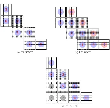
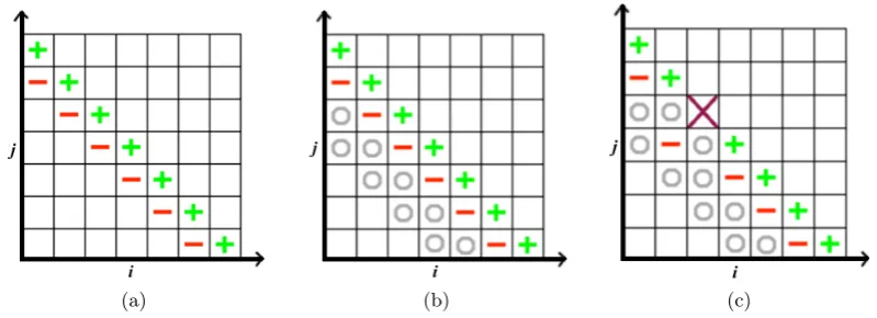
(a) (b) (c)
Figure 2.4: A depiction of the 2D SGCT. ‘+’, ‘–’, and ‘o’ on a sub-grid denotes the computed solution on that sub-grid is added, subtracted, and ignored, respectively, on the combined solution. ‘x’ on a sub-grid denotes the solution on that sub-grid is lost and ignored in the combination. (a) Classical SGCT, (b) fault-tolerant SGCT with extra smaller sub-grids on two lower layers (marked with ‘o’) and without any loss of sub-grid solution, and (c) fault-tolerant
SGCT in the event of a lost solution on sub-gridG2,4.
In contrast to the full grid approach which consists of O(h−l d) grid points, the SGCT consists of only O(h−1l (log2h−1l )d−1) grid points, where hl = 2−l denotes
the employed grid spacing with level l, and d is the dimension. The accuracy of the solution obtained from the SGCT deteriorates only slightly from O(hrl) to O(hrl(log2h−1l )d−1)for a sufficiently smooth solution of orderrmethods [Garcke and Griebel, 2000].
2.4.2 Fault-Tolerant Sparse Grid Combination Technique
A fault-tolerant adaptation of the SGCT has been studied in [B. Harding and M. Hegland, 2013]. In this thesis, we refer to this adaptation asFault-Tolerant SGCT (FT-SGCT). It is observed that the solution on even smaller sub-grids can be computed at little extra cost and that this added redundancy allows combinations with alternative coefficients to be computed. When a process failure affects one or more processes involved in the computation of one of the larger sub-grids, the entire sub-grid is discarded. In the event that some sub-grids have been discarded one must modify the combination coefficients such that a reasonable approximation is obtained using solutions computed on the remaining sub-grids. In 2D, this involves findingci,j for
formula (2.1) for which ci,j = 0 for eachui,j which was not successfully computed.
For a small number of failures this is typically done by starting with formula (2.2) and subtracting hierarchical surplus approximators of the form ui0,j0−ui0−1,j0−ui0,j0−1+
ui0−1,j0−1 such that the undesired ui,j drop out of the formula whilst introducing
§2.5 Related Work 17
coefficients is described in [Harding et al., 2015].
For the 2D fault-tolerant SGCT computations in this thesis, two extra layers (or diagonals) of sub-grid solutions ui,j are computed satisfying i+j = l−3 and i+j= l−4. These two extra layers of sub-grids have levels l−3 and l−4, respec-tively. During fault-free operation these extra sub-grid solutions are not used in the combination formula (2.2). Rather, all sub-grid solutions ui,j with i+j = l−1 and i+j=l−2 are used. However, if any of the sub-grid solutionsui,j withi+j=l−1
ori+j= l−2 do not complete due to a fault, some of the extra and remaining unaf-fected sub-grid solutionsui,jare used in an alternate combination of the form (2.1) so
that the combination gives the best result. An example of the default combination, an alternative leaving extra sub-grids unused, and an alternative using one of the extra sub-grids is depicted in Figure 2.4. For the 3D fault-tolerant SGCT computations in this thesis, one additional layer (or diagonal) of sub-grids with levell−4 was com-puted (with the 3 layers l−1, l−2, and l−3 necessarily computed for the default combination).
In this thesis, we also use ‘truncated’ combinations [Benk and Pfluger, 2012] for the FT-SGCT. The lower limit of formula (2.3) is changed to achieve this when extra layers are added, e.g. i0+j0−l−2≤i+jfor two extra layers. Similarly, lower limit of formula (2.4) could be updated to achieve the 3D FT-SGCT.
2.5
Related Work
This thesis work lies at the intersection of four active research and development ar-eas – parallelization of the SGCT, recovery of process and node failures with ULFM MPI, Algorithm-Based Fault Tolerance (ABFT) technique, and evaluation of the effec-tiveness of applying the SGCT to the GENE plasma micro-turbulence, TaxilaLattice Boltzmann Method(Taxila LBM), andSolid Fuel Ignition(SFI) application codes. Below we summarize and contrast work most closely related to ours.
A technique for replacing only a single failed process in the communicator and matrix data repair for a QR-Factorization problem was proposed in [Bland, 2013b]. Process failure was handled by ULFM MPI, and data repair was accomplished by using a reduction operation on a checksum and remaining data values. The author analyzed the execution time and overhead on a fixed number of processes in the presence of a single process failure. A detailed performance analysis of the recovery mechanism for multiple process failures, however, was not presented. Nor was the technique applied to a varying number of processes in other realistic parallel appli-cations. A detailed performance evaluation of different ULFM MPI routines used to tolerate process failures was found in [Bland et al., 2012].
samples affected by failures. The periodic communication/reduction is likely to be costly across multiple nodes, and the experimental results relating to multiple nodes were not provided. Reconstruction of the faulty communicator was not considered, nor was data recovery implemented.
Local Failure Local Recovery(LFLR) was proposed in [Teranishi and Heroux, 2014]. It inherited the idea from diskless checkpointing [Plank et al., 1998] in which some spare processes accommodated a space for data redundancy and local checkpointing. This allows an application developer to perform a local recovery without disrupting the execution of whole application when a process fails. The idea is to split the orig-inal communicator into several group communicators and dedicate a spare process for each group to store the parity checksum of the corresponding group. In the event of a single process failure, the corresponding spare process replaces the failed one with ULFM MPI, and recover the lost data locally from the local memory check-sum. It requires local checksum to be updated periodically, which seems to be costly. Spare processes are used in the LFLR approach to handle only a single process fail-ure. In this thesis, extra processes are also used for a small amount of redundant computations, but we are able to tolerate multiple process/node failures.
A customized run-time based simplified programming model calledFault-Tolerant Messaging Interface(FMI) was designed and implemented in [Sato et al., 2014] to im-prove the resilience overheads of the existing multi-level checkpointing method and MPI implementations. The semantics needed to write applications were similar to MPI, but the resiliency of applications was ensured by the FMI interface. Scalable failure detection with the help of a log-ring overlay network, fast in-memory check-pointing on spare nodes, and dynamically allocating spare compute resources in the event of failures were proposed. Although the main objective of providing resiliency to applications is the same, we are applying an ABFT for the approximate recovery of multiple failures, rather than the exact recovery through diskless checkpointing. Our failure detection and process recovery techniques are also different.
Early work in the parallelization of the SGCT for Laplace’s equation and the 3D Navier-Stokes system were reported in [Griebel, 1992] and [Griebel et al., 1996], respectively. However, fault-tolerant issues were not considered.
ABFT techniques for creating robust PDE solvers based on the FT-SGCT were proposed in [Larson et al., 2013a; B. Harding and M. Hegland, 2013]. The proposed solver can accommodate the loss of a single or multiple sub-grids. Grid losses were tolerated by either deriving new combination coefficients to excise a faulty sub-grid solution or approximating a faulty sub-grid solution by projecting the solution from a finer sub-grid. This work, however, was implemented using simulated, rather than genuine, process failures. Furthermore, this work assumed that an application process failure is followed by a recovery action such as communicator repair, but did not actually implement such a mechanism. Finally, the results used a simple advection solver, whereas the work in this thesis uses real-world and pre-existing applications.
out-§2.6 Summary 19
puts written to data files that were subsequently combined to compute the SGCT solution. Complimentary work to ours on load balancing of GENE sub-grid in-stances and an alternative hierarchization based implementation of the SGCT has been reported in [Heene et al., 2013] and [Hupp et al., 2013], respectively. None of these aforementioned efforts has investigated the fault-tolerant possibilities of the SGCT for this application, nor have they implemented any alternative fault-tolerant techniques.
The effectiveness of ABFT by applying the FT-SGCT to GENE was analyzed in [Parra Hinojosa et al., 2015; Pflüger et al., 2014]. An analysis of solution accura-cies in the event of several sub-grids lost, and the overhead of computing redundant smaller sub-grids were presented there. The load balancing implemented there was from the developed load model from amaster-slaveparallelism model. In this thesis, we contribute the tolerance of real process and node failures with ULFM MPI, which was absent there. Moreover, we provide a load balancing scheme on a globalSingle Program Multiple Data(SPMD) parallelism model and show how several SGCTs could be applied to the non-SGCT dimensions concurrently4.
2.6
Summary
This chapter introduces key background material. We discuss the importance of fault tolerance, the reasons behind the failure of supercomputer nodes, an overview of some failure recovery techniques, including fault tolerance techniques implemented on the top of the MPI library. We discuss the SGCT and a fault-tolerant version of the SGCT, which provide necessary background for the key contributing thesis chapters. We further discuss some research work closely related to the contributions of this thesis. Before we move to the primary contributions of the thesis, we next give an overview of our implementation, and experimental platform.
4The concept of non-SGCT dimensions arises from the scenario where the total number of
Chapter 3
Implementation Overview and
Experimental Platform
This chapter presents an overview of our implementation, hardware and software platform, fault injection technique, and measurement methodologies that we use throughout the evaluations presented in this thesis.
3.1
Parallel SGCT Algorithm Implementation
An implementation of thedirectSGCT algorithm is used in this thesis. The key idea of this algorithm is to perform a scaled addition of part of each sub-grid’s solution ui inPi to Pcto get the combined (or sparse) grid solution ucI.
With the direct SGCT algorithm, each PDE instance whose solution isuiis run on
a distinct set of processes denoted by Pi and is arranged in a logicald-dimensional
grid. The algorithm consists of first a gather stage, where each process in Pi sends
its portion of ui to each of the corresponding (in terms of physical space) processes
in a logical d-dimensional grid Pc to be scaled added into uc
I. This is illustrated
in Figure 3.1. The portion of ui is selected based on the local to global mapping
of processes in each d dimension from Pi to Pc. Suppose, a 2D process grid Pi is
represented by {Pix,Piy}, and Pc by {Pxc,Pyc}. If Pix = Pxc and Piy = Pyc, then the whole solution ui is scaled added intoucI (initially ucI is empty) with an exact mapping of
processes. Otherwise, solutionui is split into Pxc Px
i and Pc
y
Piy parts inxandydimensions,
respectively, and then scaled added each chunk of ui into ucI. In this case, each
process inPix and Piy is mapped into Pxc Px
i and Pc
y
Piy processes of P c
x and Pyc, respectively.
Finally, each process in Pc then gathers the|I|versions of each point of the full grid (using interpolation where necessary), and performs the summation according to formula (2.1) to get the combined (or sparse) grid solution uc
I, which can be used as
an approximation to the full grid solution. The use of interpolation in turn requires that a ‘halo’ of neighbouring points (in the positive direction, for our implementation) have been filled by a halo exchange operation by each process in eachPi and is also
sent in the gather stage. For reasons of efficient resource utilization, Pc is made up
Figure 3.1: Figure 4 from [Larson et al., 2013b]. Message paths for the gather stage for the
2D direct combination method (not truncated) on a levell=5 combined grid. The combined
grid and component grid (3,3) have 2×2 process grids, all others have 2×1 or 1×2 process
grids.
Similarly, in the scatter stage, a reverse mapping of processes from Pc to Pi is
done to scatter a down sample ofucI toPi, iteratively, for eachi∈ I.
Further details on the algorithm using a full grid representation of the combined gridGcIare available in [Strazdins et al., 2015]. An improved version of this algorithm, where a partial sparse grid, rather than a full grid, representation of Gc
I is used to
perform an efficient interpolation onGcI, is available in [Strazdins et al., 2016b]. We used this improved version of the algorithm in this thesis, except where otherwise indicated.
In terms of load balancing, we used a simple strategy to balance the loads among the processes. The same number (p0 ∈ N) of processes is allocated on each of the distinct set of processes Pi for each sub-grid on the uppermost diagonal (i.e., for the
2D case, eachGi,jwithi+j=l−1) in the grid index space. Each sub-grid on the next
lower diagonals (i.e., for the 2D case, each Gi,j with i+j = l−2, i+j = l−3, and i+j= l−4) is allocated dp0/2e,dp0/4e, anddp0/8eprocesses, respectively. Details are discussed and analyzed in Section 6.3 of Chapter 6.
A failure of computing nodes or application processes causes the loss of some processes on some gridsGi. This is handled as follows. Before the SGCT algorithm
is applied, the loss of any processes inPi is detected using ULFM MPI (see Chapter 4
§3.2 Hardware and Software Platform 23
permanent). Otherwise, replacements are created on a spare node. Following the reconstruction of communicators, an alternate combination formula (see Section 2.4) is derived which sets a combination coefficient ofci =0 for the lost sub-grid solutions ui. Note that this formula can be computed on all current processes. In this case,
the gather of ui on the replaced Pi and Pc is not performed. Note that the replaced Pi andPc do participate in the scatter operation so that they are populated with the
combined data to replace the lost data.
3.2
Hardware and Software Platform
All experiments were conducted on the Raijin cluster managed by theNational Com-putational Infrastructure(NCI) with the support of the Australian Government. Raijin has a total of 57,472 cores distributed across 3,592 compute nodes each consisting of dual 8-core Intel Xeon (Sandy Bridge 2.6 GHz) processors (i.e., 16 cores) with In-finiBand FDR interconnect, a total of 160 terabytes (approximately) of main memory, and 10 petabytes (approximately) of usable fast filesystem operated by the x86_64 GNU/LinuxOS [Cit].
We used git revision icldistcomp-ulfm-46b781a8f170of ULFM MPI (as of 13 December 2014) under the development branch 1.7ft of Open MPI for our experi-ments. The parameters for the collective communications formpirunwere set tocoll
tuned,ftbasic,basic,self. The value of the MCA parameter
coll_ftbasic_met-hod was set to 1 to choose the ‘Two-Phase Commit’ as an agreement algorithm for the failure recovery. The ‘Log Two-Phase Commit’ option was more scalable than the used one, but could not be used in our experiments due to its instability. All the source code (including ULFM MPI) were compiled withGNU-4.6.4compilers using the optimization flag -O3. The versions of PETSc [Balay et al., 2014] and MPI were
petsc-3.5.2 and openmpi-1.4.3 (used for the simulations with non-real process failures), respectively.
Although InfiniBand interconnect was used in the Raijin cluster, the BTL compo-nent TCP was used while executing applications. Due to an issue in icldistcomp-ulfm-46b781a8f170 distribution of ULFM MPI, the execution of applications re-ported an warning that there was an error initializing the OpenFabrics device. This issue has been fixed in the recently released ULFM MPI version 1.0 and subsequent commits, but considering the wastage of lots of CPU hours, we did not repeat the experiments.
3.3
Fault Injection
where <PID> was the application process identification number (either a single or multiple) extracted by the ps -A | grep <executable_application_name> com-mand from the comcom-mand-line when the application was in execution. The processes were also killed repeatedly (not at a single time) to analyze the repeated failure re-covery performance of the application.
3.4
Performance Measurement
The IPM profiling tool [Wright et al., 2009; IPM] was used to report the total mem-ory usage of the applications. The deallocation of memories in the application code was disabled to generate the memory usage reports. The reason behind this ap-proach was that a mixture of different programming languages were used to create the SGCT based applications. As for example, the SGCT was implemented in C++, but the applications integrated with it was implemented either in FORTRAN or in PETSc [Balay et al., 2014] (details in Chapter 5). With these interoperable program-ming languages, the best way of generating memory reports by the IPM tool was unclear. Thus, theMPI_Pcontrol()function was called in the main C++ program to create a code region consisting of computing the grids and combining the sub-grids’ solutions to generate the memory usage reports. Moreover, to save CPU hours, the number of time-steps was set to 1 or as minimum as possible in this context.
Both the TAU [Shende and Malony, 2006] and IPM [Wright et al., 2009; IPM] profiling tools were used to analyze the load balancing and communication profiles. The ways of generating profiles for computing the sub-grids and performing the combination as a whole, and in isolation were a little bit different. For the former case, the sequence of instructions were: (1) setting a barrier (by the MPI_Barrier()
function call) before the computation of sub-grids, (2) start a code region by the
MPI_Pcontrol() function call function, (3) compute the sub-grids, (4) perform the combination, and (5) end the code region by theMPI_Pcontrol()function call. For the latter case, the sequence of instructions were: (1) setting a barrier before the com-putation of sub-grids, (2) start a code region by the MPI_Pcontrol() function call, (3) compute the sub-grids, (4) end the code region by theMPI_Pcontrol()function call, (5) setting a barrier before performing the combination, (6) start a code region by the MPI_Pcontrol()function call, (7) perform the combination, and (8) end the code region by theMPI_Pcontrol()function call.
MPI_Wtime() function was used to measure the execution performance of the
applications. In order to measure the whole application running time in isolation, barriers were placed in the same way as they were used for the analysis of the load balancing and communication profiles. Throughout this thesis, ‘sec’ and ‘msec’ rep-resent seconds and milliseconds, respectively.
Approximation error was represented by the relative l1 error of the combined field. It was computed by ku0−uk1
§3.4 Performance Measurement 25
![Figure 3.1: Figure 4 from [Larson et al., 2013b]. Message paths for the gather stage for thegrid and component grid (3,3) have 22D direct combination method (not truncated) on a level l = 5 combined grid](https://thumb-us.123doks.com/thumbv2/123dok_us/8205698.262039/40.595.156.400.108.369/figure-figure-message-thegrid-component-combination-truncated-combined.webp)