Application of Data Mining Techniques to Examine Quality of Water

(1)

International Journal of Innovative Technology and Exploring Engineering (IJITEE) ISSN: 2278-3075, Volume-8 Issue-5S March, 2019

Abstract: Water is one of the most used natural resources. Increase in content of harmful chemicals is one of the main reasons which will affect quality of water. Continuous monitoring and early forecasting can help us in maintaining quality of water. Data mining is one of the most efficient techniques that can effectively perform this operation. It is the process to discover interesting information from even large amounts of data. In this paper we are going to make use of R tool to perform data mining for water samples.

Keywords: Multiple linear regression; Randomforest; RegressionTree; Model evaluation;

I. INTRODUCTION

High frequency of certain algae in water leads to contamination of water. So if we can predict the formation of algae, we can try to maintain the quality of water[1]. Generally it would take some time for microscopic examination of water and by then the water would have been contaminated. So by preparing an appropriate model

and continuous analysis can help us solve this issue up to an extent. Several factors such as temperature,ph value,chlorides,nitrates, nitrites,phosphates,dissolved oxygen,dissolved carbon dioxide,ammonium,size of water body,speed of flowing water,season etc.., can be considered[2]. By using this model we can even find the factors that are responsible for formation of particular harmful algae.

A transducer is an electronic device that transforms energy from one form to another. These are mostly employed at the boundaries of mechanization, measurement, and control systems, where electric signals are converted to and from physical quantities. In this paper, we will construct a model which can be used to predict the depth of transducer.

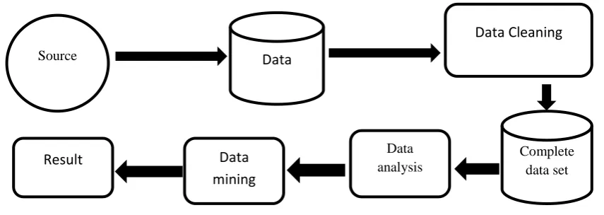
[image:1.595.77.505.382.534.2]

General Methodology

Fig. 1 Methodology

Fig 1 represents the methodology that we have used in this paper. Inthis, the data from the source is cleaned to obtain a complete dataset and then it is analysed using data mining techniques to obtain the required results. Each term in this methodology has been described below.

• Source:The source from which we can get the data. For example internet.

Revised Manuscript Received on March 08, 2019.

R.Subhashini, Professor, School of Computing, Sathyabama Institute of Science and Technology, Chennai, 600119, India.

J.K.Jeevitha, Assistant Professor, Department of Information Technology, PSNA College of Engineering and Technology, Dindigul.

B. KeerthiSamhitha, Assistant Professor, School of Computing, Sathyabama Institute of Science and Technology, Chennai, 600119, India.

• Data:The appropriate data set obtained from the source. • Data Cleaning: The data set obtained cannot be readily

used for analysis. This dataset should be pre-processedaccording to our use.

• Complete dataset:The dataset obtained may not be complete. There are several ways to handle the N/A value.

 Remove the rows that contain unknown values.  Find the similar cases referring other attributes and

fill the unknown value.

 Find the correlation or dependency of attributes and fill the unknown value,

Application of Data Mining Techniques to

Examine Quality of Water

R.Subhashini, J.K.Jeevitha, B. Keerthi Samhitha

Source

_Data

Data Cleaning

Data analysis

Result

Data

mining

(2)

 Find mean or median of the other available values of that particular attribute and fill the unknown value.

• Data analysis: The complete dataset obtained is to be analysed. We can even visualise the data using box plot, histogram, bar graph, simple plot etc..,

• Data mining: We have several data mining techniques such as clustering, classification, regression, decision trees, nearest neighbour method etc..,

• Result: The final predictions and analysis. Case Studies

Case Study 1

• Data: Algae dataset[3]

• Data description: This dataset consists of attributes such as maximum phvalue, minimum value of oxygen, mean value of chlorides, mean value of nitrates, mean value of ammonium, mean value of orthophosphate, mean value of phosphate, mean value of chlorophyll, frequencies of seven different algae.

• Correlation: In Eq 1 we can see that mean value of orthophosphate and phosphate are correlated.

PO4 = 42.897 + (1.293*OPO4) ……… Eq 1

• Using this we can fill the missing values of PO4 if we have the values of OPO4.

• Result: In this paper, we are going to prepare a model to predict the frequencies of seven different algae.

Case Study 2

The Chicago Park District keeps sensors in water at beaches beside Chicago’s Lake Michigan lakefront. These sensors generally capture the indicated measurements while sensors are in operation.

• Data: Beach water quality (automated sensors)[4] • Data description: This attributes in this dataset are water

temperature, turbidity, height of wave , period of wave, battery life and transducer’s depth and some other attributes such as name of beach, measurement time stamp, measurement id etc..,

• Cleaned data set: In this paper we will be considering only water temperature, turbidity, height of wave, period of wave, battery life and the transducer’s depth.

• Result: In this paper, we are going to prepare a model to predict the depth of the transducer.

II. METHOD

Multiple linear regression

It challenges to model association between two or moredescriptive variables and a response variable by anappropriatelinear equation to observed data .Every value of independent variable x is associated with dependant variable y.Eq 2 represents equation of a multiple linear regression.

Y=a0+a1x1+a2x2+a3x3+………aPxp ……….. Eq2

We can use lm () function to obtain this linear model. Result of this function is an object that contains all the information about this linear model.R will give us value and standard error of each coefficient of multiple linear regression equation. We can even test the importance of

estimate mean response or predict the future values of response variable .The function predict () can be used to make both confidence intervals for mean response and prediction intervals. We can partition the data set to use them as test and train data sets.

We can use nova() function to compare reduced and full models. This function even gives us a sequential analysis of variance of the model. Update() can be used to perform any small changes to the existing linear model.

Regression Trees

A regression tree is built through a process known as binary recursive partitioning which is an iterative process that splits data into partitions or branches and then continues splitting each partition into smaller groups. It consists of a single output and one or more input variables. This algorithm selects the splits that minimises the sum of squared deviations from the mean. This process continues until each node reaches a user specified minimum node size and becomes a terminal node.

We can use rpart() to generate this regression tree. This function uses the same schema as lm() to describe the functional form of the model. We can even specify the data to be used to generate the regression tree in its argument. As tree based models automatically selects more relevant variables, not all variables need to appear in the tree. At the leaf node we have the predictions of the tree. So if we want to use a tree to obtain a prediction for a particular water sample, we only need to follow a branch from root node until a leaf, according to the outcome of tests for that sample. We can use prettyTree () to visualise these results. We can prune the tree using prune () with respective cp value or else we can use rpartXse () which automates this process. We can use snip.rpart () for interactive pruning of a tree.

Random forest

Random forest (5) grows many classification trees. This technique uses averaging to find a natural balance between two extremes unlike the single decision trees which are likely to produce high variance. It can be used to naturally rank the importance of variables in a regression or classification.

In random forest there is no need of cross validation or a separate test set to get an unbiased estimate of test set error as it is estimated internally. The forest error rate mainly depends on correlation and strength.

Model evaluation and selection

Instead of using a single model to analyse and predict the whole data, we can make use of several such models and predict each data using an appropriate model.

(3)

We can use the mean absolute error or mean squared error or normalised mean squared error or any other standard error to compare these models.experimentalComparision ()

function can be used to compare and select an appropriate model.

III. RESULT

[image:3.595.83.512.116.383.2]

Case Study 1

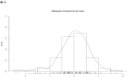
Fig. 2 Histogram of mxpH

[image:3.595.178.419.441.657.2]

Fig 2 is an enriched version of histogram of variable maximum pH. The curve represents the smooth version of histogram Using the jitter representation; we can easily find the outliers.

Fig. 3 Regression tree of algae data

(4)

Case Study 2

Fig. 4 (a) Plot of transducer’s depth predicted values against true values using linear model; (b) Plot of transducer’s depth predicted values against true values using regression tree

[image:4.595.69.530.80.287.2]

Fig 4 (a) represents the error scatter plot of linear model and Fig 4(b) represents the error scatter plot of regression model. Here the dotted line represents the equation y=x .If the points are close to this line, then the predicted values are close to real values.

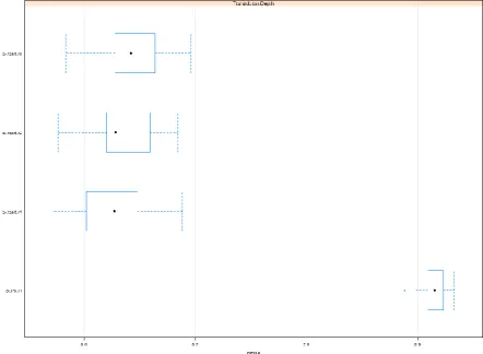
[image:4.595.71.514.365.689.2]

(5)

Fig 5 represents the box plots of various models. Here we can compare the NMSE values of various models. This can even be used to find the outliers. Using this plot, we can conclude that linear model is not appropriate to predict the transducer’s depth as error rate is high.

III. CONCLUSION

We have created a model through which we can predict the frequencies of seven different algae. If the numbers say that there is a chance of particular algal bloom then we can take preventive measures against those particular algae. Hence we can prevent the water from getting contaminated. By maintaining the quality of water, we can save aquatic, human and animal life. We can protect human from getting affected by serious diseases such as hepatitis, cholera, dengue etc.., and we can protect animals from getting affected because of food chain.We can protect the ecosystem. We can even save economic cost. Because it will cost a lot to purify contaminated water. Here we have considered only multiple linear regression, regression tree and random forest, but there are several other techniques which can be tried. Instead of using just algae, we can even use various such plants that contaminate water.

REFERENCES

1. Brian ALAN Whitton, Martyn Kelly (1995) Use of algae and other plants for monitoring rivers.

2. Tochukwu K. Anyachebelu, Marc Conrad, TahminaAjmal

(2014)Modelling and prediction of Surface Water Contamination using On-line Sensor Data.

3. Package ‘DMwR’ –CRAN

4. Beach Water Quality – Automated Sensors (2015)

http://catalog.data.gov/dataset/beach-water-quality-automated-sensors-66a4b