© 2005 Science Publications
Corresponding Author: M. Z. Yusoff, Department of Mechanical Engineering, Universiti Tenaga Nasional, Km. 7, Jalan Kajang-Puchong, 43009 Kajang, Selangor Darul Ehsan, Malaysia.
Simulations of Two-dimensional High Speed Turbulent Compressible Flow
in a Diffuser and a Nozzle Blade Cascade
K.C. Ng
, M.Z.Yusoff, T.F.Yusaf
Department of Mechanical Engineering, Universiti Tenaga Nasional,
Km. 7, Jalan Kajang-Puchong, 43009 Kajang, Selangor Darul Ehsan, Malaysia.
Abstract: This research describes the development of a new structured 2D CFD solver for compressible flow. The high-speed turbulent flow in a diffuser and a cascade of nozzle blade are predicted using standard k-
ε
turbulence model. The new finite volume CFD solver employs second-order accurate central differencing scheme for spatial discretization and multi-stage Runge-Kutta time integration to solve the set of non-linear governing equations with variables stored at the vertices. Artificial dissipations with pressure sensors are introduced to control solution stability and capture shock discontinuity. In general, the predictions compare well with the experimental measurements. Key words: CFD, compressible flow, cell-vertex, time-marching, turbulence modelINTRODUCTION
In general, there are two methods available in solving the compressible Navier-Stokes Equations (NSE). The most prominent method is to solve the system of non-linear equations in segregated manner by employing an iterative procedure in which solutions are alternately obtained for the pressure and velocity fields. The link is then provided by the continuity equation. In this algorithm, pressure is treated as the primary flow variable due to the fact that pressure gradient is always finite regardless of Mach regimes. Therefore, this is the common scheme employed by the modern commercial CFD codes due to the robustness of the numerical procedure. Known as Pressure Based Method (PBM), this algorithm has been applied extensively in incompressible flow field originally and has been extended to compressible flow by Issa and Lockwood[1], Van Doormaal et al.[2], McGuirk and Page[3], Watterson[4] and Jasak[5]. Notwithstanding this, due to the fact that the momentum, continuity and pressure equations are solved in an uncoupled approach, this may result in convergence problems, especially in situations where the gradients of flow variables are relatively large such as stagnation point at the leading edge. The idea of density variation in compressible flow field has led to the emergence of coupled solution technique since density exists as a dependent variable in the system of compressible Navier-Stokes equations. By realizing the capability of time-marching technique to circumvent the numerical difficulties in mixed subsonic-supersonic problem, time marching procedure has been utilized to solve the system of NSE in a coupled manner
by many researchers such as Denton[6], Ni[7], Dawes [8], Ollivier[9] and Lassaline[10].
The vast majority of fluid applications involve turbulence. Cases such as fluid flow in a pipe, flow processes in combustion chamber, flow over an airfoil will exhibit a chaotic complex motion defined as turbulent flow. While the popularity of Direct Numerical Simulation (DNS) and Large Eddy Simulation (LES) have become noticeable due to the rapid development of High-Performance Computing (HPC) technology, the general turbulent fluid motions are well described by the Reynolds-Averaged Navier-Stokes (RANS) equations with the inclusion of Reynolds stresses into the original full Navier-Stokes equation, which is computationally cheaper[8]. To resolve the Reynolds stresses, more equations are necessary and these extra equations are classified as turbulence models.
In this study, the new CFD solver will be used to investigate the high-speed compressible flow in a diffuser and nozzle blade cascade with standard k-
ε
turbulence model for closure. The idea presented is an extension of the original inviscid 2D solver for two-phase steam flow[11].MATHEMATICAL FORMULATION
W F G J
t x y
∂ ∂ ∂
∂ + ∂ +∂ = (1)
Where: 0 u v W e k ρ ρ ρ ρ ρ ρε = 2 0 1 ( ) ( ) xx xy x t k t u u P uv uh Q F k uk x u x ε ρ ρ τ ρ τ ρ µ ρ µ σ µ ε
ρ ε µ
σ
+ − −
+ − Φ
= ∂ − + ∂ ∂ − + ∂ 2 0 2 ( ) ( ) yx yy y t k t v uv v P vh Q G k vk y v y ε ρ ρ τ ρ τ ρ µ ρ µ σ µ ε
ρ ε µ
σ
− + −
+ − Φ
= ∂ − + ∂ ∂ − + ∂ 2 1 2 0 0 0 0 k k J P
C P C k k
ε ε
ρε
ε ρε
= −
−
W
is known as the conserved variables,F
andG
are the overall fluxes in x-, y- directions respectively andJ
represents the source vector.NUMERICAL SCHEMES
Solving Procedure: Starting from the flow field variables obtained from the previous time step, the conserved variables in RANS are solved with the appropriate boundary conditions. The updated variables are then substituted in the standard k-
ε
turbulence model to solve for turbulent kinetic energy and turbulent dissipation rate. Wall functions and turbulent boundary conditions are then imposed. The updated k andε
will be used to calculate the turbulent viscosity and the Reynolds stresses. Subsequently, the new Reynolds stresses will be utilized to solve RANS in the next iteration. The loop continues until convergence is achieved.Cell-vertex finite-volume spatial discretization: The flow domain is replaced by a finite number of grid points, which are generated algebraically by the built-in pre-processor[12]. The mesh system is commonly known as H-mesh and divides the physical domain into a set of discrete rectangular control volumes.
A cell-vertex formulation is used in which the flow variables are stored at four vertices of a quadrilateral cell. It has been shown by Martinelli[13], Dick[14], Swanson and Radiespiel[15] that cell-vertex formulation offers some advantages over the cell-centred one in which cell-vertex method offers higher accuracy on irregular grid. For a uniform mesh, there would be no difference between the cell-centred and cell-vertex schemes; however, cell-vertex scheme does not require extrapolation to the solid boundary to obtain the wall static pressure, which is necessary in solving the
momentum equations for cells adjacent to the solid boundary.
Starting from known values of primitive variables from the previous time-step, the values of
F
andG
are calculated for each node. Then the line integration is performed for each control volume in turn for the six conserved variables (RANS + k-ε
Turbulence Model). The discretized RANS:(2)
The discretized standard k-
ε
model: -(
)
1
ijTM ijTM ijTM TM ij
R = − F dy G− dx +J
Ω (3)
After the spatial integration, the cell residual will take the form:
( )
ij ij w R w t ∂∂ = (4)
where
R w
ij( )
represents the sum residuals from RANS or turbulence model.The calculated residuals apply to the values of properties within the cell, whereas, the variables are actually stored at the nodes. Consequently, they have to be redistributed to the four surrounding nodes. This is done by sharing the changes equally between the four nodes in the context of central differencing.
Thus, the equivalent discretized equation for a node will be:
( )
A A
w R w
t
∂
∂ = (5)
Artificial dissipations: All second-order central-differencing schemes, even with a stable time-step, suffer from certain tendencies to instability due to the odd-even decoupling near a discontinuity. The scheme can be stabilised by introducing a small amount of artificial viscosity, suggested by Jameson et al.[16]. First –order upwind differencing scheme may be used to remedy the stability problem, however, the scheme tends to damp the solution so much and alter the flow physics. Therefore, 2nd order accurate central differencing scheme, which is consistent to the framework of Navier-Stokes equations, is applied to both RANS and turbulence model in the
(
)
(
)
(
F dy G dx)
Jcurrent work with suitable amount of artificial viscosity.
This artificial viscosity formulation is a blend of second and fourth-order terms with a pressure switch to detect changes in pressure gradient[16]. After the addition of the dissipation terms, Equation (5) becomes:
( )
( )
A A
A
w
R w D w
t
∂
∂ = + (6)
The multi-stage runge-kutta time stepping: Equation (6) is integrated with respect to time by means of a four-stage Runge-Kutta time stepping scheme, as proposed by Jameson et al.[16]:
0 n,
w =w
(
)
1 0 0 0
1 ,
w =w + ∆
α
t R +D(
)
2 0 1 0
2 ,
w =w + ∆
α
t R +D(
)
3 0 2 0
3 ,
w =w + ∆α t R +D
(
)
4 0 3 0
4 ,
w =w + ∆
α
t R +D1 4
n
w + =w (7)
Where, the superscripts, n and n+1 refer to the time intervals in the main integration sequence, 1, 2, 3, 4 refer to the intermediate time-steps in the Runge-Kutta scheme. The coefficients
α α α α
1,
2,
3,
4are 0.250, 0.333, 0.500 and 1.000, respectively.Boundary conditions: The mathematical theory of incompletely parabolic PDEs indicates the number and type of boundary conditions for the unsteady compressible RANS. In the present work, Euler-type of boundary condition is applied except at solid wall where no-slip condition is imposed. At inlet, the total pressure, total temperature, flow angle, turbulent kinetic energy and turbulent dissipation rate are fixed, while the static pressure is extrapolated from the interior if the inflow is subsonic. Otherwise, all variables are fixed at inlet. At exit, if the outflow is subsonic, only the static pressure is fixed, while total pressure, total temperature and flow angle are extrapolated from the interior by zero-order extrapolation. If the exit flow is supersonic, all four variables are extrapolated from the interior. For k-
ε
transport equations, k andε
are extrapolated for arbitrary exit flow conditions.Periodic boundary condition is essential in simulating flow in turbomachines. The periodicity condition on the bounding streamlines is easily satisfied by treating the calculating points on each of the bounding streamline as if they are interior ones, by assuming that all properties are equal for corresponding points on each of the streamline. Nodes on the periodic
boundaries will have contributions from four corresponding cells on both sides of the boundaries.
On solid walls, the values for velocity components as well as k and
ε
are set to zero. Adiabatic condition is imposed. For nodes adjacent to the wall, wall functions are introduced to calculate k andε
.Initial conditions: To start the computation, initial flow field variables must be specified at all calculating points. In this approach, a linear variation of pressure between inlet and exit planes is assumed from which the pressures at all calculating points can be obtained. The tangency condition is enforced to obtain the velocity components at each calculating point and no variation of other properties along the pitch is assumed. Using the inlet stagnation temperature and pressure, the assumed static pressure and velocity components, other properties can be calculated using isentropic relations.
For turbulence models, k and
ε
are set to the values consistent to the inlet k andε
. The fluctuating Reynolds stresses are then calculated using Boussinesq relation.APPLICATIONS
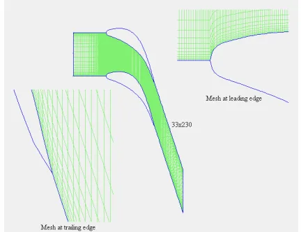
Blade-to-blade calculations on a turbine nozzle cascade: In order to validate the current solver, blade-to-blade flow simulation on a turbine nozzle blade cascade will be presented. The blade profile belongs to a stator of a low-pressure steam turbine. The geometry of the blade was generated using the in-house pre-processor of the current solver[12], as shown in Fig. 1. The experimental surface pressure measurements on the cascade were performed by Mamat[17].
Fig. 1: The blade geometry of the nozzle blade cascade
[image:3.612.319.535.486.653.2]corresponded to supersonic outlet, while 1.83 corresponded to transonic outlet. The flow conditions with subsonic outlet were represented by tests at an overall pressure ratio of 1.49.
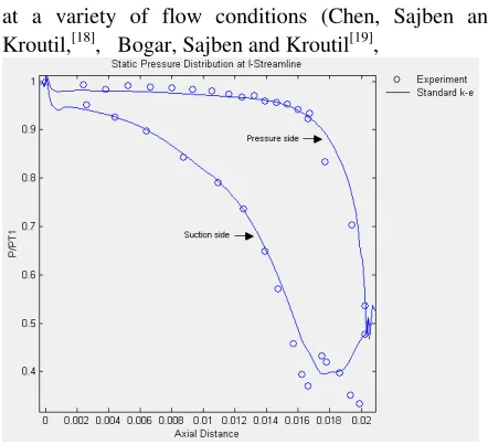
The mesh consisted of 33 x 230 grids. The mesh resolution near the wall was adjusted to be higher to account for the boundary layer development. A comparison of measured and calculated values of blade surface static pressure for subsonic flow, transonic flow and supersonic flow are illustrated in Fig. 2-4. In general, the numerical results show good agreement with the experimental data, except the pressure ratio at the trailing edge due to mesh distortion.
Fig. 2: Pressure plot at suction side for the nozzle cascade in subsonic flow condition
Fig. 3: Pressure plot at suction side for the nozzle cascade in transonic flow condition
Sajben diffuser: Transonic turbulent flow has been computed in a two-dimensional converging-diverging duct using the standard k- model. Extensive experimental data are available for this geometry,
at a variety of flow conditions (Chen, Sajben and Kroutil,[18], Bogar, Sajben and Kroutil[19],
[image:4.612.314.535.72.273.2]Fig. 4: Pressure plot at suction side for the nozzle cascade in supersonic flow condition
Fig. 5: The geometry of the sajben diffuser
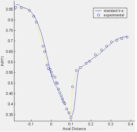
Fig. 6: Pressure plot at bottom wall for Pexit/Poinlet = 0.82 (weak shock)
[image:4.612.72.290.235.412.2] [image:4.612.70.290.235.635.2]Salmon, Bogar and Sajben[20], Sajben, Bogar and Kroutil[21],Bogar [22]). The flow fields being modelled were the weak- and strong-shock diffuser cases of Sajben[23]. The geometry of the diffuser is presented in Fig. 5.
[image:4.612.314.533.395.600.2] [image:4.612.71.288.456.633.2]pressure ratio (Pexit/Poinlet) was 0.82 and 0.72 for strong- and weak-shock case, respectively.
Figure 6 and 7 compares the pressure distributions along the bottom and top wall of the diffuser. The shock location predicted by the current solver compares well with the experimental data carried out at Pexit/Poinlet = 0.82 (weak shock). Next, the strong-shock case was simulated. Again, the illustrated results are comparable with the experimental data, except that the shock is predicted to occur 1 grid point further downstream as shown in Fig. 8 and 9. However, by considering the coarseness of the mesh employed in the current solver, the result is satisfactory.
Fig. 7: Pressure plot at top wall for Pexit/Poinlet = 0.82 (weak shock)
Fig. 8: Pressure plot at bottom wall for Pexit/Poinlet = 0.72 (strong shock)
Fig. 9: Pressure plot at top wall for Pexit/Poinlet = 0.72 (strong shock)
CONCLUSION
In the present work, a new two-dimensional compressible flow solver has been developed for structured grid. It uses the second-order accurate cell-vertex finite-volume spatial discretization and Runge-Kutta temporal integration. Standard k- turbulence model has been successfully adopted to simulate the compressible turbulent flow in a cascade of nozzle blade and Sajben diffuser. Both cases show good comparison with the experimental data, except the excessive smearing of shock wave at the trailing edge of the nozzle blade cascade. Research is still in progress on the existing turbulence model to compute the turbulent viscosity in a more accurate way.
Further work to be done on the solver includes the extension to 3D environment and modification to handle arbitrary meshes.
ACKNOWLEDGEMENT
This project is funded by the Ministry of Science Technology and Innovation (MOSTI), Malaysia under the IRPA Grant No. 09-99-03-0013-EA001 and UNITEN Internal Research Grant No. J510010026.
REFERENCES
[image:5.612.314.533.72.277.2] [image:5.612.72.290.236.445.2] [image:5.612.72.291.494.705.2]2. Van Doormaal, J.R., G.D. Raithby and B.H. McDonald, 1987. The segregated approach to predicting viscous compressible flow. J. Turbomachinery, Vol. 109.
3. McGuirk, J.J. and G.J. Page, 1990. Shock capturing using a pressure correction method. AIAA J., 28: 10.
4. Watterson, J.K., 1994. A pressure-based flow solver for the 3D navier stokes equation on unstructured and adaptive grids. 25th AIAA Fluid Dynamics Conf.
5. Jasak, H., 1996. Error analysis and estimation for the finite volume method with applications to fluid flow. Ph.D. Thesis, Imperial College.
6. Denton, J.D., 1975. A time marching method for two- and three-dimensional blade to blade flows. ARC R. & M. No. 3775.
7. Ni, R.H., 1982. A multiple grid scheme for solving the euler equations. AIAA J., 20: 1565-1571. 8. Dawes, W.N., 1991. The simulation of
three-dimensional viscous flow in turbomachinery geometries using a solution-adaptive unstructured mesh methodology. J. Turbomachinery, ASME 91-GT-124, Orlando.
9. Ollivier, C.F., 1995. Multigrid acceleration for an upwind euler solver on unstructured meshes. Preprint of AIAA J. Article.
10. Lassaline, J.V. and D.W. Zingg, 1998. Development of an agglomeration multigrid algorithm with directional coarsening. 14th AIAA Computational Fluid Dynamics.
11. Yusoff, M.Z., 1997. An improve treatmet of two-dimensional two-phase flows of steam by a runge-kutta method. Ph.D. Thesis, University of Birmingham.
12. Ng Khai Ching and Mohd. Zamri Yusoff, 2004. Report of UNITEN Research Project. Universiti Tenaga Nasional: Development on A User-Friendly 2D CFD Software For Teaching Fluid Dynamics: DYNAWORKS.
13. Martinelli, L., 1987. Calculations of viscous flows with a multigrid method. Ph.D. Thesis, MAE Department, Princeton University.
14. Dick, E., 1990. Introduction to Finite Volume Techniques, VKI Lecture Series.
15. Swanson, R.C. and R. Radespiel, 1991. Cell centered and cell vertex multigrid schemes for the navier stokes equations. AIAA J.
16. Jameson, A., W. Schmidt and E. Turkel, 1981. Numerical solutions of the euler equations by finite volume methods using runge-kutta time stepping schemes. AIAA Paper No. 81-1259.
17. Mamat, Z.A., 1996. The performance of a cascade of nozzle turbine blading in nucleating steam. Ph.D. Thesis, University of Birmingham.
18. Chen, C.P., M. Sajben and J.C. Kroutil, 1979. Shock wave oscillations in a transonic diffuser flow. AIAA J., 17: 1076-1083.
19. Bogar, T.J., M. Sajben and J.C. Kroutil, 1983. Characteristic frequencies of transonic diffuser flow oscillations. AIAA J., 21: 1232-1240.
20. Salmon, J.T., T.J. Bogar and M. Sajben, 1983. Laser doppler velocimeter measurements in unsteady, separated transonic diffuser flows. AIAA J., 21: 1690-1697.
21. Sajben, M., T.J. Bogar and J.C. Kroutil, 1984. Forced oscillation experiments in supercritical diffuser flows. AIAA J., 22: 465-474.
22. Bogar, T.J., 1986. Structure of self-excited oscillations in transonic diffuser flows. AIAA J., 24: 54-61.