Oracle Database
Oracle Database
11
g
SQL
Jason Price
New York Chicago San Francisco
Lisbon London Madrid Mexico City Milan
0-07-159613-5
The material in this eBook also appears in the print version of this title: 0-07-149850-8.
All trademarks are trademarks of their respective owners. Rather than put a trademark symbol after every occurrence of a trademarked name, we use names in an editorial fashion only, and to the benefit of the trademark owner, with no intention of infringement of the trademark. Where such designations appear in this book, they have been printed with initial caps.
McGraw-Hill eBooks are available at special quantity discounts to use as premiums and sales promotions, or for use in corporate training programs. For more information, please contact George Hoare, Special Sales, at [email protected] or (212) 904-4069.
TERMS OF USE
This is a copyrighted work and The McGraw-Hill Companies, Inc. (“McGraw-Hill”) and its licensors reserve all rights in and to the work. Use of this work is subject to these terms. Except as permitted under the Copyright Act of 1976 and the right to store and retrieve one copy of the work, you may not decompile, disassemble, reverse engineer, reproduce, modify, create derivative works based upon, transmit, distribute, disseminate, sell, publish or sublicense the work or any part of it without McGraw-Hill’s prior consent. You may use the work for your own noncommercial and personal use; any other use of the work is strictly prohibited. Your right to use the work may be terminated if you fail to comply with these terms.
We hope you enjoy this
McGraw-Hill eBook! If
you’d like more information about this book,
its author, or related books and websites,
please
click here.
Corporation. He has contributed to many of Oracle’s products, including the database, the application server, and several of the CRM applications. Jason is an Oracle Certified Database Administrator and Application Developer, and has more than 15 years of experience in the software industry. Jason has written many books on Oracle, Java, and .NET. Jason holds a Bachelor of Science degree (with honors) in physics from the University of Bristol, England.
About the Technical Editor
Contents at a Glance
1 Introduction . . . 1
2 Retrieving Information from Database Tables . . . 27
3 Using SQL*Plus . . . 63
4 Using Simple Functions . . . 89
5 Storing and Processing Dates and Times . . . 129
6 Subqueries . . . 167
7 Advanced Queries . . . 183
8 Changing Table Contents . . . 251
9 Users, Privileges, and Roles . . . 275
10 Creating Tables, Sequences, Indexes, and Views . . . 299
11 Introducing PL/SQL Programming . . . 339
12 Database Objects . . . 379
13 Collections . . . 427
14 Large Objects . . . 475
15 Running SQL Using Java . . . 531
16 SQL Tuning . . . 579
17 XML and the Oracle Database . . . 603
A Oracle Data Types . . . 635
Index . . . 639
Contents
Acknowledgments . . . xxiii
Introduction . . . xxv
1 Introduction . . . 1
What Is a Relational Database? . . . 2
Introducing the Structured Query Language (SQL) . . . 3
Using SQL*Plus . . . 4
Starting SQL*Plus . . . 4
Starting SQL*Plus from the Command Line . . . 6
Performing a SELECT Statement Using SQL*Plus . . . 6
SQL Developer . . . 7
Creating the Store Schema . . . 10
Running the SQL*Plus Script to Create the Store Schema . . . 10
Data Definition Language (DDL) Statements Used to Create the Store Schema . 11 Adding, Modifying, and Removing Rows . . . 20
Adding a Row to a Table . . . 20
Modifying an Existing Row in a Table . . . 22
Removing a Row from a Table . . . 22
The BINARY_FLOAT and BINARY_DOUBLE Types . . . 23
Benefits of BINARY_FLOAT and BINARY_DOUBLE . . . 23
Using BINARY_FLOAT and BINARY_DOUBLE in a Table . . . 24
Special Values . . . 24
Quitting SQL*Plus . . . 25
Introducing Oracle PL/SQL . . . 25
Summary . . . 26
2 Retrieving Information from Database Tables . . . 27
Performing Single Table SELECT Statements . . . 28
Retrieving All Columns from a Table . . . 29
Specifying Rows to Retrieve Using the WHERE Clause . . . 29
Row Identifiers . . . 30
Row Numbers . . . 30
Performing Arithmetic . . . 31
Performing Date Arithmetic . . . 31
Using Columns in Arithmetic . . . 32
Using Column Aliases . . . 34
Combining Column Output Using Concatenation . . . 35
Null Values . . . 35
Displaying Distinct Rows . . . 37
Comparing Values . . . 37
Using the SQL Operators . . . 39
Using the LIKE Operator . . . 40
Using the IN Operator . . . 41
Using the BETWEEN Operator . . . 42
Using the Logical Operators . . . 43
Operator Precedence . . . 44
Sorting Rows Using the ORDER BY Clause . . . 44
Performing SELECT Statements That Use Two Tables . . . 45
Using Table Aliases . . . 47
Cartesian Products . . . 48
Performing SELECT Statements That Use More than Two Tables . . . 49
Join Conditions and Join Types . . . 50
Non-equijoins . . . 50
Outer Joins . . . 51
Self Joins . . . 55
Performing Joins Using the SQL/92 Syntax . . . 56
Performing Inner Joins on Two Tables Using SQL/92 . . . 56
Simplifying Joins with the USING Keyword . . . 57
Performing Inner Joins on More than Two Tables Using SQL/92 . . . 58
Performing Inner Joins on Multiple Columns Using SQL/92 . . . 58
Performing Outer Joins Using SQL/92 . . . 59
Performing Self Joins Using SQL/92 . . . 60
Performing Cross Joins Using SQL/92 . . . 61
Summary . . . 61
3 Using SQL*Plus . . . 63
Viewing the Structure of a Table . . . 64
Editing SQL Statements . . . 65
Saving, Retrieving, and Running Files . . . 66
Formatting Columns . . . 70
Setting the Page Size . . . 72
Setting the Line Size . . . 73
Clearing Column Formatting . . . 73
Using Variables . . . 74
Temporary Variables . . . 74
Defined Variables . . . 77
Creating Simple Reports . . . 79
Using Temporary Variables in a Script . . . 80
Using Defined Variables in a Script . . . 80
Passing a Value to a Variable in a Script . . . 81
Adding a Header and Footer . . . 82
Getting Help from SQL*Plus . . . 85
Automatically Generating SQL Statements . . . 86
Disconnecting from the Database and Exiting SQL*Plus . . . 86
Summary . . . 87
4 Using Simple Functions . . . 89
Using Single-Row Functions . . . 90
Character Functions . . . 90
Numeric Functions . . . 98
Conversion Functions . . . 102
Regular Expression Functions . . . 109
Using Aggregate Functions . . . 117
AVG() . . . 118
COUNT() . . . 118
MAX() and MIN() . . . 119
STDDEV() . . . 120
SUM() . . . 120
VARIANCE() . . . 120
Grouping Rows . . . 120
Using the GROUP BY Clause to Group Rows . . . 121
Incorrect Usage of Aggregate Function Calls . . . 124
Using the HAVING Clause to Filter Groups of Rows . . . 125
Using the WHERE and GROUP BY Clauses Together . . . 126
Using the WHERE, GROUP BY, and HAVING Clauses Together . . . 126
Summary . . . 127
5 Storing and Processing Dates and Times . . . 129
Simple Examples of Storing and Retrieving Dates . . . 130
Converting Datetimes Using TO_CHAR() and TO_DATE() . . . 131
Using TO_CHAR() to Convert a Datetime to a String . . . 132
Using TO_DATE() to Convert a String to a Datetime . . . 136
Setting the Default Date Format . . . 139
How Oracle Interprets Two-Digit Years . . . 140
Using the YY Format . . . 140
Using the RR Format . . . 140
Using Datetime Functions . . . 142
ADD_MONTHS() . . . 142
LAST_DAY() . . . 144
MONTHS_BETWEEN() . . . 144
NEXT_DAY() . . . 144
ROUND() . . . 145
SYSDATE . . . 145
TRUNC() . . . 146
Using Time Zones . . . 146
Time Zone Functions . . . 147
The Database Time Zone and Session Time Zone . . . 147
Obtaining Time Zone Offsets . . . 149
Obtaining Time Zone Names . . . 149
Using Timestamps . . . 150
Using the Timestamp Types . . . 150
Timestamp Functions . . . 154
Using Time Intervals . . . 159
Using the INTERVAL YEAR TO MONTH Type . . . 160
Using the INTERVAL DAY TO SECOND Type . . . 162
Time Interval Functions . . . 164
Summary . . . 166
6 Subqueries . . . 167
Types of Subqueries . . . 168
Writing Single-Row Subqueries . . . 168
Subqueries in a WHERE Clause . . . 168
Using Other Single-Row Operators . . . 169
Subqueries in a HAVING Clause . . . 170
Subqueries in a FROM Clause (Inline Views) . . . 171
Errors You Might Encounter . . . 172
Writing Multiple-Row Subqueries . . . 173
Using IN with a Multiple-Row Subquery . . . 173
Using ANY with a Multiple-Row Subquery . . . 174
Using ALL with a Multiple-Row Subquery . . . 175
Writing Multiple-Column Subqueries . . . 175
Writing Correlated Subqueries . . . 175
A Correlated Subquery Example . . . 176
Using EXISTS and NOT EXISTS with a Correlated Subquery . . . 176
Writing Nested Subqueries . . . 179
Writing UPDATE and DELETE Statements Containing Subqueries . . . 180
Writing an UPDATE Statement Containing a Subquery . . . 180
Writing a DELETE Statement Containing a Subquery . . . 181
Summary . . . 181
7 Advanced Queries . . . 183
Using the Set Operators . . . 184
The Example Tables . . . 185
Using the UNION ALL Operator . . . 186
Using the UNION Operator . . . 187
Using the INTERSECT Operator . . . 188
Using the MINUS Operator . . . 188
Combining Set Operators . . . 188
Using the TRANSLATE() Function . . . 190
Using the DECODE() Function . . . 191
Using the CASE Expression . . . 193
Using Simple CASE Expressions . . . 193
Using Searched CASE Expressions . . . 194
Hierarchical Queries . . . 196
The Example Data . . . 196
Using the CONNECT BY and START WITH Clauses . . . 198
Using the LEVEL Pseudo Column . . . 198
Formatting the Results from a Hierarchical Query . . . 199
Starting at a Node Other than the Root . . . 200
Traversing Upward Through the Tree . . . 201
Eliminating Nodes and Branches from a Hierarchical Query . . . 201
Including Other Conditions in a Hierarchical Query . . . 202
Using the Extended GROUP BY Clauses . . . 203
The Example Tables . . . 203
Using the ROLLUP Clause . . . 205
Using the CUBE Clause . . . 207
Using the GROUPING() Function . . . 209
Using the GROUPING SETS Clause . . . 211
Using the GROUPING_ID() Function . . . 212
Using a Column Multiple Times in a GROUP BY Clause . . . 214
Using the GROUP_ID() Function . . . 215
Using the Analytic Functions . . . 216
The Example Table . . . 216
Using the Ranking Functions . . . 217
Using the Inverse Percentile Functions . . . 224
Using the Window Functions . . . 225
Using the Reporting Functions . . . 230
Using the LAG() and LEAD() Functions . . . 232
Using the FIRST and LAST Functions . . . 233
Using the Linear Regression Functions . . . 233
Using the Hypothetical Rank and Distribution Functions . . . 235
Using the MODEL Clause . . . 236
An Example of the MODEL Clause . . . 236
Using Positional and Symbolic Notation to Access Cells . . . 237
Accessing a Range of Cells Using BETWEEN and AND . . . 238
Accessing All Cells Using ANY and IS ANY . . . 238
Getting the Current Value of a Dimension Using CURRENTV() . . . 239
Accessing Cells Using a FOR Loop . . . 240
Handling Null and Missing Values . . . 241
Updating Existing Cells . . . 243
Using the PIVOT and UNPIVOT Clauses . . . 244
A Simple Example of the PIVOT Clause . . . 244
Pivoting on Multiple Columns . . . 246
Using Multiple Aggregate Functions in a Pivot . . . 247
Using the UNPIVOT Clause . . . 248
Summary . . . 249
8 Changing Table Contents . . . 251
Adding Rows Using the INSERT Statement . . . 252
Omitting the Column List . . . 253
Specifying a Null Value for a Column . . . 253
Including Single and Double Quotes in a Column Value . . . 254
Copying Rows from One Table to Another . . . 254
Modifying Rows Using the UPDATE Statement . . . 254
The RETURNING Clause . . . 255
Removing Rows Using the DELETE Statement . . . 256
Database Integrity . . . 256
Enforcement of Primary Key Constraints . . . 257
Using Default Values . . . 258
Merging Rows Using MERGE . . . 259
Database Transactions . . . 262
Committing and Rolling Back a Transaction . . . 262
Starting and Ending a Transaction . . . 263
Savepoints . . . 264
ACID Transaction Properties . . . 265
Concurrent Transactions . . . 266
Transaction Locking . . . 266
Transaction Isolation Levels . . . 267
A SERIALIZABLE Transaction Example . . . 269
Query Flashbacks . . . 270
Granting the Privilege for Using Flashbacks . . . 270
Time Query Flashbacks . . . 270
System Change Number Query Flashbacks . . . 272
Summary . . . 273
9 Users, Privileges, and Roles . . . 275
Users . . . 276
Creating a User . . . 276
Changing a User’s Password . . . 277
Deleting a User . . . 278
System Privileges . . . 278
Granting System Privileges to a User . . . 278
Checking System Privileges Granted to a User . . . 280
Making Use of System Privileges . . . 281
Revoking System Privileges from a User . . . 281
Object Privileges . . . 281
Granting Object Privileges to a User . . . 282
Checking Object Privileges Made . . . 283
Checking Object Privileges Received . . . 284
Making Use of Object Privileges . . . 286
Synonyms . . . 287
Public Synonyms . . . 287
Revoking Object Privileges . . . 288
Roles . . . 289
Creating Roles . . . 289
Granting Privileges to Roles . . . 290
Granting Roles to a User . . . 290
Checking Roles Granted to a User . . . 290
Checking System Privileges Granted to a Role . . . 291
Checking Object Privileges Granted to a Role . . . 292
Making Use of Privileges Granted to a Role . . . 293
Default Roles . . . 294
Revoking a Role . . . 294
Revoking Privileges from a Role . . . 294
Dropping a Role . . . 295
Auditing . . . 295
Privileges Required to Perform Auditing . . . 295
Audit Trail Views . . . 297
Summary . . . 297
10 Creating Tables, Sequences, Indexes, and Views . . . 299
Tables . . . 300
Creating a Table . . . 300
Getting Information on Tables . . . 302
Getting Information on Columns in Tables . . . 303
Altering a Table . . . 303
Renaming a Table . . . 313
Adding a Comment to a Table . . . 313
Truncating a Table . . . 314
Dropping a Table . . . 314
Sequences . . . 314
Creating a Sequence . . . 314
Retrieving Information on Sequences . . . 316
Using a Sequence . . . 317
Populating a Primary Key Using a Sequence . . . 319
Modifying a Sequence . . . 320
Dropping a Sequence . . . 320
Indexes . . . 320
Creating a B-tree Index . . . 321
Creating a Function-Based Index . . . 322
Retrieving Information on Indexes . . . 323
Retrieving Information on the Indexes on a Column . . . 323
Modifying an Index . . . 324
Dropping an Index . . . 324
Creating a Bitmap Index . . . 324
Views . . . 325
Creating and Using a View . . . 326
Modifying a View . . . 333
Dropping a View . . . 334
Flashback Data Archives . . . 334
Summary . . . 337
11 Introducing PL/SQL Programming . . . 339
Block Structure . . . 340
Variables and Types . . . 342
Conditional Logic . . . 342
Loops . . . 343
Simple Loops . . . 343
WHILE Loops . . . 344
FOR Loops . . . 344
Cursors . . . 345
Step 1: Declare the Variables to Store the Column Values . . . 346
Step 2: Declare the Cursor . . . 346
Step 3: Open the Cursor . . . 346
Step 4: Fetch the Rows from the Cursor . . . 347
Step 5: Close the Cursor . . . 347
Cursors and FOR Loops . . . 349
OPEN-FOR Statement . . . 350
Unconstrained Cursors . . . 352
Exceptions . . . 353
ZERO_DIVIDE Exception . . . 355
DUP_VAL_ON_INDEX Exception . . . 356
INVALID_NUMBER Exception . . . 356
OTHERS Exception . . . 357
Procedures . . . 358
Creating a Procedure . . . 358
Calling a Procedure . . . 360
Getting Information on Procedures . . . 361
Dropping a Procedure . . . 362
Viewing Errors in a Procedure . . . 362
Functions . . . 363
Creating a Function . . . 363
Calling a Function . . . 364
Getting Information on Functions . . . 365
Dropping a Function . . . 365
Packages . . . 365
Creating a Package Specification . . . 365
Creating a Package Body . . . 366
Calling Functions and Procedures in a Package . . . 367
Getting Information on Functions and Procedures in a Package . . . 368
Dropping a Package . . . 368
Triggers . . . 369
When a Trigger Fires . . . 369
Set Up for the Example Trigger . . . 369
Creating a Trigger . . . 369
Firing a Trigger . . . 371
Getting Information on Triggers . . . 372
Disabling and Enabling a Trigger . . . 374
Dropping a Trigger . . . 374
New Oracle Database 11g PL/SQL Features . . . 374
SIMPLE_INTEGER Type . . . 375
Sequences in PL/SQL . . . 375
PL/SQL Native Machine Code Generation . . . 377
Summary . . . 377
12 Database Objects . . . 379
Introducing Objects . . . 380
Creating Object Types . . . 381
Using DESCRIBE to Get Information on Object Types . . . 382
Using Object Types in Database Tables . . . 383
Column Objects . . . 383
Object Tables . . . 386
Object Identifiers and Object References . . . 390
Comparing Object Values . . . 392
Using Objects in PL/SQL . . . 394
The get_products() Function . . . 395
The insert_product() Procedure . . . 397
The update_product_price() Procedure . . . 398
The get_product() Function . . . 398
The update_product() Procedure . . . 399
The get_product_ref() Function . . . 400
The delete_product() Procedure . . . 400
The product_lifecycle() Procedure . . . 401
The product_lifecycle2() Procedure . . . 402
Type Inheritance . . . 403
Using a Subtype Object in Place of a Supertype Object . . . 405
SQL Examples . . . 405
PL/SQL Examples . . . 406
NOT SUBSTITUTABLE Objects . . . 407
Other Useful Object Functions . . . 408
IS OF() . . . 408
TREAT() . . . 412
SYS_TYPEID() . . . 416
NOT INSTANTIABLE Object Types . . . 416
User-Defined Constructors . . . 418
Overriding Methods . . . 422
Generalized Invocation . . . 423
Summary . . . 425
13 Collections . . . 427
Introducing Collections . . . 428
Creating Collection Types . . . 429
Creating a Varray Type . . . 429
Creating a Nested Table Type . . . 429
Using a Collection Type to Define a Column in a Table . . . 430
Using a Varray Type to Define a Column in a Table . . . 430
Using a Nested Table Type to Define a Column in a Table . . . 430
Getting Information on Collections . . . 431
Getting Information on a Varray . . . 431
Getting Information on a Nested Table . . . 432
Populating a Collection with Elements . . . 434
Populating a Varray with Elements . . . 434
Populating a Nested Table with Elements . . . 434
Retrieving Elements from Collections . . . 435
Retrieving Elements from a Varray . . . 435
Retrieving Elements from a Nested Table . . . 436
Using TABLE() to Treat a Collection as a Series of Rows . . . 436
Using TABLE() with a Varray . . . 437
Using TABLE() with a Nested Table . . . 438
Modifying Elements of Collections . . . 438
Modifying Elements of a Varray . . . 438
Modifying Elements of a Nested Table . . . 439
Using a Map Method to Compare the Contents of Nested Tables . . . 440
Using CAST() to Convert Collections from One Type to Another . . . 443
Using CAST() to Convert a Varray to a Nested Table . . . 443
Using Collections in PL/SQL . . . 444
Manipulating a Varray . . . 444
Manipulating a Nested Table . . . 446
PL/SQL Collection Methods . . . 448
Multilevel Collections . . . 458
Oracle Database 10g Enhancements to Collections . . . 461
Associative Arrays . . . 462
Changing the Size of an Element Type . . . 463
Increasing the Number of Elements in a Varray . . . 463
Using Varrays in Temporary Tables . . . 463
Using a Different Tablespace for a Nested Table’s Storage Table . . . 463
ANSI Support for Nested Tables . . . 464
Summary . . . 473
14 Large Objects . . . 475
Introducing Large Objects (LOBs) . . . 476
The Example Files . . . 476
Large Object Types . . . 477
Creating Tables Containing Large Objects . . . 478
Using Large Objects in SQL . . . 478
Using CLOBs and BLOBs . . . 478
Using BFILEs . . . 481
Using Large Objects in PL/SQL . . . 482
APPEND() . . . 485
CLOSE() . . . 485
COMPARE() . . . 486
COPY() . . . 487
CREATETEMPORARY() . . . 488
ERASE() . . . 488
FILECLOSE() . . . 489
FILECLOSEALL() . . . 489
FILEEXISTS() . . . 490
FILEGETNAME() . . . 490
FILEISOPEN() . . . 490
FILEOPEN() . . . 491
FREETEMPORARY() . . . 492
GETCHUNKSIZE() . . . 492
GET_STORAGE_LIMIT() . . . 492
GETLENGTH() . . . 493
INSTR() . . . 493
ISOPEN() . . . 494
ISTEMPORARY() . . . 495
LOADFROMFILE() . . . 496
LOADBLOBFROMFILE() . . . 497
LOADCLOBFROMFILE() . . . 497
OPEN() . . . 498
READ() . . . 499
SUBSTR() . . . 500
WRITE() . . . 502
WRITEAPPEND() . . . 503
Example PL/SQL Procedures . . . 503
LONG and LONG RAW Types . . . 521
The Example Tables . . . 521
Adding Data to LONG and LONG RAW Columns . . . 521
Converting LONG and LONG RAW Columns to LOBs . . . 522
Oracle Database 10g Enhancements to Large Objects . . . 523
Implicit Conversion Between CLOB and NCLOB Objects . . . 523
Use of the :new Attribute When Using LOBs in a Trigger . . . 524
Oracle Database 11g Enhancements to Large Objects . . . 525
Encrypting LOB Data . . . 525
Compressing LOB Data . . . 529
Removing Duplicate LOB Data . . . 529
Summary . . . 529
15 Running SQL Using Java . . . 531
Getting Started . . . 532
Configuring Your Computer . . . 533
Setting the ORACLE_HOME Environment Variable . . . 533
Setting the JAVA_HOME Environment Variable . . . 534
Setting the PATH Environment Variable . . . 534
Setting the CLASSPATH Environment Variable . . . 534
Setting the LD_LIBRARY_PATH Environment Variable . . . 535
The Oracle JDBC Drivers . . . 535
The Thin Driver . . . 535
The OCI Driver . . . 536
The Server-Side Internal Driver . . . 536
The Server-Side Thin Driver . . . 536
Importing the JDBC Packages . . . 536
Registering the Oracle JDBC Drivers . . . 537
Opening a Database Connection . . . 537
Connecting to the Database Using getConnection() . . . 537
The Database URL . . . 538
Connecting to the Database Using an Oracle Data Source . . . 539
Creating a JDBC Statement Object . . . 542
Retrieving Rows from the Database . . . 543
Step 1: Create and Populate a ResultSet Object . . . 543
Step 2: Read the Column Values from the ResultSet Object . . . 544
Step 3: Close the ResultSet Object . . . 546
Adding Rows to the Database . . . 547
Modifying Rows in the Database . . . 548
Deleting Rows from the Database . . . 548
Handling Numbers . . . 549
Handling Database Null Values . . . 550
Controlling Database Transactions . . . 552
Performing Data Definition Language Statements . . . 553
Handling Exceptions . . . 553
Example Program: BasicExample1.java . . . 556 Compile BasicExample1 . . . 560 Run BasicExample1 . . . 561 Prepared SQL Statements . . . 562 Example Program: BasicExample2.java . . . 565 The Oracle JDBC Extensions . . . 567 The oracle.sql Package . . . 568 The oracle.jdbc Package . . . 571 Example Program: BasicExample3.java . . . 575 Summary . . . 578
16 SQL Tuning . . . 579
Introducing SQL Tuning . . . 580 Use a WHERE Clause to Filter Rows . . . 580 Use Table Joins Rather than Multiple Queries . . . 581 Use Fully Qualified Column References When Performing Joins . . . 582 Use CASE Expressions Rather than Multiple Queries . . . 583 Add Indexes to Tables . . . 584 Use WHERE Rather than HAVING . . . 584 Use UNION ALL Rather than UNION . . . 585 Use EXISTS Rather than IN . . . 586 Use EXISTS Rather than DISTINCT . . . 587 Use GROUPING SETS Rather than CUBE . . . 588 Use Bind Variables . . . 588 Non-Identical SQL Statements . . . 588 Identical SQL Statements That Use Bind Variables . . . 588 Listing and Printing Bind Variables . . . 590 Using a Bind Variable to Store a Value Returned by a PL/SQL Function . . . 590 Using a Bind Variable to Store Rows from a REFCURSOR . . . 590 Comparing the Cost of Performing Queries . . . 591 Examining Execution Plans . . . 591 Comparing Execution Plans . . . 597 Passing Hints to the Optimizer . . . 598 Additional Tuning Tools . . . 600 Oracle Enterprise Manager Diagnostics Pack . . . 600 Automatic Database Diagnostic Monitor . . . 600 Summary . . . 601
17 XML and the Oracle Database . . . 603
XMLSEQUENCE() . . . 615 XMLSERIALIZE() . . . 616 A PL/SQL Example That Writes XML Data to a File . . . 616 XMLQUERY() . . . 618 Saving XML in the Database . . . 622 The Example XML File . . . 623 Creating the Example XML Schema . . . 623 Retrieving Information from the Example XML Schema . . . 625 Updating Information in the Example XML Schema . . . 630 Summary . . . 633
A Oracle Data Types . . . 635
Oracle SQL Types . . . 636 Oracle PL/SQL Types . . . 638
Acknowledgments
hanks to the wonderful people at McGraw-Hill, including Lisa McClain, Mandy Canales, Carl Wikander, and Laura Stone. Thanks also to Scott Mikolaitis for his thorough technical review.
T
Introduction
oday’s database management systems are accessed using a standard language known as Structured Query Language, or SQL. Among other things, SQL allows you to retrieve, add, update, and delete information in a database. In this book, you’ll learn how to master SQL, and you’ll find a wealth of practical examples. You can also get all the scripts and programs featured in this book online (see the last section, “Retrieving the Examples,” for details).
With this book, you will
Master standard SQL, as well as the extensions developed by Oracle Corporation for use with the specific features of the Oracle database.
Explore PL/SQL (Procedural Language/SQL), which is built on top of SQL and enables you to write programs that contain SQL statements.
Use SQL*Plus to execute SQL statements, scripts, and reports; SQL*Plus is a tool that allows you to interact with the database.
Execute queries, inserts, updates, and deletes against a database. Create database tables, sequences, indexes, views, and users. Perform transactions containing multiple SQL statements.
Define database object types and create object tables to handle advanced data. Use large objects to handle multimedia files containing images, music, and movies. Perform complex calculations using analytic functions.
Use all the very latest Oracle Database 11gfeatures such asPIVOTandUNPIVOT, flashback archives, and much more.
Implement high-performance tuning techniques to make your SQL statements really fly.
■
■
■
■ ■ ■ ■ ■ ■ ■
■
T
Write Java programs to access an Oracle database using JDBC. Explore the XML capabilities of the Oracle database.
This book contains 17 chapters and one appendix.
Chapter 1: Introduction
In this chapter, you’ll learn about relational databases, be introduced to SQL, see a few simple queries, use SQL*Plus and SQL Developer to execute queries, and briefly see PL/SQL.
Chapter 2: Retrieving Information from Database Tables
You’ll explore how to retrieve information from one or more database tables using SELECT
statements, use arithmetic expressions to perform calculations, filter rows using a WHERE clause, and sort the rows retrieved from a table.
Chapter 3: Using SQL*Plus
In this chapter, you’ll use SQL*Plus to view a table’s structure, edit a SQL statement, save and run scripts, format column output, define and use variables, and create reports.
Chapter 4: Using Simple Functions
In this chapter, you’ll learn about some of the Oracle database’s built-in functions. A function can accept input parameters and returns an output parameter. Functions allow you to perform tasks such as computing averages and square roots of numbers.
Chapter 5: Storing and Processing Dates and Times
You’ll learn how the Oracle database processes and stores dates and times, collectively known as datetimes. You’ll also learn about timestamps that allow you to store a specific date and time, and time intervals that allow you to store a length of time.
Chapter 6: Subqueries
You’ll learn how to place a SELECT statement within an outer SQL statement. The inner SELECT
statement is known as a subquery. You’ll learn about the different types of subqueries and see how subqueries allow you to build up very complex statements from simple components.
Chapter 7: Advanced Queries
In this chapter, you’ll learn how to perform queries containing advanced operators and functions such as: set operators that combine rows returned by multiple queries, the TRANSLATE()
function to convert characters in one string to characters in another string, the DECODE() function to search a set of values for a certain value, the CASE expression to perform if-then-else logic, and the ROLLUP and CUBE clauses to return rows containing subtotals. You’ll learn about the analytic functions that enable you to perform complex calculations such as finding the top-selling product type for each month, the top salespersons, and so on. You’ll see how to perform queries against data that is organized into a hierarchy. You’ll also explore the MODEL clause, which performs inter-row calculations. Finally, you’ll see the new Oracle Database 11gPIVOT and UNPIVOT
clauses, which are useful for seeing overall trends in large amounts of data.
Chapter 8: Changing Table Contents
You’ll learn how to add, modify, and remove rows using the INSERT, UPDATE, and DELETE
statements, and how to make the results of your transactions permanent using the COMMIT
statement or undo their results entirely using the ROLLBACK statement. You’ll also learn how an Oracle database can process multiple transactions at the same time.
Chapter 9: Users, Privileges, and Roles
In this chapter, you’ll learn about database users and see how privileges and roles are used to enable users to perform specific tasks in the database.
Chapter 10: Creating Tables, Sequences, Indexes, and Views
You’ll learn about tables and sequences, which generate a series of numbers, and indexes, which act like an index in a book and allow you quick access to rows. You’ll also learn about views, which are predefined queries on one or more tables; among other benefits, views allow you to hide complexity from a user, and implement another layer of security by only allowing a view to access a limited set of data in the tables. You’ll also examine flashback data archives, which are new for Oracle Database 11g. A flashback data archive stores changes made to a table over a period of time.
Chapter 11: Introducing PL/SQL Programming
In this chapter, you’ll explore PL/SQL, which is built on top of SQL and enables you to write stored programs in the database that contain SQL statements. PL/SQL contains standard programming constructs.
Chapter 12: Database Objects
You’ll learn how to create database object types, which may contain attributes and methods. You’ll use object types to define column objects and object tables, and see how to manipulate objects using SQL and PL/SQL.
Chapter 13: Collections
In this chapter, you’ll learn how to create collection types, which may contain multiple elements. You’ll use collection types to define columns in tables. You’ll see how to manipulate collections using SQL and PL/SQL.
Chapter 14: Large Objects
You’ll learn about large objects, which can be used to store up to 128 terabytes of character and binary data or point to an external file. You’ll also learn about the older LONG types, which are still supported in Oracle Database 11g for backward compatibility.
Chapter 15: Running SQL Using Java
Chapter 16: SQL Tuning
You’ll see SQL tuning tips that you can use to shorten the length of time your queries take to execute. You’ll also learn about the Oracle optimizer and examine how to pass hints to the optimizer.
Chapter 17: XML and the Oracle Database
The Extensible Markup Language (XML) is a general-purpose markup language. XML enables you to share structured data across the Internet, and can be used to encode data and other documents. In this chapter, you’ll see how to generate XML from relational data and how to save XML in the database.
Appendix: Oracle Data Types
This appendix shows the data types available in Oracle SQL and PL/SQL.
Intended Audience
This book is suitable for the following readers:
Developers who need to write SQL and PL/SQL.
Database administrators who need in-depth knowledge of SQL.
Business users who need to write SQL queries to get information from their organization’s database.
Technical managers or consultants who need an introduction to SQL and PL/SQL. No prior knowledge of the Oracle database, SQL, or PL/SQL is assumed; you can find everything you need to know to become a master in this book.
Retrieving the Examples
All the SQL scripts, programs, and other files used in this book can be downloaded from the Oracle Press website at www.OraclePressBooks.com. The files are contained in a Zip file. Once you’ve downloaded the Zip file, you need to extract its contents. This will create a directory named sql_book that contains the following subdirectories:
Java Contains the Java programs used in Chapter 15
sample_files Contains the sample files used in Chapter 14
SQL Contains the SQL scripts used throughout the book, including scripts to create and populate the example database tables
xml_files Contains the XML used in Chapter 17 I hope you enjoy this book!
■ ■ ■
■
■ ■ ■
CHAPTER
1
Introduction
n this chapter, you will learn about the following:
I
Relational databases.The Structured Query Language (SQL), which is used to access a database. SQL*Plus, Oracle’s interactive text-based tool for running SQL statements. SQL Developer, which is a graphical tool for database development. PL/SQL, Oracle’s procedural programming language. PL/SQL allows you to develop programs that are stored in the database.
■ ■ ■ ■ ■
Let’s plunge in and consider what a relational database is.
What Is a Relational Database?
The concept of a relational database was originally developed back in 1970 by Dr. E.F. Codd. He laid down the theory of relational databases in his seminal paper entitled “A Relational Model of Data for Large Shared Data Banks,” published in Communications of the ACM (Association for Computing Machinery), Vol. 13, No. 6, June 1970.
The basic concepts of a relational database are fairly easy to understand. A relational database
is a collection of related information that has been organized into tables. Each table stores data in
rows; the data is arranged into columns. The tables are stored in database schemas, which are areas where users may store their own tables. A user may grant permissions to other users so they can access their tables.
Most of us are familiar with data being stored in tables—stock prices and train timetables are sometimes organized into tables. One example table used in this book records customer information for an imaginary store; the table stores the customer first names, last names, dates of birth (dobs), and phone numbers:
first_name last_name dob phone
--- --- --- ---John Brown 01-JAN-1965 800-555-1211 Cynthia Green 05-FEB-1968 800-555-1212 Steve White 16-MAR-1971 800-555-1213 Gail Black 800-555-1214 Doreen Blue 20-MAY-1970
This table could be stored in a variety of forms: A card in a box
An HTML file on a web page A table in a database
An important point to remember is that the information that makes up a database is different from the system used to access that information. The software used to access a database is known as a database management system. The Oracle database is one such piece of software; other examples include SQL Server, DB2, and MySQL.
Of course, every database must have some way to get data in and out of it, preferably using a common language understood by all databases. Database management systems implement a standard language known as Structured Query Language, or SQL. Among other things, SQL allows you to retrieve, add, modify, and delete information in a database.
Introducing the Structured Query Language (SQL)
Structured Query Language (SQL) is the standard language designed to access relational databases. SQL should be pronounced as the letters “S-Q-L.”
NOTE
“S-Q-L” is the correct way to pronounce SQL according to the American National Standards Institute. However, the single word “sequel” is frequently used instead.
SQL is based on the groundbreaking work of Dr. E.F. Codd, with the first implementation of SQL being developed by IBM in the mid-1970s. IBM was conducting a research project known as System R, and SQL was born from that project. Later, in 1979, a company then known as Relational Software Inc. (known today as Oracle Corporation) released the first commercial version of SQL. SQL is now fully standardized and recognized by the American National Standards Institute.
SQL uses a simple syntax that is easy to learn and use. You’ll see some simple examples of its use in this chapter. There are five types of SQL statements, outlined in the following list:
Query statements retrieve rows stored in database tables. You write a query using the SQL SELECT statement.
Data Manipulation Language (DML) statements modify the contents of tables. There are three DML statements:
INSERT adds rows to a table.
UPDATE changes rows.
DELETE removes rows.
Data Definition Language (DDL) statements define the data structures, such as tables, that make up a database. There are five basic types of DDL statements:
CREATE creates a database structure. For example, CREATE TABLE is used to create a table; another example is CREATE USER, which is used to create a database user.
ALTER modifies a database structure. For example, ALTER TABLE is used to modify a table.
DROP removes a database structure. For example, DROP TABLE is used to remove a table.
RENAME changes the name of a table.
TRUNCATE deletes all the rows from a table.
■
■
■ ■ ■ ■
■
■
■
Transaction Control (TC) statements either permanently record any changes made to rows, or undo those changes. There are three TC statements:
COMMIT permanently records changes made to rows.
ROLLBACK undoes changes made to rows.
SAVEPOINT sets a “save point” to which you can roll back changes.
Data Control Language (DCL) statements change the permissions on database structures. There are two DCL statements:
GRANT gives another user access to your database structures.
REVOKE prevents another user from accessing your database structures.
There are many ways to run SQL statements and get results back from the database, some of which include programs written using Oracle Forms and Reports. SQL statements may also be embedded within programs written in other languages, such as Oracle’s Pro*C++, which allows you to add SQL statements to a C++ program. You can also add SQL statements to a Java program using JDBC; for more details, see my book Oracle9i JDBC Programming (Oracle Press, 2002).
Oracle also has a tool called SQL*Plus that allows you to enter SQL statements using the keyboard or to run a script containing SQL statements. SQL*Plus enables you to conduct a “conversation” with the database; you enter SQL statements and view the results returned by the database. You’ll be introduced to SQL*Plus next.
Using SQL*Plus
If you’re at all familiar with the Oracle database, chances are that you’re already familiar with SQL*Plus. If you’re not, don’t worry: you’ll learn how to use SQL*Plus in this book.
In the following sections, you’ll learn how to start SQL*Plus and run a query.
Starting SQL*Plus
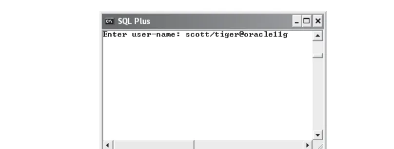
If you’re using Windows XP Professional Edition and Oracle Database 11g, you can start SQL*Plus by clicking start and selecting All Programs | Oracle | Application Development | SQL Plus.
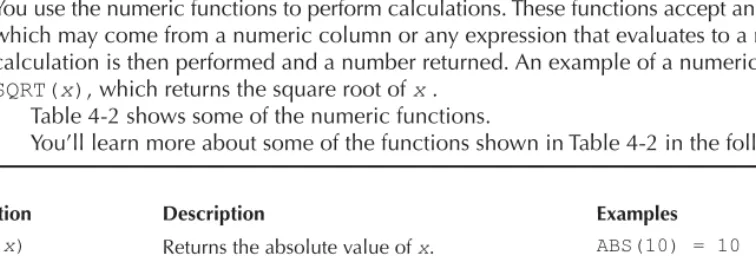
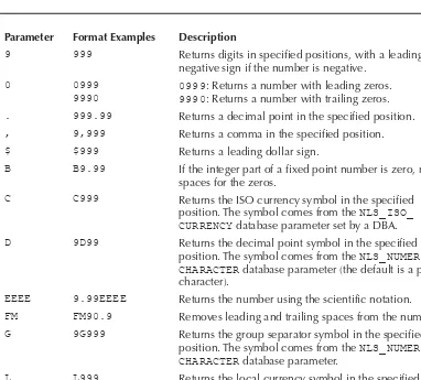
Figure 1-1 shows SQL*Plus running on Windows XP. SQL*Plus asks you for a username. Figure 1-1 shows the scott user connecting to the database (scott is an example user that is contained in many Oracle databases; scott has a default password of tiger). The host string after the @ character tells SQL*Plus where the database is running. If you are running the database on your own computer, you’ll typically omit the host string (that is, you enter scott/ tiger)—doing this causes SQL*Plus to attempt to connect to a database on the same machine on which SQL*Plus is running. If the database isn’t running on your machine, you should speak with your database administrator (DBA) to get the host string. If the scott user doesn’t exist or is locked, ask your DBA for an alternative user and password (for the examples in the first part of this chapter, you can use any user; you don’t absolutely have to use the scott user).
■
■ ■ ■ ■
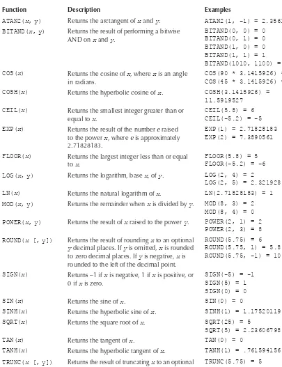
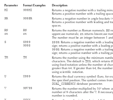
If you’re using Windows XP and Oracle Database 10g or below, you can run a special Windows-only version of SQL*Plus. You start this version of SQL*Plus by clicking Start and selecting All Programs | Oracle | Application Development | SQL Plus. The Windows-only version of SQL*Plus is deprecated in Oracle Database 11g (that is, it doesn’t ship with 11g),
but it will still connect to an 11g database. Figure 1-2 shows the Windows-only version of Oracle Database 10g SQL*Plus running on Windows XP.
NOTE
The Oracle Database 11g version of SQL*Plus is slightly nicer than the Windows-only version. In the 11g version, you can scroll through previous commands you’ve run by pressing the UP and DOWNARROW
[image:35.595.69.473.80.233.2]keys on the keyboard.
FIGURE 1-1 Oracle Database 11g SQL*Plus Running on Windows XP
[image:35.595.55.483.413.550.2]Starting SQL*Plus from the Command Line
You can also start SQL*Plus from the command line. To do this, you use the sqlplus command. The full syntax for the sqlplus command is
sqlplus [user_name[/password[@host_string]]]
where
user_name is the name of the database user.
password is the password for the database user.
host_string is the database you want to connect to. The following examples show sqlplus commands:
sqlplus scott/tiger sqlplus scott/tiger@orcl
If you’re using SQL*Plus with a Windows operating system, the Oracle installer automatically adds the directory for SQL*Plus to your path. If you’re using a non-Windows operating system (for example, Unix or Linux), either you must be in the same directory as the SQL*Plus program to run it or, better still, you should add the directory to your path. If you need help with that, talk to your system administrator.
For security, you can hide the password when connecting to the database. For example, you can enter
sqlplus scott@orcl
SQL*Plus then prompts you to enter the password. As you type in the password, it is hidden from prying eyes. This also works when starting SQL*Plus in Windows.
You can also just enter
sqlplus
SQL*Plus then prompts you for the user name and password. You can specify the host string by adding it to the user name (for example, scott@orcl).
Performing a SELECT Statement Using SQL*Plus
Once you’re logged onto the database using SQL*Plus, go ahead and run the following SELECT
statement (it returns the current date):
SELECT SYSDATE FROM dual;
SYSDATE is a built-in database function that returns the current date, and the dual table is a table that contains a single row. The dual table is useful when you need the database to evaluate an expression (e.g., 2 * 15 / 5), or when you want to get the current date.
NOTE
SQL statements directly entered into SQL*Plus are terminated using a semicolon character (;).
This illustration shows the results of this
SELECT statement in SQL*Plus running on Windows. As you can see, the query displays the current date from the database.
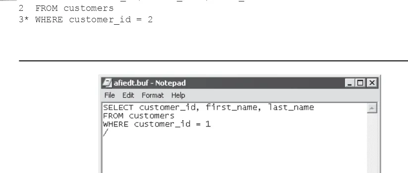
You can edit your last SQL statement in SQL*Plus by entering EDIT. Doing this is useful when you make a mistake or you want to make a change to your SQL statement. On Windows, when you enter EDIT you are taken to the Notepad application; you then use Notepad to edit your SQL statement. When you exit Notepad and save your statement, the new statement is
passed back to SQL*Plus, where you can re-execute it by entering a forward slash (/). On Linux or Unix, the default editor is typically set to vi or emacs.
NOTE
You’ll learn more about editing SQL statements using SQL*Plus in Chapter 3.
SQL Developer
You need to have Java installed on your computer before you can run SQL Developer. If you’re using Windows XP Professional Edition and Oracle Database 11g, you start SQL Developer by clicking Start and selecting All Programs | Oracle | Application Development | SQL Developer. SQL Developer will prompt you to select the Java executable. You then browse to the location where you have installed it and select the executable. Next, you need to create a connection by right-clicking Connections and selecting New Connection, as shown in the following illustration.
You can see full details on using SQL Developer by selecting Help | Table of Contents from the menu bar in SQL Developer.
In the next section, you’ll learn how to create the imaginary store schema used throughout this book.
Creating the Store Schema
The imaginary store sells items such as books, videos, DVDs, and CDs. The database for the store will hold information about the customers, employees, products, and sales. The SQL*Plus script to create the database is named store_schema.sql, which is located in the SQL directory where you extracted the Zip file for this book. The store_schema.sql script contains the DDL and DML statements used to create the store schema. You’ll now learn how to run the store_ schema.sql script.
Running the SQL*Plus Script to Create the Store Schema
You perform the following steps to create the store schema:
1. Start SQL*Plus.
2. Log into the database as a user with privileges to create new users, tables, and PL/SQL packages. I run scripts in my database using the system user; this user has all the required privileges. You may need to speak with your database administrator about setting up a user for you with the required privileges (they might also run the store_ schema.sql script for you).
3. Run the store_schema.sql script from within SQL*Plus using the @ command. The @ command has the following syntax:
@ directory\store_schema.sql
where directory is the directory where your store_schema.sql script is located. For example, if the script is stored in E:\sql_book\SQL, then you enter
@ E:\sql_book\SQL\store_schema.sql
If you have placed the store_schema.sql script in a directory that contains spaces, then you must place the directory and script in quotes after the @ command. For example:
@ "E:\Oracle SQL book\sql_book\SQL\store_schema.sql"
If you’re using Unix or Linux and you saved the script in a directory named SQL in the tmp
file system, then you enter
@ /tmp/SQL/store_schema.sql
NOTE
The first executable line in the store_schema.sql script attempts to drop the store user, generating an error because the user doesn’t exist yet. Don’t worry about the error: the line is there so you don’t have to manually drop the store user when recreating the schema later in the book.
When the store_schema.sql script has finished running, you’ll be connected as the
store user. If you want to, open the store_schema.sql script using a text editor like Windows Notepad and examine the statements contained in it. Don’t worry about the details of the statements contained in the script—you’ll learn the details as you progress through this book.
NOTE
To end SQL*Plus, you enter EXIT. To reconnect to the store schema in SQL*Plus, you enter store as the user name with a password of store_password. While you’re connected to the database, SQL*Plus maintains a database session for you. When you disconnect from the database, your session is ended. You can disconnect from the database and keep SQL*Plus running by entering DISCONNECT. You can then reconnect to a database by entering CONNECT.
Data Definition Language (DDL) Statements
Used to Create the Store Schema
As mentioned earlier, Data Definition Language (DDL) statements are used to create users and tables, plus many other types of structures in the database. In this section, you’ll see the DDL statements used to create the store user and some of the tables.
NOTE
The SQL statements you’ll see in the rest of this chapter are the same as those contained in the store_schema.sql script. You don’t have to type the statements in yourself: you just run the store_schema .sql script.
The next sections describe the following: How to create a database user
The commonly used data types used in an Oracle database Some of the tables in the imaginary store
Creating a Database User
To create a user in the database, you use the CREATE USER statement. The simplified syntax for the CREATE USER statement is as follows:
CREATE USER user_name IDENTIFIED BY password;
where
user_name is the user name
password is the password for the user
■ ■ ■
For example, the following CREATE USER statement creates the store user with a password of store_password:
CREATE USER store IDENTIFIED BY store_password;
If you want the user to be able to work in the database, the user must be granted the necessary permissions to do that work. In the case of store, this user must be able to log onto the database (which requires the connect permission) and create items like database tables (which requires the resource permission). Permissions are granted by a privileged user (for example, the system user) using the GRANT statement.
The following example grants the connect and resource permissions to store:
GRANT connect, resource TO store;
Once a user has been created, the database tables and other database objects can be created in the associated schema for that user. Many of the examples in this book use the store schema. Before I get into the details of the store tables, you need to know about the commonly used Oracle database types.
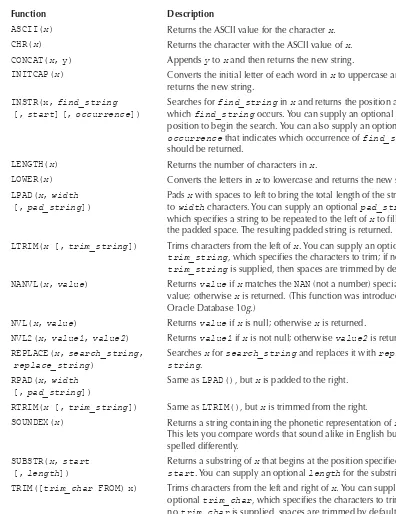
The Common Oracle Database Types
There are many types that may be used to handle data in an Oracle database. Some of the commonly used types are shown in Table 1-1.
You can see all the data types in the appendix. The following table illustrates a few examples of how numbers of type NUMBER are stored in the database.
Format Number Supplied Number Stored
NUMBER 1234.567 1234.567
NUMBER(6, 2) 123.4567 123.46
NUMBER(6, 2) 12345.67 Number exceeds the specified precision and is therefore rejected by the database.
Examining the Store Tables
In this section, you’ll learn how the tables for the store schema are created. Some of the information held in the store schema includes
Customer details Types of products sold Product details
A history of the products purchased by the customers Employees of the store
Salary grades
The following tables are used to hold the information:
customers holds the customer details.
product_types holds the types of products sold by the store.
■ ■ ■ ■ ■ ■
products holds the product details.
purchases holds which products were purchased by which customers.
employees holds the employee details.
salary_grades holds the salary grade details.
■ ■ ■ ■
Oracle Type Meaning
CHAR(length) Stores strings of a fixed length. The length parameter specifies the length of the string. If a string of a smaller length is stored, it is padded with spaces at the end. For example, CHAR(2) may be used to store a fixed-length string of two characters; if 'C' is stored in a CHAR(2), then a single space is added at the end;
'CA' is stored as is, with no padding.
VARCHAR2(length) Stores strings of a variable length. The length parameter specifies the maximum length of the string. For example, VARCHAR2(20)
may be used to store a string of up to 20 characters in length. No padding is used at the end of a smaller string.
DATE Stores dates and times. The DATE type stores the century, all four digits of a year, the month, the day, the hour (in 24-hour format), the minute, and the second. The DATE type may be used to store dates and times between January 1, 4712 B.C. and December 31, 4712 A.D.
INTEGER Stores integers. An integer doesn’t contain a floating point: it is a whole number, such as 1, 10, and 115.
NUMBER(
precision,
scale
)
Stores floating point numbers, but may also be used to store integers. The precision is the maximum number of digits (left and right of a decimal point, if used) that may be used for the number. The maximum precision supported by the Oracle database is 38. The scale is the maximum number of digits to the right of a decimal point (if used). If neither precision nor
scale is specified, any number may be stored up to a precision of 38 digits. Any attempt to store a number that exceeds the
precision is rejected by the database.
BINARY_FLOAT Introduced in Oracle Database 10g, stores a single precision 32-bit floating point number. You’ll learn more about BINARY_ FLOAT later in the section “The BINARY_FLOAT and BINARY_ DOUBLE Types.”
BINARY_DOUBLE Introduced in Oracle Database 10g, stores a double precision 64-bit floating point number. You’ll learn more about BINARY_ DOUBLE later in the section “The BINARY_FLOAT and BINARY_ DOUBLE Types.”
NOTE
The store_schema.sql script creates other tables and database items not mentioned in the previous list. You’ll learn about these items in later chapters.
In the following sections, you’ll see the details of some of the tables, and you’ll see the
CREATE TABLE statements included in the store_schema.sql script that create the tables.
The customers Table The customers table holds the details of the customers. The following items are held in this table:
First name Last name
Date of birth (dob) Phone number
Each of these items requires a column in the customers table. The customers table is created by the store_schema.sql script using the following CREATE TABLE statement:
CREATE TABLE customers (
customer_id INTEGER CONSTRAINT customers_pk PRIMARY KEY, first_name VARCHAR2(10) NOT NULL,
last_name VARCHAR2(10) NOT NULL, dob DATE,
phone VARCHAR2(12) );
As you can see, the customers table contains five columns, one for each item in the previous list, and an extra column named customer_id. The columns are
customer_id Contains a unique integer for each row in the table. Each table should have one or more columns that uniquely identifies each row; the column(s) are known as the primary key. The CONSTRAINT clause indicates that the customer_id column is the primary key. A CONSTRAINT clause restricts the values stored in a column, and, for the
customer_id column, the PRIMARY KEY keywords indicate that the customer_id
column must contain a unique value for each row. You can also attach an optional name to a constraint, which must immediately follow the CONSTRAINT keyword—for example, customers_pk. You should always name your primary key constraints, so that when a constraint error occurs it is easy to spot where it happened.
first_name Contains the first name of the customer. You’ll notice the use of the NOT NULL constraint for this column—this means that a value must be supplied for first_ name when adding or modifying a row. If a NOT NULL constraint is omitted, a user doesn’t need to supply a value and the column can remain empty.
■ ■ ■ ■
■
last_name Contains the last name of the customer. This column is NOT NULL, and therefore a value must be supplied when adding or modifying a row.
dob Contains the date of birth for the customer. Notice that no NOT NULL constraint is specified for this column; therefore, the default NULL is assumed, and a value is optional when adding or modifying a row.
phone Contains the phone number of the customer. This is an optional value. The store_schema.sql script populates the customers table with the following rows:
customer_id first_name last_name dob phone
--- --- --- --- 1 John Brown 01-JAN-65 800-555-1211 2 Cynthia Green 05-FEB-68 800-555-1212 3 Steve White 16-MAR-71 800-555-1213 4 Gail Black 800-555-1214 5 Doreen Blue 20-MAY-70
Notice that customer #4’s date of birth is null, as is customer #5’s phone number. You can see the rows in the customers table for yourself by executing the following
SELECT statement using SQL*Plus:
SELECT * FROM customers;
The asterisk (*) indicates that you want to retrieve all the columns from the customers table.
NOTE
In this book, SQL statements shown in bold are statements you should type in and run if you want to follow along with the examples. Non-bold statements are statements you don’t need to type in.
The product_types Table The product_types table holds the names of the product types sold by the store. This table is created by the store_schema.sql script using the following CREATE TABLE statement:
CREATE TABLE product_types (
product_type_id INTEGER CONSTRAINT product_types_pk PRIMARY KEY, name VARCHAR2(10) NOT NULL
);
The product_types table contains the following two columns:
product_type_id uniquely identifies each row in the table; the product_type_id
column is the primary key for this table. Each row in the product_types table must have a unique integer value for the product_type_id column.
name contains the product type name. It is a NOT NULL column, and therefore a value must be supplied when adding or modifying a row.
■
■
■
■
The store_schema.sql script populates the product_types table with the following rows:
product_type_id name --- 1 Book 2 Video 3 DVD 4 CD 5 Magazine
The product_types table contains the product types for the store. Each product sold by the store must be one of these types.
You can see the rows in the product_types table for yourself by executing the following
SELECT statement using SQL*Plus:
SELECT * FROM product_types;
The products Table The products table holds the products sold by the store. The following pieces of information are held for each product:
Product type Name Description Price
The store_schema.sql script creates the products table using the following CREATE TABLE statement:
CREATE TABLE products (
product_id INTEGER CONSTRAINT products_pk PRIMARY KEY, product_type_id INTEGER
CONSTRAINT products_fk_product_types REFERENCES product_types(product_type_id), name VARCHAR2(30) NOT NULL,
description VARCHAR2(50), price NUMBER(5, 2)
);
The columns in this table are as follows:
product_id uniquely identifies each row in the table. This column is the primary key of the table.
product_type_id associates each product with a product type. This column is a reference to the product_type_id column in the product_types table; it is known as a foreign key because it references a column in another table. The table containing the foreign key (the products table) is known as the detail or child table, and the table that is referenced (the product_types table) is known as the master or parent table.
■ ■ ■ ■
■
This type of relationship is known as a master-detail or parent-child relationship. When you add a new product, you associate that product with a type by supplying a matching
product_types.product_type_id value in the products.product_type_id
column (you’ll see an example later).
name contains the product name, which must be specified, as the name column is
NOT NULL.
description contains an optional description of the product.
price contains an optional price for a product. This column is defined as NUMBER(5, 2)—the precision is 5, and therefore a maximum of 5 digits may be supplied for this number. The scale is 2; therefore 2 of those maximum 5 digits may be to the right of the decimal point.
The following is a subset of the rows stored in the products table:
product_id product_type_id name description price --- -- -- 1 1 Modern A 19.95 Science description
of modern science
2 1 Chemistry Introduction 30 to Chemistry
3 2 Supernova A star 25.99 explodes
4 2 Tank War Action movie 13.95 about a
future war
The first row in the products table has a product_type_id of 1, which means the product is a book (this product_type_id matches the “book” product type in the product_types
table). The second product is also a book, but the third and fourth products are videos (their
product_type_id is 2, which matches the “video” product type in the product_types table). You can see all the rows in the products table for yourself by executing the following
SELECT statement using SQL*Plus:
SELECT * FROM products;
The purchases Table The purchases table holds the purchases made by a customer. For each purchase made by a customer, the following information is held:
Product ID Customer ID
Number of units of the product that were purchased by the customer
■
■ ■
The store_schema.sql script uses the following CREATE TABLE statement to create the
purchases table:
CREATE TABLE purchases ( product_id INTEGER
CONSTRAINT purchases_fk_products REFERENCES products(product_id), customer_id INTEGER
CONSTRAINT purchases_fk_customers REFERENCES customers(customer_id), quantity INTEGER NOT NULL,
CONSTRAINT purchases_pk PRIMARY KEY (product_id, customer_id) );
The columns in this table are as follows:
product_id contains the ID of the product that was purchased. This must match a
product_id column value in the products table.
customer_id contains the ID of a customer who made the purchase. This must match a customer_id column value in the customers table.
quantity contains the number of units of the product that were purchased by the customer.
The purchases table has a primary key constraint named purchases_pk that spans two columns: product_id and customer_id. The combination of the two column values must be unique for each row. When a primary key consists of multiple columns, it is known as a
composite primary key.
The following is a subset of the rows that are stored in the purchases table:
product_id customer_id quantity - 1 1 1 2 1 3 1 4 1 2 2 1 1 3 1
As you can see, the combination of the values in the product_id and customer_id columns is unique for each row.
You can see all the rows in the purchases table for yourself by executing the following
SELECT statement using SQL*Plus:
SELECT * FROM purchases;
The employees Table The employees table holds the details of the employees. The following information is held in the table:
Employee ID
■
■
■
The ID of the employee’s manager (if applicable) First name
Last name Title Salary
The store_schema.sql script uses the following CREATE TABLE statement to create the
employees table:
CREATE TABLE employees (
employee_id INTEGER CONSTRAINT employees_pk PRIMARY KEY, manager_id INTEGER,
first_name VARCHAR2(10) NOT NULL, last_name VARCHAR2(10) NOT NULL, title VARCHAR2(20),
salary NUMBER(6, 0) );
The store_schema.sql script populates the employees table with the following rows:
employee_id manager_id first_name last_name title salary - --- 1 James Smith CEO 800000 2 1 Ron Johnson Sales Manager 600000 3 2 Fred Hobbs Salesperson 150000 4 2 Susan Jones Salesperson 500000
As you can see, James Smith doesn’t have a manager. That’s because he is the CEO of the store.
The salary_grades Table The salary_grades table holds the different salary grades available to employees. The following information is held:
Salary grade ID
Low salary boundary for the grade High salary boundary for the grade
The store_schema.sql script uses the following CREATE TABLE statement to create the
salary_grades table:
CREATE TABLE salary_grades (
salary_grade_id INTEGER CONSTRAINT salary_grade_pk PRIMARY KEY, low_salary NUMBER(6, 0),
high_salary NUMBER(6, 0) );
■ ■ ■ ■ ■