MITIGATION OF FLASH FLOODS IN ARID REGIONS USING ADJOINT SENSITIVITY ANALYSIS
Hossam Elhanafy *, Graham J.M. Copeland **.
ABSTRACT:
This paper presents an analysis of the sensitivities of flood wave propagation to variations in certain control variables and boundary conditions by means of the adjoint method. This uses a variational technique to find the relationships between changes in predicted flood water levels and changes in control variables such as the inflow hydrograph, bed roughness, and bed elevation. The sensitivities can be used for optimal control of hydraulic structures, for data assimilation, for decision makers' procedures, for the analysis of the effects of uncertainties in control variables on the predictions of floods water levels, and for investigating both the sensitivities of model flood forecasts to model parameters, boundary and initial conditions.Example of the last application of the sensitivity analysis is presented and discussed
These methods are developed and implemented through a numerical hydraulic model of channel flow based on the Shallow Water Equations (SWEs) and the corresponding adjoint model. The equations are integrated using finite difference methods and a new modified method of characteristics is used to define the open boundaries. Results of validation tests on both the forward hydraulic model and on the adjoint model are presented.
Keywords
Open channel flow; Adjoint sensitivity analysis; Numerical models; Flash floods.
* PhD student, Civil Engineering Department, Strathclyde University, Scotland, U.K.
** Reader, Civil Engineering Department, Strathclyde University, Scotland, U.K.
INTRODUCTION:
are the values of the inflow hydrograph, downstream water level, bed roughness, and bed slope. This paper presents an analysis of how a model prediction of flood water level at a certain location is sensitive to variations in some of these control values. These sensitivities can be used to select the most appropriate location and rate of abstraction for flood control, Ding & Wang [4], to optimize water abstraction for irrigation, Sanders & Katapodes [3] or to identify Manning's roughness coefficient, Ding et al. [5]. The sensitivities can also be used for data assimilation, Cacuci [6] and Navon [7] and to quantify the consequential effects of sensitivities in some control values on predicted flood levels or flood volume as shown in this paper.
The adjoint sensitivity analysis has been implemented through the development of two numerical models; a forward model, based on the nonlinear Shallow Water Equations (SWEs) used to simulate the propagation of the flood wave, and an adjoint model used to evaluate the time-dependent sensitivities with respect to a variety of control variables under different flow conditions. The adjoint method requires that the forward problem and its associated adjoint problem are solved sequentially. Sensitivity expressions which are functions of the forward and adjoint variables can be applied to assess the change in outcome resulting from changes in control values. The adjoint sensitivity analysis is used here to establish relationships between certain controls and the system responses. A particular control problem is defined by selection of an appropriate objective function. This may require to be minimized in the case of data assimilation or, for example, it may measure flood water levels in excess of some threshold as discussed in this paper. Once this objective function is defined, the adjoint sensitivity analysis is used to evaluate the gradient of this function with respect to the control variables or in other word the sensitivities.
1. GOVERNING EQUATIINS FOR THE OPEN CHANNEL FLOW:
The one dimensional Shallow Water Equations (SWEs) form a system of partial differential equations which represents mass and momentum conservation along the channel and include source terms for the bed slope and bed friction. These equations may be written as:
0 = ∂ ∂ + ∂ ∂
x q t
H
(1)
0 ) ( )
( 0 =
∂ ∂ + − −
∂ ∂ + ∂ ∂
x qu S
S gH x H gH t
q
f (2)
Where:
q : is the discharge per unit width (m2s-1). g : is the gravitational acceleration. H : is the total water depth
S0 : is the bed slope = - x
z
∂ ∂
.
t : is the time (s).
x : is the horizontal distance along the channel (m). Sf : is the bed friction slope = gH3
q q k
k : is a friction factor = g/C2 according to Chezy or = gn2/ H(1/3) according to Manning .
x qu ∂ ∂( )
: is the momentum flux term, or convective acceleration
In simulating an unsteady channel flow during a flood wave event the one dimensional SWEs, Equation (1) and Equation (2) are subjected to initial and boundary conditions. Initial conditions are q(x,0) and H(x,0) and the boundary conditions are q(0,t) and H(L,t) where x = L is the downstream limit of the model domain. Values q(0,t) comprise the inflow hydrograph and H(L,t) are interpolated from within the domain using the method of characteristics (MOC), Abbott [13] and French [14] after modifying it to suit the case of sloping rough bed described below to provide a transparent downstream boundary through which the flood wave can pass without reflection.
2. ADJOINT SENSTIVITY ANALYSIS FOR THE (SWEs): 2.1. Defining the objective function:
If the application of the analysis is to the control or assessment of risk of flood water levels then it is convenient to compare predicted levels with known threshold values above which flooding could occur. A measure of the difference between these levels can be used to quantify the effect of a control. In particular, we are interested in water levels that exceed threshold values at certain locations (xo) and at certain times (to). As a surrogate for level we can
use local depth H (provided the local bed level z is known) and so define a quadratic objective function that quantifies the water depths greater then some specified threshold flood depths H d.
r = 0.5{(H - H d) │ H - H d│} δ(x – xo) δ(t – to) (3)
Where:
H (x, t) is the water depth calculated by the forward hydraulic model, and H d (xo, to) are threshold values at x = x o, and t = to.
2.2. Governing equation for the sensitivity analysis:
Adjoint sensitivity analysis evaluates the sensitivities of the objective function to certain control variables. This is achieved by creating the Lagrangian and taking the first variation. The method follows closely that described by Sanders & Katopodes [3], Gejadze & Copeland [8], and Copeland& El-hanafy [9] as follow:
∫ ∫
∂ ∂ + − − ∂ ∂ + ∂ ∂ + ∂ ∂ + ∂ ∂ += T L
f dt dx x qu S S gH x H gH t q x q t H r J 0 0 0 ) ( ) ( ψ φ (4)
where the weights φ and ψ are Lagrange multipliers later to be revealed as the adjoint variables. The sensitivities and the adjoint equations are evaluated by taking the first variation of J in Equation (4) with respect to all flow
variables and control variables, taking into consideration that x z
∂ ∂
= -So,
qu=
H q2
, Sf = 3 gH
q q
k , 2
C g
k= and using integration by parts, the final
expression for the variation in J ,δJ , is given by the sum of the following 6 integrals:-
[
]
{
}
(
)
dt dx z g H z g dt dx C H C q q g dt dx q q r x H q H C q g x t H H r x H q H C q q g x z g x gH t dt z gH H gH H H q q H q q dx q H J T L T L T L L T T L δ ψ δ ψ δ ψ ψ φ ψ δ ψ ψ ψ ψ φ δ ψ δ ψ δ ψ δ ψ δ φ δ ψ δ φ δ∫ ∫
∫ ∫
∫ ∫
∫
∫
∂ ∂ − − + ∂ ∂ + ∂ ∂ − + ∂ ∂ − ∂ ∂ − + ∂ ∂ + ∂ ∂ + − ∂ ∂ + ∂ ∂ − ∂ ∂ − + + + − + + + = 0 00 0 3 2
2 2 2 2 3 2 0 0 0 2 0 0 0 2 2 2 2 2
We are seeking variations in J that are caused by possible variations in q and H as the initial conditions and at the upstream and downstream boundaries. We also are looking for the effects of variations in controls C, and Z in the domain. These are expressed by integrals 1, 2, 4, and 5 respectiveley in Equation (5). We are not looking for the effects of variations in q and H within the domain as expressed by integral 3 in Equation (5). Hence this integral is required to equal zero for any variations in q and H. This conditions leads to the identification of the two adjoint equations from the kernal of this integral as follows:- 0 2 2 2 3 2 = ∂ ∂ + ∂ ∂ + − ∂ ∂ + ∂ ∂ − ∂ ∂ H r x H q H C q q g x z g x
gH ψ ψ ψ ψ
τ φ
0 2
2 2 2 =
∂ ∂ + ∂ ∂ − + ∂ ∂ − ∂ ∂ q r x H q H C q g x ψ ψ φ τ ψ Where τ = (T – t), measured in reverse time direction.
Solution of adjoint equations, Equation (6), for given flow conditions q and H ensures that integral 3 in Equation (5) equals zero and provides values for φ
and ψ everywhere in the domain. These values can be used in conditions derived from integrals 1, 2, 4, and 5 in Equation (5) to quantify the sensitivitiesas shown below.
2.3. Derivation of the sensitivities:
2.3.1. Sensitivity to the upstream channel flow:
Sensitivities to initial condtions are revealed by integral 1 in Equation (5). If we impose the conditions φ(x,T) = ψ(x,T) = 0, that is no sensitivity information propagates into the domain at t = T, then the sensitivity to initial
conditions is just φ δ
δ
− = ) 0 , (x H
J
and ψ
δ δ
− = ) 0 , (x q
J
at each discrete location
along the channel. If we do not want to control the solution to any initial condition then we may set δq(x,0)=δH(x,0)= 0 then integral 1 vanishes. Sensitivities to boundary conditions are revealed by integral 2 in Equation (5). If we impose the condition δq(L,t) = 0, that is q(L,t) is not used as a control, then the sensitivity to inflow q(0,t) is shown to be
{
(0, ) 2 (0, ) (0, )}
), 0
( tp tp u tp tp
q J
ψ φ
δ δ
+ −
= (7)
at each time step or perturbation time from t = 0 to T.
Similarly by imposing condition δH(0,t) = 0, that is H(0,t) is not used as a control, then the sensitivity to downstream depth H is shown to be
( )
{
( , ) ( , ) ( , )}
( , ) ), (
2
p p
p p
p
t L t L u t L H t L g t L H
J
ψ δ
δ
−
= (8)
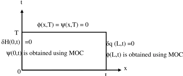
Figure (1) shows all of the required boundary conditions. We note that the boundary conditions for ψ(0,t) and φ(L,t) are both required and must be defined such that both boundaries are transparent to the outgoing peturbations created within the adjoint domain. This is achieved by interpolation from available values within the domain using the method of characteristics (MOC), the formulation will be given below.
Figure (1) Boundaries and initial conditions for the solution domain 2.3.2. Sensitivity to the Bed elevation:
The bed elevation can be considered as a control variable which can affect the flood level at x = xo. Sensitivities to the bed elevation at both the upstream
and boundary conditions are revealed by integral 2 in Equation (5). If we x
t
L 0
T
φ(x,T) = ψ(x,T) = 0
δH(0,t) =0
ψ(0,t) is obtained using MOC
δq (L,t) =0
[image:5.612.179.498.503.637.2]impose the condition δZ(L,t) = δZ(0,t) =0, that is Z(L,t) and Z(0,t) are not used as a control, then the sensitivity with respect to the bed elevation within the whole domain, from integral 6 in Equation (5), is written as:
(
)
dt dx x H z g zJ T L
∫ ∫
∂∂ − = 0 0 ψ δ δ (9)From Equation (9) the spatial and temporal variations of the sensitivity with respect to the bed elevation can be evaluated after the two adjoint equations, Equation (6) are solved.
2.3.3. Sensitivity to the Bed friction:
The bed friction, in terms of Chezy coefficient can be also considered as a control variable which should affect the flood level, hence the sensitivity is written as: dt dx H C q q g C
J T L
∫ ∫
− =0 0 2ψ 3 2
δ δ
(10)
From Equation (10) the spatial and temporal variations of the sensitivity with respect to Chezy coefficient can be evaluated after the two adjoint equations, Equation (6) are solved
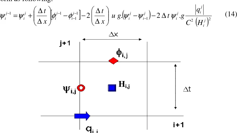
3. NUMERICAL APPROACH: 3.1. Discretising the Forward Model:
The finite difference mesh for discretising the domain is depicted in Figure (2) that follows a simple space and time staggered. A regular mesh of dimension (∆x), spacing of grid points in x-direction by (∆t), spacing in the time direction, so now if [0,L] is discretised by (nx) equally spaced then
1 nx − =
∆x L , and by the same concept
1 − = ∆ nt T
t , so the discretised values of
a function (h) at (i ∆x , j ∆t) will be denoted hij= h(i,j) = h(i ∆x,j ∆t) the
superscription (j) refer to time discretization and is called time step or time level, while the subscript (i) refers to space discretization and is called space
step or space level. The approximation of the derivatives ∂∂hx is now
x j i h j i h ∆ − −
1 ,a first order upwind scheme is used to stabilize the solution of
the shallow water equation, the convective term ∂(∂qux ) is discretised with two point upwind difference expression or a weighted average of centered and upwind difference expressions:
(
)
x i qu i qu i qu i qu x i qu i qu x qu ∆ + − + − − − + ∆ − − + = ∂ ∂ 3 ) 1 ( ) ( 3 ) 1 ( 3 ) 2 ( 5 . 0 2 ) 1 ( ) 1 ( ) ([
]
x qu t H q q k t z z x t gH H H x t gH q q j i j i j i i i j i j i j i j i j i j i ∂ ∂ ∆ − ∆ − − ∆ ∆ − − ∆ ∆ − = − − + ( ) . ) ( . . ) ( .. 1 1 2
1
(11)
The water depth H is marched forward in time using the continuity equation:
[
1 1]
1
1 + +
+ + − ∆ ∆ − = j i j i j i j
i q q
x t H
H (12)
The initial conditions are H1i and 1 i
q while the boundary conditions are 1 1
+
j
q
at the upstream boundary and Hnxj+1 at the downstream boundary, the upstream
condition is the inflow hydrograph; the downstream condition must be interpolated using the method of characteristics (MOC) as described in Abbott [13] and French [14].
3.2. Discretising the Adjoint Model
The adjoint model which is represented by Equation (6) is discretized using a simple space and time staggered explicit finite difference scheme as illustrated in Figure (2). The adjoint variable φ is marched backwards in time using the discrete form as following
[
]
(
)
32 1 1 2 2 1 . 2 . . ). ( j i j i j i j i i i j i j i j i j i j i H C q q g t z z x t g x t u
c ψ ψ ψ ψ
φ
φ − + ∆
∆ ∆ − − ∆ ∆ − + = + − − (13)
While the adjoint variable ψ is marched backwards in time using the discrete form as following:
[
]
(
)
( )
2 2 1 1 1 1 1 . 2 . 2 j i j i j i j i j i j i j i j i j i H C q g t g u x t x t ψ ψ ψ φ φ ψψ − − ∆
∆ ∆ − − ∆ ∆ + = − − − − −
Figure (2) The discretization scheme for the forward and adjoint model
3.3. Method Of Characteristics (MOC):
Following a standard text such as Abbott [13] and French [14], the characteristics of the linearized (SWEs) are identified as:
H
i,j [image:7.612.114.505.404.624.2]0 )
( 2 =
∂ ∂ + +
∆ ± − ∆
x z gH H
q q K H c u
q (15)
While characteristics of the adjoint model are identified as:
0 ) 2
)( ( 2
)
( 2 3 + ± 2 2 =
∂ ∂ + −
∆ ± + ∆
H C
q g c
u x z g H C
q q g c
u ψ ψ ψ ψ
φ (16)
Where ∆ indicates a total change in variable along the characteristic path.
4. MODELS VERIFICATIONS: 4.1. Forward model verifications:
4.1.1 Introduction:
Developing a complete test to check and validate an exact solution for the nonlinear Shallow Water Equations (SWEs) is not possible. It is possible however to develop simple tests to compare the model results with analytical solutions of certain idealized cases. Several tests have been carried out to verify the model from uniform steady flow to non-uniform unsteady flow; we will mention here just the two most important tests.
4.1.2 Validation test 1 – non-uniform unsteady flow:
The main objectives of this test are to assure the following:
- The value of both the discharge (q) and the water depth (H) at the upstream propagate downstream without any change.
- The relationship between q and H follow the analytical solution of the shallow water wave.
The analytical solution of the shallow water wave:
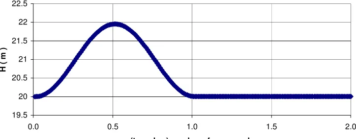
The analytical solution of the shallow water equation in deep water initially, 20 m. with a driving upstream hydrograph following sinusoidal wave concept of amplitude 2.0 m.as illustrated at Figure (3), where; a: is the amplitude of the wave, T: is wave period, t: time, c: wave speed = √ g.H. , and H: is the total water depth is η = a .{1+ sin(θ)} = 2.0 m which lead to H max= 22.0 m and q = a . √ (g. H). (1+sin (Θ)) + q 0 which lead to q max= 28.01 m3/s/m. and the
traveling speed is equal to √ (g. H) = 14.69 m/s
19.5 20 20.5 21 21.5 22 22.5
0.0 0.5 1.0 1.5 2.0
(t_cycles ) number of wave cycle
H
(
m
)
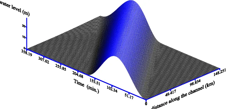
[image:8.612.126.488.542.684.2]The results of the model are a driving upstream boundary hydrograph of peak discharge q = 28.24 m3/s/m and the calculated upstream boundary hydrograph of peak value, H max = 21.96 m. while the wave speed is 14.74 m/s. so, the first conclusion is that the relationship calculated by the model typically follow the shallow wave equation and although there is discrepancy between the calculated values from the model and the analytical solution but this discrepancy could be interpreted due to the values of distance step = 3.025 Km and time step of 108 s, the second conclusion is that the hydrograph traveled from the upstream boundary to the down stream boundary with a small change in the peak discharge from 28.01 m3/s/m to 28.24 m3/s/m and from 21.96 m to 21.94 m for the peak water depth as illustrated at Figure (4) and this acceptable diffusion is duo to the numerical dissipation of the used explicit scheme. The last conclusion is that the wave traveled a distance of 151.26 Km. within 10260 sec. so its speed is 14.74 m/s. while the speed of the wave should equal to √ (g. H) = 14.69 m/s which is nearly the same. So finally, it is clear there is a good agreement between the analytical solution and the developed model and also there is no numerical dissipation.
Figure (4) Water depth (H) within the domain
4.1.3 Validation test 2 - Unsteady flow within a sloping channel and rough bed:
There are two main objectives of this test; the first objective is simply to look for the whole channel as a control volume to assure there is no significant losses or accumulation in volume within the simulated domain and the results of this tests will not be compared with the analytical solution only, but will be compared with other model results as well, the second objective is to assure the volumetric conservation principal at different time steps is always valid and no numerical oscillation at the wave front. If we considered the initial water depth is Hi and at the end of the simulation is Hf. While the driving discharge
[image:9.612.112.508.340.527.2]Total volume enters the channel is ∆V1 =
∫
qu dt−∫
qd dt, while the total volume leaves the channel is ∆V2 =∫
Hf dx−∫
Hi dx, to be in equilibrium, it should be2
1 V
V =∆
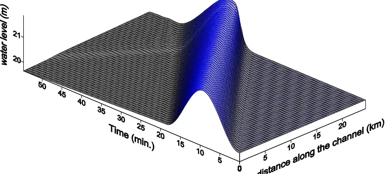
∆ . The model was applied for non-uniform unsteady flow conditions within a slopping channel and rough bed. The initial water depth was chosen H initial = 20.0 m. The result of the flood wave propagation within the domain is presented at Figure (5).
Figure (5) Water depth (H) within the domain
95 . 5284 63
. 2740 3 58 . 8025 3
1 = − = − =
∆V
∫
qd dt∫
qu dt m3/m36 . 5330 494669.64
00000 5
2 = − = − =
∆V
∫
Hi dx∫
Hf dx m3/mSo, ∆V2−∆V1 ≅45.41 m3 ≈ 0.86 ٪ which is acceptable and it is very small error compared to several previously developed model such as Abiola [15] which was overestimates by 28 %.
4.2. Adjoint verifications:
In the following experiment, a direct simulation is done first with a chosen boundary q1 and the results at certain location are now considered as the
observations q1(x = x0). Then the model is re-run again with a new boundary q2
and the results at same location are recorded q2(x = x0). The discrepancy
between the two solutions at (x = x0) is used to measure the cost function. Then
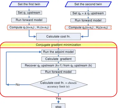
by using the conjugate gradient minimization the cost function is minimized at each iteration to cover q1 from q2 as shown in Figure (6). This technique where
[image:10.612.112.506.207.382.2]Run forward model Set q1 upstream
Run forward model Set q2 = a q1 upstream
Calculate cost fn.
Run the adjoint model
Recover q2 upstream (k+1) from q2 upstream (k)
Run forward model Calculate cost fn. = chosen
accuracy limit (e)
stop Yes No
Conjugate gradient minimization
Set the first twin Set the second twin
Compute q1(x=x0) , H1(x=x0) Compute q2(x=x0) , H2(x=x0)
Calculate gradient
Figure (6) Identical twin experiment flow chart
The convergence was rapid that the inlet hydrograph, q1 was found after
only 14 iterations that a reduction of the measuring function by a factor 100000 was achieved in about 10 iterations and about 97 % of q1 had been recovered
after only three iterations as illustrated in Figure (7) and Figure (8).
0.00000001 0.0000001 0.000001 0.00001 0.0001 0.001 0.01 0.1 1 10
0 5 10 15
no. of iterations
c
o
s
t
fu
n
c
ti
o
n
[image:11.612.115.500.64.414.2] [image:11.612.121.489.518.679.2]17 19 21 23 25 27 29 31
0 0.1 0.2 0.3 0.4 0.5 0.6 0.7 0.8
Time (Hours.)
W
a
te
r
le
v
e
l
(m
)
Iteration=1 Iteration=2 Iteration=3
Hydrograph at inlet ,(q2)
,(q1)
Figure (8) recovering of q1 from q2 as a result of
The identical twin experiment. 4. TEST CASE:
In this case, a 30 Km-long channel with an upstream hydrograph following a sinusoidal wave shape as shown in Figure (3) that will be used to run the forward model and then the adjoint equations (6) are solved, the values of the adjoint variables [φ, ψ] are then obtained within the whole domain as shown in Figure (9) .
A – φ B – ψ
Figure (9) Solution of the adjoint variables [φ, ψ]
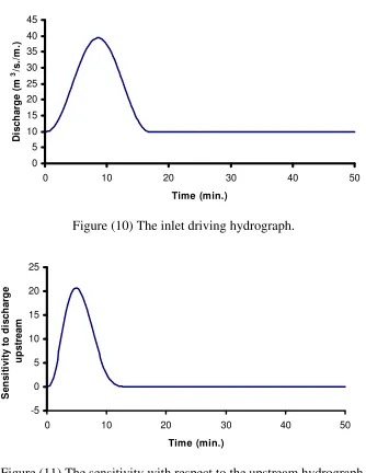
[image:12.612.122.489.75.301.2] [image:12.612.97.510.102.635.2] [image:12.612.95.517.415.635.2]discharge described in Equation (7), the temporal variation of the sensitivity (0, )
p
t q
J
δ δ
is shown in Figure (11) which is consistent to the driving hydrograph upstream, shown in Figure (10)
0 5 10 15 20 25 30 35 40 45
0 10 20 30 40 50
Time (min.)
D
is
c
h
a
rg
e
(
m
3 /s
./
m
.)
Figure (10) The inlet driving hydrograph.
-5 0 5 10 15 20 25
0 10 20 30 40 50
Time (min.)
S
e
n
s
it
iv
it
y
t
o
d
is
c
h
a
rg
e
u
p
s
tr
e
a
m
Figure (11) The sensitivity with respect to the upstream hydrograph.
The variations of the sensitivity to the bed elevation described in Equation (9),
z J δ δ
in
space and time is shown in Figure (12). While the variations of the sensitivity with
respect to the Chezy coefficient described in Equation (10), C J
δ δ
in space and time is
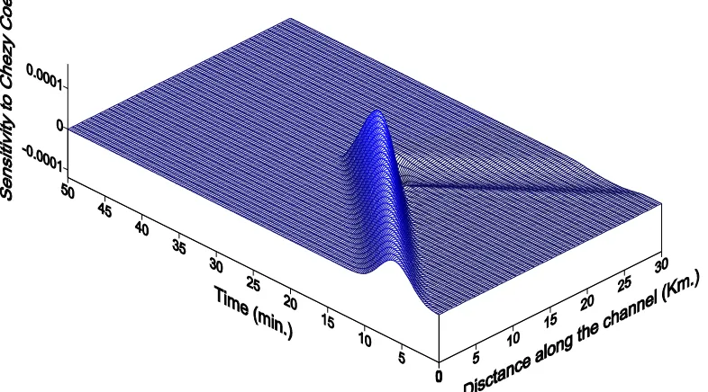
[image:13.612.138.472.129.561.2] [image:13.612.149.466.144.312.2]Figure (12) The sensitivity with respect to the bed elevation.
Figure (13) The sensitivity with respect to Chezy Coefficient.
5. CONCUSIONS:
[image:14.612.111.505.73.287.2] [image:14.612.112.505.365.583.2]in other word the sensitivity increases as the discharge increases and decreases as the discharge decreases. While the sensitivity to the bed elevation which is illustrated in Figure (12) explain the effect of the bed elevation from the upstream boundary to the down stream boundary on the threshold water level. Finally, Figure (13) show that the effect of the channel roughness from the upstream boundary till the specified location (x0) is much more greater than
from the specified location (x0) till the down stream boundary duo to the
backwater effect that agree with the basic hydraulic concepts in that any information could propagate upstream only in subcritical flow, which is case studied in this paper. These sensitivities could now be functioned for several purposes, it could be used for parameters identification or it could be used by decision makers to help in prioritizing the most important parameters, in the case studied in this paper as an example, it is clear that the most important control variable is the driving upstream discharge compared to the bed elevation and the channel roughness expressed in Chezy coefficient. or it may be used as a tool to mitigate the flood hazards at certain locations along the channel by identifying the threshold water level not only at x = (x0) but as
function along the studied channel and select the most appropriate location for a certain control action which may be a reservoir or detention dam or a diversion channel. The proper numerical solution and achieving open boundaries for both the forward model and the adjoint problem lead to formulation of an adjoint solution which is consistent with the basic problem. In the near future, the research is to be extended to evaluate both the effect of individual uncertainty in each control variable on the flood event and the global uncertainty from all the control variables on the flood impact.
ACKNOWLEDGMENTS
The authors would like to express their deepest gratitude to Dr. Igor Gejadze for his sincere concern and useful guidance through my PhD research.
I am particularly appreciating my sponsor at my country who gave me this chance to complete my study.
Last but not least, I would like to thank all my colleagues and the staff of civil engineering department of Strathclyde University.
REFERENCES:
1 Effect Of Environmental Changes On Drainage Patterns And Urban Planning Along Coastal Regions (Case Study), (Moussa, O.M., Abdelmetaal, N.H., Elmongy, A.E, .and EL-Hanafy, H.M.), pp. 1-17, Third International Conference On Civil & Architecture Engineering , Military Technical College , Kobry Elkobbah, Cairo Egypt, SU9, 1999.
2 Control of multi-dimensional wave motion in shallow-water, (Sanders, B.F and Katopodes, N.D.), 267-278, Proceedings of the 5th Int. Conf. on Estuarine and Coast. Modeling, M. L. Spaulding, ed., 1998
4 Ding, Y. and Wang, S.Y., Optimal control of open-channel flow using adjoint sensitivity analysis, Journal of Hydraulic Engineering, ASCE, vol. 132, no. 11, pp 1215-1228
5 Ding, Y., Jia Y., and Wang, S.Y., Identification of Manning's roughness coefficients in shallow water flows, Journal of Hydraulic Engineering, ASCE, vol. 130, no. 6, in press.
6 Cacuci, D.G., Chapter 3, Sensitivity and Uncertainty Analysis, Volume I, Chapman & Hall CRC., 2003
7 Application of the Adjoint Model in Meteorology, (Navon, I.M. and Zou, X.) Proceedings of the International Conference on Automatic Differentiation of Algorithms: Theory, Implementation and Application, SIAM Publications, A. Griewanek and G. Corliss Eds, SIAM, Philadelphia, PA 1991.
8 Gejadze, I.Yu and Copeland, G.J.M., Adjoint sensitivity analysis for fluid flow with free surface, Int. J. Numer. Methods in Fluids, vol 47, Issue 8-9,pp 1027-1034.
9 Computer modelling of channel flow using an inverse method, (Copeland, G.J.M. & El-Hanafy, H.), Proc. 6th Int. Conf. on Civil and Arch. Eng, Cairo, May 2006.
10 Fletcher, C.J., Chapter 5, Computational Techniques for Fluid Dynamics 1: Fundamental and General Techniques, Springer-Verlang., 1991
11 Leonard, B.P., Third-Order Upwinding as a Rational Basis for Computational Fluid Dynamics, Computational Techniques & Applications: CTAC-83, Edited by Noye, J. And Fletcher, C., Elsevier.
12 Falconer, R.A. and Liu, S.Q., Modeling Solute Transport Using QUICK Scheme, ASCE Journal of Environmental Engineering, vol. 114, pp. 3-20. 13 M.B. Abbott, Chapter 2&3, An Introduction to the method of characteristics,
Thames and Hudson,London UK, 1977.
14 French, R.H. Chapter 4&6, Open Channel Hydraulics, McGraw Hill,1986. 15 Abiola, A.A. and Nikaloaos, D.K., Model for Flood Propagation on Initially