Coastal morphodynamical modelling in nonlinear shallow water framework using a coordinate transformation method

Coastal morphodynamical modelling in nonlinear shallow water framework

using a coordinate transformation method

Van Long Huynha,∗, Nicholas Dodda_{, Fangfang Zhu}b

a_{Faculty of Engineering, University of Nottingham, NG7 2RD, UK}

b_{University of Nottingham Ningbo China, 315100}

Abstract

A 1D numerical model of Nonlinear Shallow Water Equations (NSWEs) coupled to an advection equation for suspended sediment and a bed evolution equation is developed. The moving boundary at the shore-line is treated by a coordinate transformation method (CTM). An absorbing-generating seaward boundary condition in the transformed variables is also developed. The purely hydrodynamic component (NSWEs) is verified against analytical results. The NSWEs plus advection equation is verified quasi-analytical re-sults. The fully-coupled model with bed change due to bed-load is verified against a single swash event and long-term numerical simulation. Excellent agreement is observed in all verifications.

Keywords: Coupled hydro-morphodynamic model; Coordinate transformation method; Non-breaking waves; Wetting-drying

1. Introduction

Hydrodynamics in a shallow water region such as the nearshore zone can be well described by the Nonlinear Shallow Water Equations (NSWEs). These equations describe well water motion in which the velocity can be considered mostly depth-invariant [1]. In simplifying but still adequately describing the fundamental physical phenomena, and thereby allowing a more rapid numerical solution, the NSWEs possess

5

distinct advantages over more comprehensive equation sets, such as the Euler equations, for modelling breaking and non-breaking long waves such as waves in the swash and inner surf zones and tidal motions [2]. The domain of NSWEs is typically bounded by a free-moving boundary at the shoreline and an absorbing-generating boundary at the offshore. The most challenging problem related to modelling NSWEs is properly describing the free-moving boundary at the shoreline.

10

In numerical models, proper definition of the shoreline boundary is crucial for implementing an efficient and robust model. Many methodologies have been applied in order to accommodate the free moving bound-ary. Most of these implement the moving shoreline on a fixed computational grid in which the shoreline position is located either at a grid point [3], [4] or extrapolated to some point between the grid points [5], [6]. Typically there is a threshold value that defines the wet-dry interface and determines where the shoreline

15

is located. Arguably, a more mathematically elegant approach is to use a coordinate transformation to map the moving domain onto a fixed one, thus the governing equations must be transformed into the new coordinates. [7] solved the 1DH NSWEs by mapping the fluid domain onto a fixed domain and applied linear extrapolation of water surface elevation to obtain the shoreline position. A similar technique was applied by [8] with a semi-characteristic method to reduce the need of one-sided approximation at the shore. [9]

20

obtained 2DH NSWEs in a partial characteristics form and solved on a transformed domain, in which the spatial derivatives are obtained by spectral collocation. Chebyshev polynomials and trigonometric functions

∗_{Corresponding author}

ˆ x ˆ

h

0

ˆ B ˆ

z

ˆ η= ˆ_h+ ˆ_B

ˆ u

Figure 1: Sketch definition of nearshore region.

were applied for the cross-shore and along-shore direction, respectively. In fact, they applied two transfor-mations; the second transformation concentrates grid points in the physical domain in the vicinity of the shoreline. This transformation also allows the implementation of Chebyshev collocation. Most recently, [10]

25

employed a similar coordinate transformation with a finite difference technique. A good resolution at the nearshore region was still achieved without applying a second transformation. However, the transformation functions need to be carefully selected.

So far this kind of approach has not been attempted with the morphodynamical NSWEs, in which the hydrodynamics feeds into sediment fluxes and then bed change. The morphodynamical problem leads to a

30

new equation set, and potentially a qualitatively different problem because the coordinate transformation approach consider only the wet region, but bed change in the dry region must also be accommodated. Here, we develop such a model, solving the morphodynamic equations using a CTM.

In the next section, the governing equations are presented. The modified equations under the CTM are presented in section 3. In the same section, we show how the application of the CTM affects the prediction

35

of the bed level in the dry region. The numerical solver and verification tests are presented in section 4 and 5, respectively. The discussion and conclusion are presented in section 6.

2. Governing equations

The schematic definition of the nearshore region is shown in Fig.1. The NSWEs can be derived from the Euler equations of water motion, which can be found in [1], [11]. The 1D NSWEs, with quadratic bed

40

friction, are

ˆ

hˆt+ (ˆhuˆ)xˆ= 0 (1)

ˆ

uˆt+ ˆuuˆxˆ+gˆhxˆ+gBˆxˆ=−

cd|uˆ|uˆ ˆ

h (2)

where ˆxis cross-shore distance, ˆtis time, ˆhis water depth, ˆuis depth-averaged velocity, ˆB is bed level,gis

45

gravitational acceleration,cd is nondimensional drag coefficient.

The transport of suspended sediment is determined by the depth-averaged volumetric concentration ˆc

ˆ

ctˆ+ ˆucˆxˆ=

1 ˆ

h( ˆE−

ˆ

Considering both bed-load and suspended load, the bed-evolution equation in dimensional form can be written as

50

ˆ

Bˆt+ξ(ˆqb)xˆ=ξ( ˆD−Eˆ) (4)

where ˆqb is bed-load sediment flux, ˆD and ˆE are deposition and erosion (entrainment) rate respectively,

ξ = 1/(1−p) where p is the bed porosity. The bed-load sediment flux, ˆqb is here determined from the Meyer-Peter-M´uller equation [12]

ˆ

qb= ˆA ˆ

u2_−uˆ2

b,cr ˆ

u2 0

!3/2 |ˆu|

ˆ

u (5)

55

where ˆu0=

q

gˆh0is velocity scale, ˆA=Auˆ30is a dimensional empirical coefficient representative of bed-load

sediment transport rate,Ais the dimensional constant given in [13] and ˆh0 is vertical length scale. ˆub,cr is bed-load sediment critical velocity at which the bed sediment is mobilised. Following [14], the bed diffusion is included through an additional term which allows the sediment to move downslope when it is already mobilised. The modified instantaneous bed-load transport is

60

˜

qb= ˆqb− 1 tanφ|qˆb|

ˆ

Bxˆ (6)

where φis the angle of repose of the sediment. If the downslope mobilisation is not considered, the term 1/tanφ= 0, i.e. ˜qb= ˆqb. Following [15], the erosion rate and deposition rate are determined by

ˆ

E= ˆme(ˆu2−uˆ2s,cr)/uˆ

2

0 (7)

ˆ

D= ˆwscˆ (8)

65

where ˆmeis a parameter related to rate of entrainment of sediment into the water column (i.e. as suspended load), ˆus,cris suspended-load sediment critical velocity at which the sediment is eroded into the water column and ˆws is the settling velocity of suspended sediment. Physically, if the sea bed is composed of a single grain size we can expect thatus,cr ≥ub,cr. For swash motions, the threshold for bed motion of non-cohesive

70

sediment is considered not significant, and thus not to have a significant impact on morphodynamics. For tidal motion, most transport is effected by suspended load with waves entraining the sediment [15]. Here, following [16], we use ˆub,cr = ˆus,cr = 0 for simplicity. For non-cohesive sediment of medium size (e.g. 0.2−2mm, [12]) such as on sandy beach, this simplification will not significantly affect beach morphodynamics [16].

75

Then, (3) and (4) can be written as

ˆ

ctˆ+ ˆucˆxˆ=

1 ˆ

h( ˆme

ˆ

u2

ˆ

u2 0

−wˆsˆc) (9)

ˆ

Bˆt+ 3ξ ˆ A ˆ u3 0 ˆ

u2uˆxˆ=ξ( ˆwscˆ−mˆe ˆ u2 ˆ u2 0 ) (10)

Non-dimensional variables are introduced to make the results more inter-comparable. These variables

80

are:

x= xˆ ˆ

h0

, t=g

1/2_ˆt

ˆ

h1₀/2 , h=

ˆ

h

ˆ

h0

, u= uˆ ˆ

u0

, B= ˆ

B

ˆ

h0

(11)

c= cˆ ˆ

c0

, σ= ξAˆ ˆ

h0uˆ0

, M =ξmˆe ˆ

u0

, E=wˆs ˆ

u0

(12)

where ˆc0is reference concentration,Eis the exchange rate parameter which is representative of the settling

velocity of the sediment, therefore related to the grain size [17]. M (σ) is dimensionless bed mobility with

85

t

0

xs₍t₎

x UnderCTM

L L x_¯

¯ t

0

Physialdomain

Computationaldomain

Figure 2: Transformation from physical to fixed computational domain.

Using dimensionless variables, (1), (2), (10) and (9) become

ht+ (hu)x= 0 (13)

ut+uux+hx+Bx=−cd

|u|u

h (14)

ct+ucx= 1

hE(u

2

−c) (15)

90

Bt+ 3σu2ux=M(c−u2) (16)

If the downslope mobilisation is taken into account (i.e. the bed diffusion in (6) is considered), the bed change is given by

Bt+ 3σu2ux−3σ

u2

tanφuxBx−σ u3

tanφ ∂2_B

∂x2 =M(c−u

2_{) (17)}

95

3. Mathematical framework including boundary conditions

3.1. Coordinate transformation method

The physical domain of the NSWEs is shown schematically in Fig. 2. The wet part of the physical domain is bounded by a moving shoreline atx=L+xsand an open boundary atx= 0. The computational domain is also shown in Fig. 2. Following [7], [9], [18], the physical domain is transformed into the computational

100

domain by applying the transformation

x=g(x) +xs(t)f(x) (18)

t=t (19)

Equations (18) and (19) map (x, t) onto computational coordinates (x, t) such that the transformed domain

105

is defined fromx= 0 (offshore) tox=L(shoreline) for 0< t <∞. The conditions forf(x) and g(x) to maintain the coincidence of both domains are

f(x= 0) = 0 and g(x= 0) = 0 (20)

f(x=L) = 1 and g(x=L) =L (21)

It is also desirable that a higher grid resolution is achieved in the nearshore than in the offshore region as more rapid changes typically take place there. Following [18] and [10], this can be achieved by taking

f(x) =exp[−α(L−x)]−exp(−αL)

1−exp(−αL) (22)

g(x) = 0.5x−1

β ln{cosh

β(L−x)

}+ 0.5L (23)

115

whereαandβ are coefficients.

By carefully selecting the transformation functions f(x) andg(x), a higher resolution in the vicinity of the shoreline can be achieved. ∆x/∆x is the ratio of physical cell versus computational cell. For higher resolution in the nearshore, a value of ∆x/∆x <1 is desirable in that vicinity. Moreover, the condition of grid size distribution ∆x/∆x >0 must be maintained throughout the domain. Applying this condition to

120

(20) and (21), yields

0< α < 0.5

|xs(t)|max

(24)

β= 2 ln[cosh(βL)]

L (25)

in which,β can be solved numerically by Newton-Raphson method as a function ofL.

125

Under CTM, the governing equations (13), (14), (15) and (16) become

h_t+A1hx+A2(hu)x= 0 (26)

u_t+A1ux+A2uux+A2hx+A2Bx=−cd

|u|u

h (27)

c_t+A1cx+A2ucx= 1

hE(u

2_{−c) (28)}

B_t+A1Bx+ 3σA2u2ux=M(c−u2) (29)

130

whereA1 andA2 are defined as

A1(x, t) =

∂x ∂t =−

"

1

g0_{(x) +x}

s(t)f0(x) #

us(t)f(x) (30)

A2(x, t) =

∂x ∂x =

1

g0_{(x) +x}

s(t)f0(x)

(31)

135

where us = d_dx_ts is the velocity of the shoreline. In case the downslope mobilisation is included, (17) is considered instead of (16) and becomes

B_t+A1Bx+A2σ(3u2ux− 3u2

tanφuxBx− u3

tanφ ∂2_B

∂x2) =M(c−u

2_{) (32)}

3.2. Shoreline boundary conditions

Although we no longer have a moving shoreline we must still determinexs(t) andus(t) in (30) and (31).

140

The shoreline velocityusis obtained by the fact that both volume flow rateq and water depthhapproach zero at the shoreline. So,uscan be obtained from limiting calculus, L’Hospital’s rule, as [19]

us=

q h

_x=L=

qx

hx

_x=L (33)

Onceusis known,xs can be approximated by

dxs

dt =us (34)

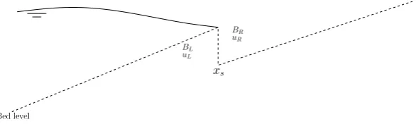
xs BR

uR

BL

uL

Bedlevel

Figure 3: Sketch of the shock forBat the shoreline in the physical domain

This method is found to be more stable than the approach of [18] and [10]. If bed friction is included (cd 6= 0), the shoreline may advance but never retreat in the physical domain [20]. Instead, a vanishingly thin film of water develops in the backwash, so the term −cd|u_h|u in (27) can become very large in this vicinity [21]. This can lead to numerical problems. Therefore we instead imposed h(x=L) =hmin in the backwash.

150

3.2.1. Shoreline boundary conditions for c and B

The shoreline boundary conditions require particular attention because the bed level must now be allowed to change, but the bed level lies outside the computational domain when that section of shore dries. For some bed load formulae, the bed-evolution at the shoreline is related to a shock condition [21] where the bed level on the left and on the right of the shoreline point are different. Therefore, our shoreline boundary

155

conditions must include shock conditions in order to effect that change, and these must be applied differently depending on whether the shore is being wetted or dried.

In (28), ash→0 at the shoreline, E/h→ ∞, thus, right hand side of (15) is undefined (→ ∞) unless

c → ceq(= u2) to maintain the stability of the model. So, we take the equilibrium state for suspended concentration, c = u2

s, at the shoreline [16]. Here we exclude the effect of downslope diffusion in the

160

boundary conditions. We use extrapolation when we incorporate this diffusion.

For some bed load sediment transport formulae, the bed-evolution at the shoreline is related to a shock condition [21] where the bed level on the left and on the right of the shoreline point are different. Consequently The shock at the advancing/retreating tip (see Fig. 3) can be defined in terms of bed-levels and velocities on the left-side (wet region) and right-side (dry region) of the shoreline: BL,uL andBR,uR.

165

Since the dry region is also included in bed shock relation forBat the shoreline, the solution ofB atx=L

can be related to that in the dry region. Following [13], the shock condition at the shoreline can be obtained by integrating across a physical region [x1, x2] such that

d dt

Z x2

x1

Bdx+ Z x2

x1

3σu2dx= Z x2

x1

M(c−u2)dx (35)

Assuming that x1 < L+xs < x2, and in the limit of x1 → L+xs and x2 → L+xs, and assuming

cs=ceq=u2s, and hR= 0, uR= 0,hL= 0 anduL=us. (35) becomes

170

−us[B]xx21+ [σu

3_]x2

x1= 0 (36)

⇒(BR−BL) +σu2s= 0 (37)

During uprush (us≥0), the dry bed levelBR is interpolated from known bed level at the previous time and the wet bed levelBLcan be obtained from (37). On the other hand, during backwash (us<0), the dry

175

bed level BR is unknown, and in this case, the bed level on left side BL is extrapolated linearly from the neighbouring nodes at the same time-step. Since the spatial grid size is small, the error of extrapolation is assumed negligible. OnceBL is known,BR is then computed from (37).

3.2.2. Offshore boundary condition

Here we adopt a characteristics-based boundary condition to allow waves to pass into and out of the

180

However, for simplicity, we here consider only (26)-(28). For the bed evolution (29), we use the original bed level with an assumption that the effects from nearshore area to the offshore boundary is so small as to be negligible, i.e. at offshore boundaryx= 0,B(0, t) = 0. The characteristic decomposition of (26)-(28) is

dR1

dt =−cd

|u|u

h −A2Bx on

dx

dt =A1+A2(u+

√

h) =λ1 (38)

185

dR2

dt =−cd

|u|u

h −A2Bx on

dx

dt =A1+A2(u−

√

h) =λ2 (39)

dR3

dt =

1

hE(u

2_{−c) on} dx

dt =u=λ3 (40)

where R1 = u+ 2 √

h, R2 = u−2 √

h and R3 = c. Thus, it can be seen that Riemann invariants are

unaffected by the transformation, whereas two of the characteristics are changed. The equation governing

190

R1 (R2) carries information in the positive (negative) direction, as long asλ1>0 (λ2<0).

In order to impose the boundary condition atx= 0 properly, we assume that at the offshore boundary

λ1<0 andλ2>0. Then the incoming signalR1 needs to be specified while the outgoing signalR2can be

determined from (39). Following [23],h(0, t) and u(0, t) can be computed by superimposing the incoming and outgoing waves at the boundary: h(0, t) = h(0,0) +ηi(0, t) +ηr(0, t) and u(0, t) = ui(0, t) +ur(0, t)

195

whereηis water surface elevation with respect to still water level. Subscriptsiandrindicate incoming and outgoing signals, respectively.

R2(0, tn+1) can be computed numerically from present and previous time levelstn,tn−1. If the incoming

waves is specified with knownηi,ηrcan be approximated by linear wave theory

ηr(0, t) =−

h(0,0) +R2(0, t)

p

h(0,0)

2 (41)

200

ui(0, t) =

ηi(0, t) p

h(0, t) (42)

ur(0, t) =−

ηr(0, t) p

h(0, t) (43)

Similarly, (40) is used to describe the offshore boundary condition for c(0, t). In this case, R3 carries

information along +xfor λ3 >0 and vice versa, along−xfor λ3 <0. Thus, foru(0, t)≥ 0, information 205

from outside the domain is required for specifyingR3. This can be done by extrapolation from the interior

domain, but instead here the instantaneous equilibrium state (neither erosion nor deposition) is assumed, i.e. c(0, t) =ceq =u(0, t)2. Ifu(0, t)<0, (40) is computed numerically from inside the domain to obtain

c(0, t).

4. Numerical solver

210

The equations (26)-(29) are solved numerically in the transformed computational domain. Note that the transformed equations include nonlinear termsA1(x, t) and A2(x, t). A finite difference scheme of spatial

derivatives in conjunction with an explicit time-stepping scheme are applied to solve for unknown variables. The computational domain is discretised intoN+ 2 nodes with node order fromj= 0 (offshore) toj =

N+ 1 (shoreline). The spatial derivatives are computed using fourth order central difference approximation

215

∂X ∂x

_j

= 1

12∆x

Xj−2−8Xj−1+ 8Xj+1−Xj+2

+O(∆x4) (44)

where ∆xis the distance between nodes, X represents any dependent variable andj is the spatial node at which the derivative is calculated, which is only valid fromj = 2 toj =N −1. At j = 1 andj =N, a second order central difference approximation is used. At the boundary node j = 0 and j =N + 1, the

220

Given initial conditions and boundary conditions, the modified NSWEs are integrated in time using an Adams-Bashforth-Moulton predictor-corrector scheme. The equations (26)-(29) can be written in the form

X_t=F (45)

A second order Adams-Bashforth scheme is applied for prediction, while a third order Adams-Moulton

225

scheme is used iteratively for correction of predicted variablesX at the next time-step.

X_Pn+1=Xn+∆t 2

h

3Fn−Fn−1i (46)

X_Cn+1=Xn+∆t 12 h

5F_Pn+1+ 8Fn−Fn−1i (47)

It is noted that an apparently non-physical oscillation occurs in this scheme and also in other schemes [24],

230

[9]. It appears to originate to the vicinity ofx=L. The cause of this behaviour is unknown but it is noted that [9] observed similar behaviour. Here we treat it in the same way as those authors by using a numerical filter technique developed by [24]. The filter is applied after every 100 time-steps to prevent spurious growth and avoid model instability. Moreover, the decentred Shapiro filter method developed by [25] also allows boundary filtering as well as centred filtering of the original Shapiro filter. For a computational domain of

235

N+ 2 nodes, nodesi= 4 toN−1 are filtered using the 16th_{-order Shapiro filter:}

F16(Xi) = 1 256

−(Xi−4+Xi+4) + 8(Xi−3+Xi+3)−28(Xi−2+Xi+2) + 56(Xi−1+Xi+1) + 186Xi

(48)

Near the boundaries, a non-symmetric filter is used as mentioned. Accordingly, at nodesi = 1,2,3, N − 2, N−1, N, the decentred 16th-order Shapiro filter is applied following [25].

5. Verification

240

5.1. Hydrodynamics only

We first consider hydrodynamics, equations (26) and (27), only. Analytical results were obtained by [26] for NSWEs on a plane beach of slope tanαby using a hodograph transformation methodology. There are two tests considered: transient and periodic. Both cases comprise useful verification tests for 1D hydrodynamic motion.

245

5.1.1. Carrier and Greenspan [1958] (CG58) transient solution

The transient case is the CG58 analytical solution for a body of fluid that is initially depressed (with respect to the still water level) and held motionless (u = 0) and then released at t = 0. The generated transient wave runs up the plane beach and allows us to see the model performance on the run-up problem. The case is transient, allowing us to ignore the offshore boundary by taking the domain far enough away

250

so that its influence can be neglected. The initial surface elevationη versusxis shown in Fig.4b and given analytically by CG58. They introduce a parameter ε related to depression of the initial surface elevation profile. A value of ε ≤ 0.23 needs to be selected for non-breaking cases. The initial surface elevation η

approaches asymptotically ε far offshore, and has a minimum value of 0 at the shoreline. The analytical solutions are obtained in (σ, λ)-coordinates (see formulas (3.4) - (3.9) in CG58). Hereinafter, we use χ to

255

denote the CG58σto avoid confusion with the present use ofσ. The motion of the instantaneous shoreline was obtained by settingχ= 0 (see formulas (3.10) - (3.13) in CG58).

The present model is tested against the transient case withL= 50, slope = 1/50, ∆x= 0.1, ∆t= 0.01,

α= 0.01,β = 0.024375, andε= 0.1. There are 500 nodes across the domain and the model are simulated over a time length of 100.

260

0 20 40 60 80 100

0 1 2 3 4 5 6

-0.1 0 0.1 0.2

(a)

15 20 25 30 35 40 45 50 55 60

0 0.02 0.04 0.06 0.08 0.1 0.12

(b)

Figure 4: Present results (solid line) against analytical CG58 transient solutions (square dotted) of (a): the shoreline position

xsand the shoreline velocityusversus timetand (b): the water surface elevationηversus cross-shore positionxat different time steps (t= 0−44 with ∆t= 4.4). The timet= 0 corresponds to the bottom line, and the top line corresponds tot= 44

5.1.2. CG58 periodic solution

CG58 also presented an analytical solution for periodic non-breaking standing waves on a plane-sloping beach, in which the periodic waves have amplitude A and frequency ω. This periodic behaviour can be

265

interpreted as a sinusoidal tide or non-breaking surface gravity wave in the swash. The periodicity of this wave allows us to verify the stability of the numerical model for very long times. The solution of this type of flow are specified by means of potential function: φ(χ, λ) =AJ0(ωχ) sin(ωλ), whereJ0is a zeroth order

Bessel function of the first kind. Once the values of Aand ω are defined, then the analytical solutions of flow properties can be solved for in the (χ, λ)-coordinates and converted back into (x, t) coordinates (see

270

formulas (2.16) - (2.19) in CG58) by solving a system of nonlinear equations usingfsolve in MATLAB. At the offshore boundary, the nonlinear system can also be solved numerically to obtain the analytical solution there. However, this is time consuming. Instead, a generating-absorbing boundary condition is used (see 3.2.2). A sinusoidal incoming signal is specified at the offshore boundary

ηi=

Hi 2 sin

2π

T t (49)

275

where Hi is incoming wave height, T is wave period. [27] and [28] pointed out that nonlinear effects are negligible far from the shoreline. Thus, the hydrodynamic variables far from the shoreline can be approximated in the uncoupled system of equations and the (χ, λ)-coordinates correspond directly to (x, t )-coordinates. To ensure that nonlinear effects are negligible, we must haveL >4 [27]. Also,Lis chosen such that the anti-node is formed at the offshore boundary. Following the simplification given in (2.10) of [28],

280

Acan be approximated by

A≈ 4Aof f

J0( √

16L) (50)

where Aof f is the amplitude of the signal at the offshore boundary. Since an anti-node is formed at the offshore boundary,Hi=Aof f.

Here we take slope = 0.1,Hi = 0.016,T = 10.0,L= 12.4, ∆x= 0.2, ∆t= 0.01,α= 0.01,β = 0.0983.

285

For given parameters, the corresponding CG58 analytical parameters obtained from above procedure are

A= 0.4, ω= 1. We have about 25 nodes over one wavelength, and about 890 timesteps per period.

are very small at the boundary. There is a small difference in the amplitude (0.2% relative error) which is

290

mainly due to the outgoing signal not perfectly exiting the domain.

0 0.5 1 1.5 2 2.5 3

-1 -0.5 0 0.5 1

-1 -0.5 0 0.5 1

(a)

0 0.5 1 1.5 2 2.5 3

-0.015 -0.01 -0.005 0 0.005 0.01 0.015

-0.015 -0.01 -0.005 0 0.005 0.01 0.015

(b)

Figure 5: Present results (solid line) against analytical CG58 periodic solutions (black squared) of (a): shoreline hydrodynamics

xsandusversus timet/T (b): offshore hydrodynamicsηof f anduof f versus timet/T

The shoreline positionxs and velocityus againstt/T are shown in Fig.5a. The maximum relative error between model and analytical solutions is about 0.5%. The agreement can also be observed in the evolution ofη anduover a full period (Fig. 6). There are small disagreements at the shoreline, which are similar to those observed in other models. These seem to result from phasing errors rather than numerical difficulties

295

because solutions are smooth in this vicinity. The stability of the model is also confirmed by running the model for about 100 periods whilst maintaining similar accuracy.

9 9.5 10 10.5 11 11.5 12 12.5

-1 -0.5 0 0.5 1

(a)

9 9.5 10 10.5 11 11.5 12 12.5

-0.6 -0.4 -0.2 0 0.2 0.4 0.6

(b)

5.1.3. Hubbard and Dodd [2002] model for periodic NSWEs

We now bring together periodic motion and bed friction, and verify against the NSWEs model of [29]. A sloping bed of domain lengthL= 12.4, slope = 0.1 was used for the simulation. The water level is still

300

initially,η(t= 0) = 0, u(t= 0) = 0 over the whole domain. For the present model, α= 0.01, β = 0.0983, ∆x= 0.1, ∆t= 0.01. The sinusoidal incoming signal isHi= 0.02,T = 10, andcd= 0,0.01,0.025 and 0.1. The model of [29] is a NSWEs model which include the alongshore component. The equations are solved in a fixed coordinate system. For both model an identical bathymetry, friction coefficients and driving signal are used. The domain length of 13.0 is used in [29] model, to allow the maximum run up to be included

305

within the domain. As presented above, a minimum water depthhmin = 10−5 is applied for both models. It is also noted that [29] also introduce a second depth tolerancehT OL to stabilise the scheme, which defines an ’almost dry’ cell [29]. For smooth solutions in [29] model, we use 1300 cells in the cross-shore direction. The Courant number = 0.8 andhT OL= 10×hminare used. The outgoing signal was not provided explicitly in [29] model but can be obtained easily from superposition assumption as the incoming and the summation

310

signals are known.

For the frictionless case,cd= 0, the total surface elevationη(x= 0) and depth-averaged velocityu(x= 0) at the offshore boundary are shown in Fig. 7a and 7b. The offshore signals of bothη anduare generally in good agreement with obvious disagreement only in troughs of the standing wave. Note that Fig. 7a and 7b show the initial generation of the wave and its subsequent complete reflection, with the comparison ofxs

315

forcd= 0 shown in Fig. 7c. The comparison between present and [29] solutions ofxs forcd= 0.01,0.025 and 0.1 are also shown in Fig. 7c. Overall agreement is not perfect, the solution obtained by the present model is smoother. It is noted that the spatial grid of the present model is 10 times larger than [29] for a similar degree of accuracy. This is mainly due to the transformation functions in (22) and (23) obtain a better resolution in the vicinity of the shoreline. Moreover, the second depth threshold is not required for

320

the present model, thus smoother solutions are obtained as can be seen in Fig. 7c.

5.2. Advection of suspended sediment in Shen and Meyer [1963] solution

[30] presented an analytical solution of the NSWEs corresponding to a bore impinging on a beach and subsequently running up and back down an initially dry slope. This swash motion was subsequently reinterpreted by [31] as an initial value problem. In general, the present model is developed for non-breaking

325

waves, but this solution can be accommodated. Only the initial condition contains a discontinuity and no shock subsequently develops. Although it could be argued that accurate modelling ofhanduensure accurate modelling ofc, becausecis passively advected at speedu, it is useful nonetheless as a verification case partly for reassurance and partly as a first step toward full morphodynamic coupling. To this end, we use the initial condition of [31], which in the physical domain is

330

u(x,0) = 0

c(x,0) = 0

for allx and

h(x,0) = 1.0 forx≤x0

h(x,0) = 0.0 forx > x0

(51)

The domain length extends far enough offshore so that the offshore boundary is not affected by the dam collapse throughout the simulation. OnceR2 at the boundary is known, then

R1=R2+ 4

p

h0 (52)

We takeL= 50, slope = 0.1, andα= 0.01,β = 0.024375. In this simulation, grid sizes of ∆x= 0.02 and

335

∆t = 0.001 are used. The exchange rate parameter E (see [17]) is chosen to be 0.001 and 0.03, which are consistent with the parameters used by [16]. The present results ofhanduare very close to the analytical solutions [31] (not shown).

The deviation ofcfrom its equilibrium value forE= 0.001 and 0.03 is shown as contour plots in Fig. 8a and 8b, respectively. The quantity ofc−ceq (orc−u2) is related to the tendency to erosion or deposition of

340

0 2 4 6 8 10 t/T

-0.8 -0.6 -0.4 -0.2 0 0.2 0.4 0.6 0.8

u

(

¯

x

=

0)

/H

i

(a)

0 2 4 6 8 10

t/T

-1 -0.8 -0.6 -0.4 -0.2 0 0.2 0.4 0.6 0.8

η

(

¯

x

=

0)

/H

i

(b)

5

5.5

6

6.5

7

-0.1

-0.05

0

0.05

0.1

(c)

Figure 7: Present (solid lines) and [29] (dashed lines) solutions of (a): the offshore water surface elevationηof f, (b): the offshore velocityuof f forcd= 0 and (c): the shoreline positionxsversustforcd= 0 (black), 0.01 (red), 0.025 (blue), 0.1(magenta)

5.3. Bed change due to bed load only over a single event

We now consider the same initial condition as for §5.2 but now an erodible bed is included, such that

σ >0 and M = 0. Therefore, although we allow suspended load transport to occur, bed change is only

345

affected by bed-load transport. Again, the same parameters and grid sizes ∆xand ∆t as used in 5.2 are applied. Here,σ= 0.01 is used so we can compare the results with [32].

The results of the beachface evolution are shown in Fig.9 with the final bed change shown in Fig.9b. Overall, the coupled simulation results agree well in comparison to [32] and [21] with similar patterns of hydrodynamics and bed-change.

350

5.4. Bed change due to bed load only over multiple periods

So far, the model performance has been confirmed through hydrodynamics, advection of sediment and bed change verification tests (see 5.1, 5.2 and 5.3). The latter two tests have been for a single event only. It is desirable to test over long duration if this approach is able to be used for long-term prediction. However, it is difficult to find benchmark results for long term simulations (i.e. either storm scale for wind

355

0 5 10 15 20 0

5 10 15 20 25 30 35 40

-1

-0.5

-0.1

-0.05 -0.01

0.01

0.05

0.1 0.2

0.01

-0.01 -0.05

-0.1

-0.5

-1

(a)

0 5 10 15 20

0 5 10 15 20 25 30 35 40

-0.1 -0.05 -0.01

-1

0 0.01 0.05 0.1

-0.1

-0.5

-1

-0.01 0

-0.05

(b)

Figure 8: Contour plots of present model solution (black) against [16] (red dashed) ofc−u2 _{for exchange rate parameter of} (a):E= 0.001 and (b): E= 0.03

(a)

0 5 10 15 20

-0.09 -0.08 -0.07 -0.06 -0.05 -0.04 -0.03 -0.02 -0.01 0 0.01

(b)

Figure 9: (a): Contour plots of ∆B, (b): Final bed change ∆Bfor [31] swash event over a mobile bed ofσ= 0.01 andM= 0 (present model: black solid line, [21]: red dashed line)

model includes bottom friction and the bed-load transport due to the Grass formula. It is noted that the Meyer-Peter-M´uller transportation equation applied in our model and the Grass formula are identical for

us,cr =ubcr= 0 (see 2). In this test, the bed diffusion with downslope mobilisation, i.e. (32) is considered

360

instead of (29).

It is noted that [33] reproduced the validation test for wind wave over storm-scale duration, showing a close agreement with results of [14]. Hence, we use the cross-shore results of [33] for impermeable bed and non-breaking incoming waves as a benchmark for verification. The physical parameter in [33] are set as follows: cd = 0.025, A= 0.004s2m−1, p= 0.4 and φ = 320, which are equivalent to σ= 0.0654 in the

365

present model.

4.5 5 5.5 6 6.5 7 7.5 8 -0.1

-0.05 0 0.05 0.1 0.15 0.2 0.25

(a)

0 800 1600 2400 3200 4000

-1.5 -1 -0.5 0 0.5

1 10 -6

(b)

Figure 10: (a): Bed change ∆B between present model (dashed line) and [33] model (solid line) at t = 1,000T (black),

t= 2,000T (red),t= 3,000T (blue) andt= 4,000T (magenta). (b)Sediment conservation of present model

proposed in [29]; a secondary thresholdhT OL is used, below which the velocity is considered to be zero (see [29] for more details). hmin = 0.002mandhT OL= 0.0025mare used. The initial bed bathymetry is given by [14]. In particular, the initial beach slope = tan 80, the still water depth at seaward boundaryh(x= 0) = 1

370

and the domain length is L= 7.115. The water is set to be still initially (t = 0). For the present model,

α= 0.01, β = 0.171, ∆x= 0.03 and ∆t = 0.002 are used. The number of spatial cells between the two models are consistent. The incoming signal is a series of sinusoidal waves with periodT = 5πandH= 0.025 (equivalent toT = 5sandH = 0.025min [14] model). The simulation duration is 4,000 periods. The same boundary condition as [33] is applied to obtain the hydrodynamics ((38) and (39) in 3.2.2). The bed level

375

at offshore boundary B(x = 0) is updated setting it equal to that at the next node at each time step, following the extrapolation approach proposed by [14]. The shoreline boundary condition are presented in 3.2 with the bed level is updated from previous time step. Fig. 10 shows the evolution of the bed profiles in comparison with [33]. The formation of a bar can be observed atx= 5.5 after 1000 periods in Fig. 10a. This bar develops and advances seaward, along with the erosive action in the upper part of the beach. Fig.

380

10a also shows a direct comparison of the bed change ∆B between the present model and [33]. Overall, the bed profiles between the two models are in good agreement with some discrepancy in the upper part of the beach. It is not clear what causes this small discrepancy. The secondary threshold in the model of [33] appears not to be responsible because a similar discrepancy is observed when it is removed.

The conservation of sediment in present model is also confirmed by checking the difference between the

385

net bed change and the net sediment transport at the offshore boundary due to bed load transport over time fromt= 0−Ti(Ti=iT withiis the number of periods, which range from 0 -4000 in this simulation). Fig. 10b shows that the difference between these two values over simulation duration is very small in the order of 10−6, which confirm the conservation of sediment in present model.

6. Conclusions

390

A morphodynamical model for NSWEs plus sediment advection and bed-evolution equations have been developed for long, non-breaking waves. The model involves a predictor-corrector time integration in con-junction with finite difference for approximation of spatial derivatives. The performances of the present model are confirmed against both hydrodynamic and morphodynamic. The morphodynamical performances of present model are also validated against known models for a single swash event and mid-term simulations.

395

in morphodynamical results. However, the difference are small while the conservation of sediment is still maintained.

In conclusion, good agreement in present model in storm scale tests also suggests that the model is suitable for further study of long-term morphodynamic of long waves such as tides and non-breaking wind

400

waves. The model can also be extended into 2DH to include alongshore factors. It confirm that coordinate transformation techniques can also be used to accurately simulate short and long-term morphodynamic changes.

Acknowledgements

This research is sponsored by Faculty of Engineering, The University of Nottingham, UK. The authors

405

would like to thank Riccardo Briganti and Giorgio Incelli, of University of Nottingham, for providing the results of mid-term (storm scale) test.

References

[1] C. C. Mei, The applied dynamics of ocean surface waves, 1st Edition, Vol. 1 of Advanced Series on Ocean Engineering, World Scientific, 1989.

410

[2] M. Brocchini, N. Dodd, Nonlinear shallow water equation modelling for coastal engineering, Journal of Waterway, Port, Coastal and Ocean Engineering 134 (2) (2008) 104–120.

[3] S. Hibberd, D. Peregrine, Surf and run-up on a beach: a uniform bore, Journal of Fluid Mechanics 95 (2) (1979) 323–345. [4] P. F. Liu, Y. S. Cho, M. Briggs, U. Lu, C. Synolakis, Runup of solitary waves on a circular island, Journal of Fluid

Mechanics 302 (1995) 259–285. 415

[5] P. J. Lynett, T. R. Wu, P. F. Liu, Modeling wave runup with depth-integrated equations, Coastal Engineering 46 (2002) 89–107.

[6] A. V. Dongeren, I. Svendsen, An absorbing-generating boundary condition for shallow water models, Journal of Waterway, Port, Coastal and Ocean Engineering 123 (6) (1997) 303–313.

[7] B. Johns, Numerical integration of the shallow water equations over a sloping shelf, International Journal for Numerical 420

Methods in Fluids 2 (1982) 253–261.

[8] H. Takeda, Numerical simulation of run-up by variable transformation, Journal of The Oceanographical Society of Japan 40 (1984) 271–278.

[9] H. T. ¨Ozkan-Haller, J. T. Kirby, A Fourier-Chebyshev collocation method for the shallow water equations including shoreline runup, Applied Ocean Research 19 (1997) 21–34.

425

[10] R. Prasad, I. Svendsen, Moving shoreline boundary condition for nearshore models, Coastal Engineering 49 (2003) 239–261. [11] F. Ribas, A. Falqu´es, H. E. de Swart, N. Dodd, R. Garnier, D. Calvete, Understading coastal morphodynamic patterns

from depth-averaged sediment concentration, Reviews of Geophysics 53 (2) (2015) 362–410. [12] R. L. Soulsby, Dynamics of marine sands, 1st Edition, Thomas Telford, 1997.

[13] D. M. Kelly, N. Dodd, Beach face evolution in the swash zone, Journal of Fluid Mechanics 661 (2010) 316–340. 430

[14] N. Dodd, A. M. Stoker, D. Calvete, A. Sriariyawat, On beach cusp formation, Journal of Fluid Mechanics 597 (2008) 145–169.

[15] D. Pritchard, A. J. Hogg, On fine sediment transport by long waves in the swash zone of a plane beach, Journal of Fluid Mechanics 493 (2003) 255–275.

[16] F. Zhu, N. Dodd, The morphodynamics of a swash event on an erodible beach, Journal of Fluid Mechanics 762 (2015) 435

110–140.

[17] D. Pritchard, A. J. Hogg, On the transport of suspended sediment by a swash event on a plane beach, Coastal Engineering 52 (2005) 1–23.

[18] M. Brocchini, I. Svendsen, R. Prasad, G. Bellotti, A comparison of two different types of shoreline boundary conditions, Computer methods in applied mechanics and engineering 1991 (2002) 4475–4496.

440

[19] R. J. Sobey, Wetting and drying in coastal flows, Coastal Engineering 56 (2009) 565–576.

[20] M. Antuono, L. Soldini, M. Brocchini, On the role of the chezy frictional term near the shoreline, Theoretical and Computational Fluid Dynamics 26 (2012) 105–116.

[21] F. Zhu, N. Dodd, Net beach change in the swash zone: A numerical investigation, Advances in Water Resources 53 (2013) 12–22.

445

[22] G. Incelli, R. Briganti, N. Dodd, Absorbing-generating seaward boundary conditions for fully-coupled hydro-morphodynamical solvers, Coastal Engineering 99 (2015) 96–108.

[23] N. Kobayashi, A. K. Otta, I. Roy, Wave reflection and runup on rough slopes, Journal of Waterway, Port, Coastal and Ocean Engineering 113 (3) (1987) 282–298.

[24] R. Shapiro, Smoothing, filtering and boundary effects, Review of Geophysics and Space Physics 8 (2) (1970) 359–387. 450

[26] G. Carrier, H. Greenspan, Water waves of finite amplitude on a sloping beach, Journal of Fluid Mechanics 1 (4) (1958) 97–109.

[27] G. Carrier, Gravity waves on water of variable depth, Journal of Fluid Mechanics 24 (4) (1966) 641–659. 455

[28] C. Synolakis, The runup of solitary waves, Journal of Fluid Mechanics 185 (1987) 523–545.

[29] M. E. Hubbard, N. Dodd, A 2d numerical model of wave runup and overtopping, Coastal Engineering 47 (2002) 1–26. [30] M. C. Shen, R. E. Meyer, Climb of a bore on a beach. part 3: Run-up, Journal of Fluid Mechanics 16 (1) (1963) 113–125. [31] D. H. Peregrine, S. M. Williams, Swash overtopping a truncated plane beach, Journal of Fluid Mechanics 440 (2001)

391–399. 460

[32] F. Zhu, 1d morphodynamical modelling of swash zone beachface evolution, Ph.D. thesis, University of Nottingham (2012). [33] G. Incelli, A fully-coupled coastal hydro-morphodynamical numerical solver, Ph.D. thesis, University of Nottingham