A novel model for Uncertainty Propagation analysis
applied for human thermal comfort evaluation
ANDREA MANUELLO BERTETTO
Department of Ingegneria Meccanica, Chimica e dei Materiali
Università degli Studi di Cagliari
Via Marengo 2, 09123 Cagliari
ITALY
[email protected]
LUIGI ANTONIO BESALDUCH
Department of Ingegneria Civile Ambientale e Architettura
Università degli Studi di Cagliari
Via Marengo 2, 09123 Cagliari
ITALY
[email protected]
EDMONDO MINISCI
Department of Mechanical and Aerospace Engineering
University of Strathclyde
G1 1XQGlasgow UK
[email protected]
MARTIN KUBICEK
Department of Mechanical and Aerospace Engineering
University of Strathclyde
G1 1XQ Glasgow UK
[email protected]
ROBERTO RICCIU
Dipartimento di Ingegneria Civile Ambientale e Architettura
Università degli Studi di Cagliari
Via Marengo 2, 09123 Cagliari
ITALY
[email protected]
Abstract: The comfort sensation is mainly affected by six variables: air temperature,
mean radiant temperature, air velocity, relative humidity, personal metabolism and clothing insulation. These are characterized by different mean values and distributions.
To analyze the uncertainty propagation three numerical models are used: the Fully Monte Carlo Simulation MCSs, the Monte Carlo Simulation Trials MCSt, and a novel model named "Adaptive Derivative based High Dimensional Model Representation" (AD-HDMR). In the paper these three different methods are applied to the thermal comfort evaluation, through the PMV Index, they are analyzed and their efficiency was verified in terms of computational time. To allow a revision of this index, the effect of the different variables was then analyzed.
Key-Words: Mathematical models, Statistical analysis, Thermal comfort, Engineering
1 Introduction
The steady growth of the performance of modern computers, accompanied by a gradual decrease of the associated costs, has been encouraging the numerical simulation of more complex physical problems.
The most general way to perform uncertainty propagation (UP), as well as global sensitivity analysis, is to use the Monte-Carlo (MC) approach, which basically follows three main steps:
1) sample the input random variable(s) from their known or assumed (joint) Probability Density Function (PDF),
2) compute deterministic output for each sampled input value(s), and
3) determine the statistical characteristics of the output distribution (e.g. mean, variance, skewness). The MC method has the property that it converges to the exact stochastic solution when the number of samples n→∞. In practice the value of n can be a finite number, but to have a highly converged process it should be very high, causing an excessive computational costs (even for modern computers). A way to reduce the computational time of the UP process could be to build a less expensive surrogate of the model and then use it to propagate the uncertainty. Among the surrogate based approaches, there are the Stochastic Collocation (SC) method, the Polynomial Chaos (PC) [1], and the Kriging surrogate model [2]. These methods are non-intrusive by nature, because they consider the model as a black box and try to approximate the implemented function. One of the major issues of the surrogate based approaches is the so called Curse of Dimensionality (CoD) [3], which limits their use to problems with low dimensionality. The cut-High Dimensional Model Representation (cut-HDMR) [4] was developed to decouple the interaction effects of chemical systems, and was successfully used in other fields such as uncertainty quantification [5], sensitivity analysis [6] and interpolation problems [7].
In this work a new method for UP is used and compared to the results given by MC. The used approach decomposes the stochastic space into sub-domains, which are then interpolated separately by a selected interpolation technique [8]. Each interpolating model is built accordingly to the outcomes of a new derivation of the cut-HDMR. The contribution of each independent sub-domain to the final response is evaluated, and only important sub-domains are sampled and interpolated, causing a dramatically reduction of the necessary number of samples for high dimensional spaces.
The MC simulation is then applied on each important interpolated sub-domain to approximate the propagation of uncertainty, as well as the sensitivity of the global function w.r.t. the single variables or combinations of variables. The specific application in this work is implemented in human comfort topic.
The thermal comfort in indoor environment play an important role, but often neglected, in the design of new buildings, or in the renovation of old ones. In particular in residential buildings, where designing only considering energy saving aspects could cause overheated or overcooled indoor climate condition [9], or in educational buildings, where it could cause loss of attention and learning ability problems, and if protract even asthmatic symptoms [10, 11].
In 1970 Fanger [12] introduced a method to predict the level of thermos-hygrometric comfort within a confined space as happens in residential buildings. The UNI EN ISO 7730 [13] takes up this theory. Through the measurement of four physical quantities (air velocity, air temperature, radiant temperature and relative humidity) and two subjective (clothing and personal metabolism) by applying the mathematical relationship contained in this standard, it is possible to reach statistical index called Predicted Mean Vote (PMV index). Through a 7-point scale (Table 1) in which a score is associated with the thermal sensation of the human body [12, 13,14].
Table 1: Thermal sensation scale in ISO 7730:05
+3 Hot
+2 Warm
+1 Slightly warm
0 Neutral
-1 Slightly cool -2 Cool
-3 Cold
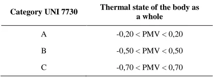
[image:2.595.323.532.676.752.2]The same ISO 7730 provides a further subdivision of the value of the PMV shown in Table 2.
Table 2: ISO 7730:05 in PMV Classification
Category UNI 7730 Thermal state of the body as a whole
A -0,20 < PMV < 0,20
B -0,50 < PMV < 0,50
The characteristics of the measures in situ by the four mechanical parameters are imposed by the standard UNI EN ISO 7726 [15] such as field and uncertainty about the nature of physical measurements follow a Gaussian distribution. The characteristics of the measures for the two sizes are imposed by subjective standards: the UNI EN ISO 8996 [16] takes into account the evaluation and measurement of human metabolism.
The UNI EN ISO 9920 [17] shows how to evaluate the thermal resistance of clothing through direct and indirect measures.
Olesen and others [18] associated with this evaluation an uncertainty distribution.
Some authors [19, 20, 21] have made the problem of verifying if starting from the uncertainties of the input variables to the system, which was the uncertainty of the PMV output.
Focus of this work is to apply the three numerical methods (fully Monte Carlo, Monte Carlo trials and the Derivative-HDRR) from common data, and to compare the results obtained and the computational costs.
2 The PMV Index
To evaluate the PMV, the model is established by UNI 13005 [12] and it is expressed by relation:
(
)
( ) [ ( ) ] ( ) [ ] ( ) ( ) ( )(
)
( ) − ⋅ − − + − + ⋅ ⋅ ⋅ − − − ⋅ − − − ⋅ ⋅ ⋅ − − − ⋅ − − − − ⋅ − ⋅ ⋅ − − ⋅ + ⋅ = − − − − a cl c cl r cl cl a a a M t t h f t t f t M p M W M p W M W M e PMV 4 4 8 5 3 036 . 0 273 273 10 96 . 3 34 4 001 . 0 5867 10 7 . 1 15 . 58 42 . 0 99 . 6 5733 10 05 . 3 028 . 0 303 . 0 (1) Where:( ) cl
{
cl[
(cl )(
r)
]
cl c(cl a)}
cl M W I f t t f h t t
t = − ⋅ − − ⋅ −8⋅ ⋅ + 4− + 4+ ⋅ −
273 273 10 96 . 3 028 . 0 7 . 35 ( ) ⋅ − = ar a cl c v t t h 1 . 12 38 .
2 0.25
for
for ( )
(cl a) ar
ar a cl v t t v t t 1 . 12 38 . 2 1 . 12 38 . 2 25 . 0 25 . 0 < − ⋅ > − ⋅ ⋅ + ⋅ + = cl cl cl I I f 645 . 0 05 . 1 290 . 1 00 . 1 for for W C m I W C m I cl cl / 078 . 0 / 078 . 0 2 2 ° ⋅ > ° ⋅ ≤
where the symbols are the same as in the table 3.
3 The simulation methods
A classical method to evaluate the uncertainties in the indirect measure is the Monte Carlo (MC), and
in fact the UNI 13005 [22] prescribes to use this method to assess the uncertainties of indirect measures.
As stated in the introduction, since the MC approach can be very computationally expensive, other approximated methods can be preferred. In this paper we use one of the alternative approaches, which is based on the cut-High Dimensional Model Representation (cut-HDMR) decomposition [23]. This technique decomposes the stochastic space into sub-domains of lower dimensionality, and interpolates each sub-domain with the most appropriate technique. It determines the range of coverage with the approximation degree of 95%, which is a measure of the model fidelity and of the information quality on the independent variables, contained in the probability density function. The instrumental accuracy required by the UNI EN ISO 7726 [15] was taken as the uncertainty of the physical variables. For the uncertainties associated with the variables M and Icl, reference was made to Olesen and others [18] and therefore, an associated uncertainty with rectangular distribution, and having the mean value equal to 15%, is assumed.
As regards the numerical methodology the Monte Carlo Methods “full” and “adaptive” according to the law are both applicable.
The main difference between them is that in the adaptive method the loop described in Figure 1 can be stopped when the variation of the statistical values with the iterations:
abs(f(x)nc-f(x)nc-100)
nc is the current number of samples, and is < 1e-5 ,
bringing to an n << 106. The full Monte Carlo is interrupted when N = 106, with N, nc are natural
numbers.
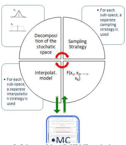
In Figure 1 the block diagram of the Monte Carlo Simulation is represented. In order to let the reader understand the difference between the MC approaches and the approximate one, the AD-HDMR (Adaptive Derivative High Dimensional Model Representation) method is briefly described in what follows.
stochastic variable and each one of their interactions through the model, considered as increments with the respect the nominal response, fc:
∑ ∑
[image:4.595.321.535.77.323.2]where n is the number of variables.
Figure 1: Block diagram of Monte Carlo Method.
A surrogate model representation can be independently generated for each element of the sum (called “Increment Functions”) and only for the non-zero elements, thus greatly reducing the complexity of sampling and building the model. Moreover, the contribution of each term of the sum to the global response can be quantified independently so that higher order interactions with low or zero contribution can be neglected already by analyzing the lower order terms.
of their interactions through the model, considered as increments with
[image:4.595.64.285.164.586.2]⋯ … (2)
Figure 1: Block diagram of Monte Carlo Method.
A surrogate model representation can be independently generated for each element of the (called “Increment Functions”) and only for the zero elements, thus greatly reducing the complexity of sampling and building the model. Moreover, the contribution of each term of the sum to the global response can be quantified igher order interactions with low or zero contribution can be neglected already by
Figure 2: Scheme of the AD
This particular approach can be used to propagate any known standard distribution, from the clas Gaussian and uniform, to Gumbell and Landau ones.
Not only is the output of this method the (multi dimensional) distribution of the quantity of interest, but also the quantification of the global contribution of each term of the sum to the global respo
feature, allows for a complete analysis of the sensitivity of the response with respect to each of the stochastic variables, as well as their interactions. Moreover in the case that the objective function should be considered as a black box, the
the single contributions can give an insight into the structure of the response function.
The selection of the important stochastic domains is done in two phases, the first phase predicts the importance of each
sub-second phase neglects the sub
little importance on the interpolation process. The prediction approach compares the importance of each stochastic variable and predicts the importance of its combination, i.e. interaction. The non important interactions of variables are then neglected and the adaptive sampling interpolation process starts.
The adaptive approach is based on an adaptive sampling technique, which compares the interpolation process in each iterative step. The position of a new sample is th
difference between these two interpolations, where the difference is computed as the change of a shape of the selected interpolation technique. The selected Figure 2: Scheme of the AD-HDMR method.
This particular approach can be used to propagate any known standard distribution, from the classic Gaussian and uniform, to Gumbell and Landau
Not only is the output of this method the (multi-dimensional) distribution of the quantity of interest, but also the quantification of the global contribution of each term of the sum to the global response. This feature, allows for a complete analysis of the sensitivity of the response with respect to each of the stochastic variables, as well as their interactions. Moreover in the case that the objective function should be considered as a black box, the analysis of the single contributions can give an insight into the structure of the response function.
The selection of the important stochastic domains is done in two phases, the first phase predicts the -design domain and the phase neglects the sub-design domains with little importance on the interpolation process. The prediction approach compares the importance of each stochastic variable and predicts the importance of its combination, i.e. interaction. The
non-actions of variables are then the adaptive sampling interpolation
interpolation technique is the so called Multi-surrogate adaptive technique, which is able to combine and exploit various interpolation techniques. The convergence process of the adaptive part is based on the observation of the statistical properties of the weight function propagated through the interpolation technique. Being the weight function the input distribution in the case of the UQ propagation, the change of the expected value and the standard deviation of the weight function assures that the model is accurate around the area of interest.
The Multi-surrogate Adaptive interpolation technique is particularly suited when the behavior of the underlying function is unknown a priori. In this case, it is very difficult, or impossible, to say which
one of the several available
interpolation/approximation technique should or could be used, and the Multi-surrogate Adaptive method is able to select the best interpolation techniques for the given problem, based on the
features of the function. The
interpolation/approximation techniques already implemented include polynomials, RBF, kriging and splines.
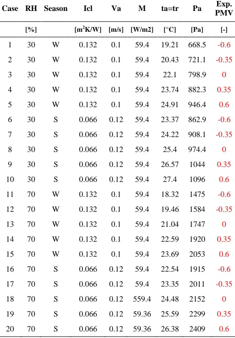
[image:5.595.310.546.149.488.2] [image:5.595.51.291.554.728.2]The three methods are implemented for 20 cases in Table 4, according to the values of the uncertainties and the distribution function of the individual input variables (Table 3) determined following the ENV 13005:1999.
Table 3: Metrological Characteristics of The input Variables and Corresponding Distribution Type
ISO 7730:05 in PMV Classification
Microclimate and subjective variables with uncertainty and corresponding distribution
Parameter
Symbols (units)
Standard
Deviation Distribution
Metabolic rate M (W/m2) ±15% Rectangular
Static clothing insulation
Icl (m2K/W) ±15% Rectangular
Vapour partial
pressure Pa (Pa) ±300 Pa Gaussian
Average radiant temperature
tr (°C) ±4°C Gaussian
Air temperature ta (°C) ±1°C Gaussian
Absolute air velocity
Va (m/s) 2*(0,05+
0,05Va) Gaussian
Table 4: 20 cases of simulation. The expected PMV value, calculated through the equation (1), in red
color . “w” and “s” indicate the two weather combination (winter and summer respectively), and
RH the relative humidity.
Case RH Season Icl Va M ta=tr Pa Exp.
PMV
[%] [m2K/W] [m/s] [W/m2] [°C] [Pa] [-]
1 30 W 0.132 0.1 59.4 19.21 668.5 -0.6
2 30 W 0.132 0.1 59.4 20.43 721.1 -0.35
3 30 W 0.132 0.1 59.4 22.1 798.9 0
4 30 W 0.132 0.1 59.4 23.74 882.3 0.35
5 30 W 0.132 0.1 59.4 24.91 946.4 0.6
6 30 S 0.066 0.12 59.4 23.37 862.9 -0.6
7 30 S 0.066 0.12 59.4 24.22 908.1 -0.35
8 30 S 0.066 0.12 59.4 25.4 974.4 0
9 30 S 0.066 0.12 59.4 26.57 1044 0.35
10 30 S 0.066 0.12 59.4 27.4 1096 0.6
11 70 W 0.132 0.1 59.4 18.32 1475 -0.6
12 70 W 0.132 0.1 59.4 19.46 1584 -0.35
13 70 W 0.132 0.1 59.4 21.04 1747 0
14 70 W 0.132 0.1 59.4 22.59 1920 0.35
15 70 W 0.132 0.1 59.4 23.69 2053 0.6
16 70 S 0.066 0.12 59.4 22.54 1915 -0.6
17 70 S 0.066 0.12 59.4 23.35 2011 -0.35
18 70 S 0.066 0.12 559.4 24.48 2152 0
19 70 S 0.066 0.12 59.36 25.59 2299 0.35
20 70 S 0.066 0.12 59.36 26.38 2409 0.6
4 Results
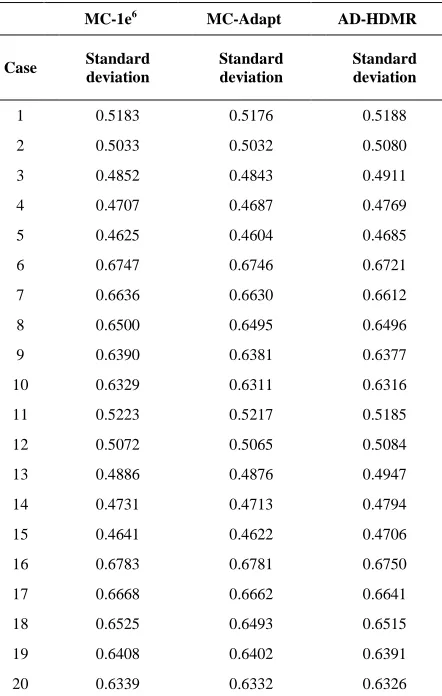
Table 5: Standard deviation of the 20 cases of simulation.MC-1e6 is the fully MonteCarlo method,
MC-Adapt is the adaptive MonteCarlo and AD-HDMR the Adaptive Derivative High Dimensional
Model Representation.
MC-1e6 MC-Adapt AD-HDMR
Case Standard deviation
Standard deviation
Standard deviation
1 0.5183 0.5176 0.5188
2 0.5033 0.5032 0.5080
3 0.4852 0.4843 0.4911
4 0.4707 0.4687 0.4769
5 0.4625 0.4604 0.4685
6 0.6747 0.6746 0.6721
7 0.6636 0.6630 0.6612
8 0.6500 0.6495 0.6496
9 0.6390 0.6381 0.6377
10 0.6329 0.6311 0.6316
11 0.5223 0.5217 0.5185
12 0.5072 0.5065 0.5084
13 0.4886 0.4876 0.4947
14 0.4731 0.4713 0.4794
15 0.4641 0.4622 0.4706
16 0.6783 0.6781 0.6750
17 0.6668 0.6662 0.6641
18 0.6525 0.6493 0.6515
19 0.6408 0.6402 0.6391
[image:6.595.57.278.142.490.2]20 0.6339 0.6332 0.6326
Table 6: Number of calls of the three methods for the 20 cases.
Case MC-1e6 MC-Adapt AD-HDMR
1 1E+06 33800 75
2 1E+06 43900 74
3 1E+06 34200 72
4 1E+06 17000 74
5 1E+06 17000 74
6 1E+06 48800 73
7 1E+06 12000 74
8 1E+06 44300 80
9 1E+06 39700 74
10 1E+06 32600 74
11 1E+06 33800 76
12 1E+06 33800 75
13 1E+06 33800 81
14 1E+06 17000 74
15 1E+06 17000 74
16 1E+06 48800 73
17 1E+06 12000 74
18 1E+06 15200 80
19 1E+06 44300 74
20 1E+06 44300 71
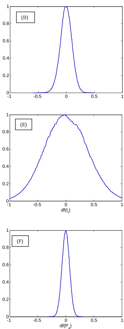
In the figure 3 the distribution of the increment function for the six different variables is shown. This quantity is relevant because is related to the importance of the variables in the variation of the PMV, and in particular wider is the curve, more important is the variable. In particular the random variable tr has the biggest influence on the final input
in terms of uncertainty. Its high variance means that this variable creates the largest uncertainty on the final output. The partial mean of this variable is negligible, meaning that this variable brings only uncertainty into the final output and an increase in accuracy of the input (decrease of the input uncertainty) does not influence the final expected value. The curve confirms that the input distribution is a Gaussian one and the underlying function is mainly linear. Instead the random variable Va has a
small influence on the final uncertainty and its influence on the final uncertainty is negligible. Decrease in the input uncertainty would not affect the final uncertainty. On the other hand, the partial mean has a large influence on the global mean. The shape of the curve show that the underlying function has high steep gradient around the central point and flat region close to it. This suggests that near the central point there is a discontinuity (due to the non significant negative velocity values). Moreover, due to a small number of samples on the right side of the figure, the curve confirms that the input distribution is Gaussian. This random variable can be used to increase or decrease the final expected value.
[image:6.595.46.284.551.765.2]Figure 3: Distribution of the increment function for the variables: (A) Static clothing insulation, (B) Absolute Air Velocity, (C) Metabolic Rate. The ordinate value is the number of sample normalized
[image:7.595.72.280.85.612.2]for the maximum value.
Figure 4: Distribution of the increment function for the variables: (D) Air temperature, (E) Average radiant temperature, (F) Vapor partial pressure. The
ordinate value is the number of sample normalized for the maximum value.
-1 -0.5 0 0.5 1
0.65 0.7 0.75 0.8 0.85 0.9 0.95 1
df(I )
-1 -0.5 0 0.5 1
0 0.2 0.4 0.6 0.8 1
df(Va)
-1 -0.5 0 0.5 1
0.4 0.5 0.6 0.7 0.8 0.9 1
df(M)
-1 -0.5 0 0.5 1
0 0.2 0.4 0.6 0.8 1
df(t )
-1 -0.5 0 0.5 1
0 0.2 0.4 0.6 0.8 1
df(tr)
-1 -0.5 0 0.5 1
0 0.2 0.4 0.6 0.8 1
df(Pa)
(A)
(B)
(C) (F)
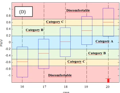
As shown in the figure 4, this behavior is more relevant in summer than in winter, and it is less affected by the relative humidity. The PMV model is consequently to restrictive for professional use and need a revision.
Figure 4: Boxplot of 20 the cases. (A) Cases from 1 to 5 with RH = 30% and winter season (B) Cases from 6 to 10 with RH = 30% and summer season (C)
Cases from 11 to 15 with RH = 60% and winter season (D) Cases from 16 to 20 with RH = 60% and
summer season.
4 Conclusion
In the final evaluation of the uncertainty of a
function dependent on several variables, the
Monte Carlo method is one of the two methods
proposed in the UNI ENV 13005. In particular,
this method, unlike other methods, allows to
simulate the variation of all the function
independent variables through their mean value,
its uncertainty and its distribution whatever the
mathematical model used. This leads to the
knowledge of the same parameters of the
unknown
variable
and
can
do
best
considerations on the results. Also a new
method
named
Adaptive Derivative HighDimensional Model Representation was compared with the other two to perform uncertainty propagation,
These models are applied to the computation of
the PMV index under 20 different cases, the
results are quite similar in all the simulation
condition, but comparing the computational
costs if the adaptive MonteCarlo simulation id
10
2times faster than the fully MonteCarlo
model, and the HDMR even more (10
4times).
Another important consideration can be done
analyzing the PMV statistical distribution, the
classification according to the ISO 7730:05 is
too restrictive for professional use, and the
comfort prediction is strongly affected by the
accuracy of the input variables so a revision of
this classification is desirable, in particular the
(A)
(B)
(C)
estimation of the PMV is strongly affected by
the radiant temperature, an higher precision in
the
estimation
of
this
parameter
is
recommended.
References:
[1] Eldred, M. Burkardt, J., Comparison of non-intrusive polynomial chaos and stochastic collocation methods for uncertainty quantification, In 47th AIAA Aerospace Sciences Meeting including The New Horizons Forum and Aerospace Exposition, Orlando, Florida, January 2009.
[2] Fang, K. T., Li, R., Sudjianto, A., Design and Modeling for Computer Experiments, Chapman and Hall/CRC press, New York, 2006.
[3] Bellman, R. E., Adaptive Control Processes: A Guided Tour, Princeton University Press, New Jersey, NJ, 1961
[4] Shorter, J. A., Ip, P. C., Rabitz, H. A., An efficient chemical kinetics solver using high dimensional model representation, J. Phys. Chem., 103:7192–7198, 1999.
[5] Lia, G., Wanga, S. W., Rabitza, H., Wangb, S., and Peter, Global uncertainty assessments by high dimensional model representations (hdmr), Chemical Engineering Science, 57, 2002.
[6] Li, G., Artamonov, M., Rabitz, H.,Wang, S.W., Georgopoulos, P. G., and Demiralp, M., High-dimensional model representations generated from low order termslp-rs-hdmr, Journal of Computational Chemistry, 24(5), 2003.
[7] Tunga, M. A., An approximation method to model multivariate interpolation problems: Indexing hdmr, Mathematical and Computer Modelling, 53:1970–1982, 2011.
[8] Kubicek, M., Minisci, E., Cisternino, M., High dimensional sensitivity analysis using surrogate modeling and High Dimensional Model Representation, to appear in “International Journal for Uncertainty Quantification”
[9] Jitka Mohelnikova Hasim Altan, Evaluation of Optical and Thermal Properties of Window Glazing, WSEAS TRANSACTIONS on
ENVIRONMENT and DEVELOPMENT,
Issue 1, Volume 5, January 2009
[10] Eusébio. Z. E. Conceicao, M. Manuela, J. R. Lùcio Margarida. C. Lopes, Application of an Indoor Greenhouse in the Energy and Thermal Comfort Performance in a Kindergarten School
Building in the South of Portugal in Winter Conditions, WSEAS TRANSACTIONS on ENVIRONMENT and DEVELOPMENT, issue 8, Volume 4, August 2008
[11] Teet-Andrus Koiv, Alo Mikola, Ulli-Kaisa Karro, The indoor climate and energy consumption of educational buildings, WSEAS TRANSACTIONS on ENVIRONMENT and DEVELOPMENT, Volume 10, 2014
[12] P.O., Fanger, Thermal Comfort-Analysis and Applications in Environmental Engineering, Copenhagen: Danish Technical Press, 1970. [13] EN ISO 7730:2005, Ergonomics of the thermal
environment - Analytical determination and interpretation of thermal comfort using calculation of the PMV and PPD indices and local thermal comfort criteria (ISO 7730:2005). [14] ASHRAE Standard 55-2013, Thermal Environmental Conditions for Human Occupancy
[15] EN ISO 7726:2001, Ergonomics of the thermal environment - Instruments for measuring physical quantities (ISO 7726:1998)
[16] EN ISO 8996:2004, Ergonomics of the thermal environment - Determination of metabolic rate (ISO 8996:2004)
[17] EN ISO 9920:2009, Ergonomics of the thermal environment - Estimation of thermal insulation and water vapor resistance of a clothing ensemble (ISO 9920:2007, Corrected version 2008-11-01
[18] Olesen, B.W., Parsons K.C., Introduction to thermal comfort standards and to the proposed new version of EN ISO 7730, Energy and Buildings, 34, 2002, 537-548.
[19] D'Ambrosio Alfano, F. R., Palella, B. I., Riccio, G., The role of measurement accuracy on the thermal environment assessment by means of PMV index, Building and Environment 46, 2011, pp. 1361–1369.
[20] Bertetto, A.M., Cadeddu, A., Niccolini, G., Di Pilla, L., Ricciu, R.
,
Home automation systems and PMV classification for moderate confined environments, 23rd International Conference on Robotics in Alpe-Adria-Danube Region, IEEE RAAD 2014 - Conference Proceedings 7002277[21] Ricciu, R., Desogus, G., Mura, S., Thermal comfort analysis by the PMV index. Applying the Monte Carlo simulation for evaluating the probability distribution, AICAAR congress: Baveno 2012
[23] Hooker, G., Discovering additive structure in black box functions, In KDD 04 Proceedings of the tenth ACM SIGKDD international conference on Knowledge discovery and data mining, pp. 575–580. ACM New York, NY, USA, 2004.
[24] Gozen Guner Aktas, Design Parameters and Initiatives for Ecological and Green Design in
Interior Architecture, WSEAS