The fin blue line : quantifying fishing mortality using shark fin morphology

(1)

The Fin Blue Line

Quantifying Fishing Mortality Using Shark Fin

Morphology

Lindsay Marshall

Bachelor of Marine Science (Honours) Murdoch University

Submitted in fulfilment of the requirements for the Degree of Doctor of Philosophy

University of Tasmania April 2011

Supervisors Dr Alistair Hobday

(2)

Declaration of Originality

This thesis contains no material which has been accepted for a degree or diploma by the University or any other institution, except by way of background information and duly acknowledged in the thesis, and to the best of the my knowledge and belief no material previously published or written by another person except where due acknowledgement is made in the text of the thesis, nor does the thesis contain any material that infringes copyright.

Lindsay Marshall

Statement of Access

This thesis may be made available for loan and limited copying in accordance with the Copyright Act 1968.

(3)

Abstract

Overfishing is a major global concern. Many of the worlds fish stocks are currently over exploited and require immediate action toward effective management and recovery strategies. Sharks are especially susceptible to overexploitation as they are generally slow growing, late maturing and produce few young. As large predators, sharks play an important, but poorly understood, role in marine food webs. As such, the ongoing exploitation of shark stocks is likely to cause detrimental and lasting ecological shifts within many marine systems.

Within numerous fisheries, sharks are primarily targeted for their highly priced fins, and in many cases, they are the only body part retained by fishermen. This has created many issues for management as no practical methodologies currently exist to allow for the proper identification and quantification of individual species from fins alone. The high price of fin has resulted in an

increased take of sharks, while also increasing the likelihood of illegal activity such as under-reporting and foreign fishing. Consequently, a large proportion of the total fishing mortality (from both commercial and illegal, unreported, and unregulated (IUU) fishing) appears to be unaccounted for, exemplified by an investigation of Australian shark fin export figures (Chapter 1). Confounding this, shark management receives low priority and limited funding. As a result, this has highlighted the immediate need for cost effective tools to quantify shark catch for both legal and illegal fisheries and, in the case of Australian fisheries, validate logbook data. Therefore, the major

challenge is to develop cost effective methods for use in the field to identify sharks from fins alone, and to use these methods to generate data on catch composition. Morphological methods for

(4)

identify shark species from isolated fins. These techniques were then trialled successfully on specimens from illegal confiscated catch from northern Australian waters to demonstrate the applicability of these protocols for assessing the status of shark species.

The majority of the methods investigated in the thesis rely on the analysis of shark fins from digital photographs. This is because digital images provide a cost effective and easy method to collect information about the morphological features of each specimen, and can be used both in field and lab situations. In order to justify the core methodologies used and to evaluate if robust methods could be developed, bias associated with this method were first investigated (Chapter 2). Fins can be wet (fresh) or in varying stages of dryness when identification is needed. As the majority (91.35%) of the confiscated IUU fins available to this study were wet, and there was a limited degree of drying in the foreign fishing vessel (FFV) catch, the identification protocols were developed using wet fins. In order to develop the identification protocols in Chapter 4,

morphometric measurements, measured from digital images of the fin specimens, were used. On all fins, substantial changes in camera angle (from 0-20º) did not significantly affect any of the

examined measurements. This result validated the use of a handheld camera as a practical tool for capturing images which are to be used for identify species of shark from isolated fins.

Dermal denticles, (minute tooth-like structures which cover the body and fins of sharks) have been used as a tool for species identification of whole sharks in many shark taxonomic studies and species guides. Quantitative criteria were assessed in order to test the hypothesis that the morphological characters of the denticles on the dorsal and pectoral fins can be used to distinguish species (Chapter 3). These criteria described denticle crown variation at four specific areas on the dorsal and pectoral fins of 13 species of shark that are common to northern Australian waters. Skin samples from a total of 56 individuals from these 13 species were examined. All but three

(5)

other species investigated at all areas on both dorsal and pectoral fins. The most useful area for dorsal and pectoral fins, in terms of percentage of species pairs distinguished (the proportion of all species pair combinations that could be differentiated) were identified. Using the character

descriptions devised in Chapter 3, most species show differences in crown morphology at one area, or a combination of areas. Therefore, denticle crown morphology, when described using specific locations on the fin, provided an effective method of discriminating shark species from fins alone. Furthermore, denticles show markedly different crown morphologies with location on both the pectoral and dorsal fins, likely due to hydrodynamic and life-history adaptations. Therefore, when comparing denticles on the fin between adult specimens of different species, it is essential to specify the region that is used for comparison.

While the use of dermal denticles to differentiate between species of shark may be effective, it is not always the most appropriate method for the field. Differences in denticle morphology are often subtle and require magnification to investigate, while more obvious visual characters may be used for species differentiation in the field, such as fin tip colour, fin colour or distance

measurements. In order to investigate such alternative methods, distance measurements, fin tip colour and fin colour were used to develop a protocol to identify 35 shark species, found in northern Australian waters, from their isolated dorsal fins (Chapter 4). A series of discriminant analyses (DA) were conducted using distance measurement and RGB colour data on dorsal fin samples from 541 specimens of known species. These were subsequently used to predict the group (species) membership of 93 dorsal fin samples from the seized catch of IUU fishing boats. The accuracy of this method was then tested by comparison with molecular species identifications from the same dorsal fin. This validation demonstrated a correct classification of 80.4% of these specimens.

(6)

situ. The key to the future effectiveness of this method might be to incorporate measurements into an automated system (e.g. a computer program) that is applicable for easy use in the field.

Ultimately, the goal of developing identification methods for species is to generate data with which to estimate exploitation levels in order to manage these resources sustainably. The denticle and DA identification methods from Chapters 3 and 4, were used to provide the first detailed account of both the number and biomass of sharks from the seized catch (as represented by dorsal fins) of 15 illegal foreign fishing vessels apprehended in northern Australian waters between February 2006 and July 2009. The catch of 13 small Indonesian and two large Taiwanese vessels was quantified, resulting in the identification of 1182 individual sharks with a total estimated biomass of 67.1 tonnes. The catch of the Indonesian fleet, as characterised by the 13 vessels, was mainly composed of smaller inshore and benthic species such as Spot-tail Sharks (Carcharhinus sorrah), Whitecheek Sharks (C. dussumieri) and juvenile Blacktip Sharks (C.limbatus/tilstoni). This species composition was similar to the reported catch from commercial shark fisheries in northern Australia. The Taiwanese fleet, as represented by two vessels, was characterised by a far greater catch of larger, pelagic species such as Blue Sharks (Prionace glauca),Silky Sharks (Carcharhinus falciformis), Oceanic Whitetip Sharks (C. longimanus), and Smooth Hammerheads (Sphyrna zygaena). The catch composition of these vessels was markedly different to the northern Australian commercial shark fishery, due to the fishing activity of these vessels occurring in deeper, offshore waters. Results show that IUU fishing in northern Australia is likely to have detrimental impacts on shark stocks in the region. The estimated level of illegal fishing for sharks by Indonesian vessels for the year 2006 is between 289.6 and 1071.04 tonnes, which is comparable to the largest commercial shark fishery that was operating in northern Australian waters at that time. One of the important distinctions of this assessment was to highlight the inadequacy of current methods, which assess illegal fishing impact based on the number of fishing vessels. In this study, a single

(7)

characteristics (e.g. size, holding capacity) as large differences were highlighted both in terms of catch composition and volume of captured species.

Ecosystem models often use broad functional groups of species to describe the structure and function of an ecosystem, and predict changes to those ecosystems. Furthermore, species from the same functional group generally exhibit similar morphology, as the ability to move is of crucial importance in many ecological contexts. Therefore, characterization of the morphology of the locomotor apparatus of many organisms (e.g. shark fins), which are subject to suites of interacting selective pressures, may enable the characterization of the animal to a functional group. In order to investigate the difference in fin shape between three broad functional groups of carcharhinid sharks,

oceanic epipelagic, neritic epipelagic, and benthopelagic, morphometric measurements from the dorsal, pectoral and caudal fins of 167 specimens from 19 carcharhinid species were compared via multivariate analysis. Results showed a significant difference between the fins between all three functional groups. SIMPER analysis identified the ‘dorsal fin outer posterior margin’ and the ‘pectoral fin height’ as the morphometric characters that most distinguished between the oceanic epipelagic and neritic epipelagic categories; the ‘pectoral fin height’ and the ‘dorsal fin outer posterior margin’ as best distinguishing the oceanic epipelagic and the benthopelagic categories; and the ‘upper postventral margin’ and ‘width’ of the caudal fin as best distinguishing the neritic epipelagic and the benthopelagic categories. Of the four stepwise discriminant analysis models, the model that used morphological variables from all three fin types was the most successful at

discriminating the three functional groups, 82% of all hold-out specimens identified correctly. The ability to distinguish between broad functional groups may be important for collecting data that can be used for ecosystem models, in the absence of more specific data. Such models are applicable to many countries, where fisheries management practices are extremely limited, resulting in a paucity of species-specific data.

(8)

quantified, the illegal wildlife trade, such as the shark example presented here, undermines national efforts to manage resources sustainably. Given the limited resources allocated for investigating and managing the wildlife trade, the future of effective species conservation relies on the development of innovative and cost effective techniques for quantifying exploitation. This thesis has developed and demonstrated both the practicality and applicability of an accurate and affordable method for quantifying the trade in shark fins using morphological techniques. These methods could potentially change the way that shark fisheries are managed, by enabling accurate identification of individual species within regulated and non-regulated, target and non-target shark fisheries. The resulting protocols will have wide reaching implications by altering practices within specific fisheries, and more importantly, by enabling accurate conservation assessments to be made on many exploited shark species on a national and global scale.

(9)

Acknowledgements

Completing this thesis was a rollercoaster ride to say the least. I have had some spectacular highs (finding a 3m+ Seven Gill Shark in the Ranong fish markets “Jenny! It’s a Basking Shark!!!! No wait..!”) and some overwhelming lows (breaking down during peak hour on coronation drive in my ‘trusty’ Subaru wagon), but none of it would have happened without all of the help, encouragement, and camaraderie I had along the way. I hope I do not run out of ink trying to acknowledge

everyone…

Firstly, I would like to thank the Murdoch Fish Group for giving me such a solid foundation in the craft of fisheries research. What a great place to do your honours! In particular I would like to thank Dr William White for being such an extraordinary mentor during my career in shark research. Thanks a lot Will.

I would like to thank Dr Alistair Hobday and Dr Peter (Scary) Last for being such

exceptional supervisors. You gave me the freedom to carry out my own research, but were always there when I asked for advice. Alistair, thanks for always reading and improving my drafts, for helping me to ‘shape’ my writing, being so patient with my crap titles for things, and always being available to talk about my thesis when I needed it. Scary, thank you for always encouraging me and for your unfathomable knowledge of all things sharky. I would also like to thank Dr Rob White for agreeing to take me on as a student at the last minute. Thanks go to ‘Uncle’ John Salini for

(10)

management of my project from ‘Uncle Sal’, and for helping me write so many funding applications.

For financial support I would like to thank the Australian Fisheries Management Authority, and the Department of Environment, Water, Heritage and the Arts (in particular Lorraine Hitch). Thank you to the Australian Biological Resources Study for awarding me a travel grant to attend the 8th International Congress of Vertebrate Morphology conference in Paris.

For reviewing drafts of my written work, thank you Adrian Gutteridge, Dr Steve Taylor, Dr John Stevens, Dr Charlie Huveneers, Dr Andrea Marshall, Dr Chris Dudgeon, Dr William White, Dr Simon Pierce, Bonnie Holmes, and Dr Susan ‘super nintendo’ Theiss.

During the course of my PhD I have benefitted from some excellent advice from colleagues such as Dr Dennis Reid, Dr Bill Venables, Dr Norman Macleod, Dr Julia Davies, Dr Scott P. Milroy, Jenny Giles, Dr Simon Pierce, and Chris Glen. Thank you so much for taking the time to talk to me and advise me about my research.

There are a number of people at CSIRO Cleveland who have helped me move heavy, sometimes cold, sometimes pointy, always stinky, items in and out of the freezer. I would like to thank them in no particular order: Mitchell ‘Tralmon’ Zischke, Mark ‘Tonka’ Tonks, Quentin ‘Squint’ Dell, Shane ‘Cuts McGee’ Griffiths, Gary ‘Banana Hands’ Fry, and Mick ‘BRUVva’ Haywood.

(11)

This project would not have been possible had I not received samples from other

researchers. Thank you so much for taking the time out of your day to collect fins for me. Thanks go to Dr Stephen Taylor, Scott ‘Robert Goulet’ Cutmore, Grant Johnson, Dr Dennis Reid, Jo ‘Jo’ Stead, Dr Blake Harahush, Dr Peter Kyne, Dr Richard Pillans, Dr Wayne Sumpton, Craig Grinner, Dr Charlie Huveneers, Dr Andrea Marshall, Jamie Hicks, Dr Carly Bansemer, Jimmy White, Jeff Whitty, Jason Stapely, Bonnie Holmes, Dr Jeff Johnson, Adrian Gutteridge, and Dr Simon Pierce.

Thank you Andrew Aylett, Adrian Gutteridge, and Pete ‘Captain Dan’ Haskell, for help with measuring fins. It’s really not the funnest job in the world. I appreciate the time you sweated it out in front of the computer, straining your mouse-click finger.

A great many (and not nearly enough) thanks goes to Jenny Giles, for taking me with her to Thailand (and therefore getting me half of my samples for my PhD!), for nearly killing herself in the lab ‘doing the genetics’ for me, for shaking her pom-poms for my research on an international level, and for being such a good and supportive friend. I would also like to thank Dr Jenny Ovenden for her advice and for helping me out of a ‘genetic jam’.

(12)

Maya ‘Gary-Gutteridge’ Fox, thank you for always making me laugh, and making me realise the relative importance of play-doh time. Judy ‘motown’ and Ross ‘tree-beard’ Gutteridge, thank you for your unbridled generosity and for putting a roof over my head while I finished my thesis. Adrian, roast rolls, dawn pigeye hook ups, mid-winter ‘not-a-sausage’ sets, rage-against-the-alice-no-more-jam, and smokies. Reh. Jenny ‘sugar hill’ Giles, you are my partner in crime, the Neil Finn to my Tim! Andrea ‘STARFISH!!’ Marshall, you are an inspiration to me, a tireless and fierce friend, and you make me feel like I can do anything in the world. Perhaps we can only see each other every other year otherwise we might explode. Kirsten and Shin and Lish, the best of mates always pick things up right where you dropped them last, no matter how many years go by in between. Thank you for wholeheartedly supporting my crusade ever since my adolescent, brace-ed mouth uttered the words ‘I’m going to be a Marine Biologischt!’ Grandma, thank you for making even my small achievements (like getting 80% for a maths test) feel like I just won a Nobel Prize. Emily, my little sister and my burliest protector. Thanks for always sticking up for me and

supporting me like a demon! Always remember the coconut.

(13)

List of Tables

Table 1.1 Fisheries regulation regarding shark-finning for the six Australian States and Territories where such regulations are specified. ...14 Table 1.2 Australian fin exports in tonnes between January 2007 and February 2008. Source: The

Australian Quarantine Inspection Service (AQIS)...16 Table 1.3 FAO Fishstat Capture Production data (tonnes) for Australia for the year 2007 for the

three elasmobranch reporting categories that are likely to contain species that would contribute to the fin trade. Source: FAO, Fishstat Plus (v. 2.3), Capture Production 1950-2007 (Release date: February 2009). ...16 Table 2.1 The number of fin sets (n) collected for the ‘known’ category, and the six different

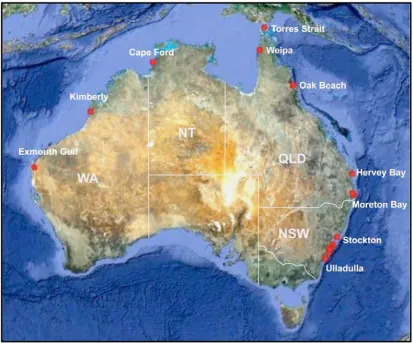
sources from which they were obtained. Table shows the number of fin sets (n) collected from each source (Sample Source). Each fin set was collected from a single shark specimen...23 Table 2.2 All specimens collected for the ‘known’ fin category. For each species the total number

of specimens (n) and, for those specimens with accompanying length data, the size range (total length in cm) is shown. The total number of specimens (n) is further expressed as the number of females (F), males (M) and sex unknown (?). Data from all specimens were collected as images, or as measurements of total length and fin base length (BL). The status of each species (RL), as assessed for The IUCN Red List of Threatened Species™, is shown as Critically Endangered (CR), Endangered (EN), Vulnerable (VU), Lower Risk (LR), Near Threatened (NT), Least Concern (LC), Data Deficient (DD), Not Evaluated (NE)...24 Table 2.3 Fin samples collected for the 'unknown' fin category by vessel. Samples were collected

from illegal foreign fishing vessels apprehended in northern Australian waters between

February 2006 and July 2009...26 Table 2.4. Descriptive characters recorded for all ‘known’ and ‘unknown’ samples of dorsal and

pectoral fins...35 Table 2.5 Description of the five categories used to describe the extent of drying for each shark fin

in the IUU catch. An example image of a dorsal fin sample from each category is provided. Fins are not from the same species. ...38 Table 2.6 Average difference (cm ± SE) of each measurement (A-K), taken from a singe pectoral,

(17)

Table 2.7 Number of dorsal fin samples from foreign fishing vessels by degree of desiccation and vessel type...45 Table 3.1 Summary of all shark specimens for which the denticles of the left side of the dorsal fin

and the dorsal side of the right pectoral fin, at areas C, D, E and H (see Figure 3.3), were examined. For all species investigated, total length range (cm) and total number (n) is given. 59 Table 3.2 The characters used to describe each crown morphology feature on the denticles at areas

C, D, E and F, on both dorsal and pectoral fins. ...61 Table 3.3 Summary of denticle characteristics for each species for skin patch area C (fin tip) on the

dorsal fin. Abbreviations and terms are described in Figure 3.1 and Figure 3.2 and Table 3.2.65 Table 3.4 Summary of denticle characteristics for each species for skin patch area D (anterior

margin) on the dorsal fin. Abbreviations and terms are described in Figure 3.1 and Figure 3.2 and Table 3.1...66 Table 3.5 Summary of denticle characteristics for each species for skin patch area E (posterior

margin) on the dorsal fin. Abbreviations and terms are described in Figure 3.1 and Figure 3.2 and Table 3.2...67 Table 3.6 Summary of denticle characteristics for each species for skin patch area H (free rear tip)

on the dorsal fin. Abbreviations and terms are described in Figure 3.1 and Figure 3.2 and Table 3.2...68 Table 3.7 A summary of the characteristics of the crown morphology of denticles from skin patch

area C (fin tip) taken from the dorsal side of the right pectoral fin for each species.

Abbreviations and terms are described in Figure 3.1 and Figure 3.2 and Table 3.2. ...71 Table 3.8 A summary of the characteristics of the crown morphology of denticles from skin patch

area D (anterior margin) taken from the dorsal side of the right pectoral fin for each species. Abbreviations and terms are described in Figure 3.1 and Figure 3.2 and Table 3.2. ...72 Table 3.9 A summary of the characteristics of the crown morphology of denticles from skin patch

area E (posterior margin) taken from the dorsal side of the right pectoral fin for each species. Abbreviations and terms are described in Figure 3.1 and Figure 3.2 and Table 3.2. ...73 Table 3.10 A summary of the characteristics of the crown morphology of denticles from skin patch

area H (free rear tip) taken from the dorsal side of the right pectoral fin for each species. Abbreviations and terms are described in Figure 3.1 and Figure 3.2 and Table 3.2. ...74 Table 3.11 A summary of the areas on the dorsal fin which can be used to differentiate between the

13 shark species studied, using denticle characters. For each species pair, the area on the fin where denticle morphology differs between those species is given. ...83 Table 3.12 A summary of the areas on the dorsal side of the right pectoral fin which can be used to

(18)

Table 4.1 Summary of the number of dorsal fin samples used to train and test the species

identification protocol. Training refers to specimens used to create the identification protocol. Testing data were used to verify the accuracy of the identification protocol. ‘Known’ refers to samples derived from a whole specimen, which could be identified to species. ‘Unknown’ refers to samples, which were derived from the seized catch of illegal foreign fishing vessels. The species identification of the ‘Unknown’ samples was verified using genetic methods. Some specimens could not be conclusively identified to species using genetic methods, and were grouped into broad categories (grey). As not all specimens had associated total length data, the size range for each species or species group is given as dorsal fin base length (BL) (mm)...99 Table 4.2 A summary of the number of dorsal fin samples which had associated RGB colour data

for both the ‘training’ and ‘testing’ datasets. For each of the samples that did not have colour data (‘No Colour’), the missing RGB colour values were replaced with the average RGB colour values for that species...107 Table 4.3. Key to species and DAGRPs using dorsal fins for northern Australian sharks...111 Table 4.4 The four shark species, Carcharhinus albimarginatus, C. amblyrhynchos, Hemigaleus

australiensis and Triaenodon obesus, and number of dorsal fin samples (n), included in DAGRP1 analysed using discriminant analysis. After initial analysis, all samples of

Carcharhinus albimarginatus and C. amblyrhynchos were pooled to create morphologically similar group 1 (MSG1). DA groups column indicates the groups used in the DA procedure. ...112 Table 4.5 Classification function coefficients derived from Fisher's linear discriminant functions for

DAGRP1. ...113 Table 4.6. Results of direct discriminant analysis of DAGRP1 based on morphometric

measurements for both the original model (including all cases) and the cross-validated model (leave-one-out classification). Bold indicates percent correctly classified...113 Table 4.7 Classification function coefficients derived from Fisher's linear discriminant functions for MSG1...115 Table 4.8 Results of direct discriminant analysis of MSG1 based on HIS colour data for both the

original model (including all cases) and the cross-validated model (leave-one-out

classification). Bold indicates percent correctly classified. ...115 Table 4.9 The four shark species, Eusphyra blochii, Sphyrna mokarran, Rhynchobatus spp., and

Rhynchobatus spp. D2, and number of dorsal fin samples (n), included in DAGRP2 analysed using discriminant analysis. After initial analysis, all samples of Eusphyra blochii and Sphyrna mokarran were pooled to create morphologically similar group 2 (MSG2), and all dorsal and second dorsal fins of Rhynchobatus spp. were pooled to make group RB. DA groups column indicates the groups used in the DA procedure...116 Table 4.10 Classification function coefficients derived from Fisher's linear discriminant functions

(19)

Table 4.11 Results of direct discriminant analysis of DAGR2 based on morphometric measurements for both the original model (including all cases) and the cross-validated model (leave-one-out classification). Bold indicates percent correctly classified. ...117 Table 4.12 Classification function coefficients derived from Fisher's linear discriminant functions

for MSG2. ...118 Table 4.13 Results of direct discriminant analysis of MSG2 based on morphometric measurements

for both the original model (including all cases) and the cross-validated model (leave-one-out classification). Bold indicates percent correctly classified. ...118 Table 4.14 The four shark species, Carcharhinus amblyrhynchoides, C. brevipinna, C. limb/tils and

C. sorrah, and number of dorsal fin samples (n), included in DAGRP3 analysed using

discriminant analysis. DA groups column indicates the groups used in the DA procedure....119 Table 4.15 Classification function coefficients derived from Fisher's linear discriminant functions

for DAGRP3. ...120 Table 4.16 Results of direct discriminant analysis of DAGRP3 based on morphometric

measurements for both the original model (including all cases) and the cross-validated model (leave-one-out classification). Bold indicates percent correctly classified...120 Table 4.17 Classification function coefficients derived from Fisher's linear discriminant functions

for DAGRP4. ...123 Table 4.18 Results of direct discriminant analysis of DAGRP4 based on morphometric

measurements for both the original model (including all cases) and the cross-validated model (leave-one-out classification). Bold indicates percent correctly classified...124 Table 4.19 Classification function coefficients derived from Fisher's linear discriminant functions

for both the original model (including all cases) and the cross-validated model (leave-one-out classification). Bold indicates percent correctly classified. ...126 Table 4.21 The three shark species Carcharhinus cautus, C. leucas and Negaprion acutidens, and

number of dorsal fin samples (n), included in morphologically similar group 4 (MSG4)

analysed using discriminant analysis. ...127 Table 4.22 Classification function coefficients derived from Fisher's linear discriminant functions

(20)

Table 4.24 The two shark species Isurus oxyrinchus and Prionace glauca, and number of dorsal fin samples (n), included in morphologically similar group 5 (MSG5) analysed using discriminant analysis...129 Table 4.25 Classification function coefficients derived from Fisher's linear discriminant functions

for MSG5. ...130 Table 4.26 Results of direct DA of MSG5 based on morphometric measurements for both the

classification). Bold indicates percent correctly classified. ...130 Table 4.27 The three shark species, Galeocerdo cuvier, Rhizoprionodon acutus and Rhizoprionodon

taylori,and number of dorsal fin samples (n), included in morphologically similar group 6 (MSG6) analysed using discriminant analysis....131 Table 4.28 Classification function coefficients derived from Fisher's linear discriminant functions

for MSG6. ...132 Table 4.29 Results of direct DA of MSG6 based on morphometric measurements for both the

classification). Bold indicates percent correctly classified. ...132 Table 4.30 The seven shark species Carcharhinus amblyrhynchoides, C. amblyrhynchos,

C. amboinensis, C. brevipinna, C. dussumieri, C. limb/tils and C. sorrah, and number of dorsal fin samples (n), included in morphologically similar group 7 (MSG7) analysed using

discriminant analysis....133 Table 4.31 Classification function coefficients derived from Fisher's linear discriminant functions

for both the original model (including all cases) and the cross-validated model (leave-one-out classification). Bold indicates percent correctly classified. ...135 Table 4.33 The two shark species Carcharhinus altimus and C. falciformis, number of dorsal fin

samples (n), included in morphologically similar group 8 (MSG8) analysed using discriminant analysis....136 Table 4.34 Classification function coefficients derived from Fisher's linear discriminant functions

for both the original model (including all cases) and the cross-validated model (leave-one-out classification). Bold indicates percent correctly classified. ...137 Table 4.36 The two shark species Carcharhinus altimus and C. falciformis, and number of dorsal

fin samples (n), included in morphologically similar group 9 (MSG9) analysed using

(21)

Table 4.37 Classification function coefficients derived from Fisher's linear discriminant functions for MSG9. ...138 Table 4.38 Results of direct DA of MSG9 based on morphometric measurements for both the

classification). Bold indicates percent correctly classified. ...138 Table 4.39 Contingency table of the classification results (%) of testing samples that were classified

using both the morphological procedure (columns) and the genetic procedure (rows). Bold indicates the percent of samples correctly classified. Grey indicates species that could not be isolated using the genetic procedure and so were grouped together as a species complex (see section 4.2.1. ‘Rationale for the Allocation of Training and Testing Samples’). ...141 Table 4.40 Contingency table of the classification results (%) of testing samples that were classified using both the morphological procedure (columns) and the genetic procedure (rows). The data in this table consists of specimens for which the morphological classification resulted in a posterior probability of > 0.9. Bold indicates the percent of samples correctly classified. Grey indicates species that could not be isolated using the genetic procedure and so were grouped together as a species complex (see section 4.2.1. ‘Rationale for the Allocation of Training and Testing Samples’). ...142 Table 4.41 Total length-dorsal fin base length relationships (sexes combined) for each species (for

which there was sufficient data). TL, total length (cm); BL, dorsal fin base length (mm); n, number of samples; r2, coefficient of determination based on linear regression of (TL) against (BL); SE, standard error of the estimate. ‘Known’ corresponds to whole samples of known species and total length. ‘Photo’ corresponds to samples derived from photographs of whole animals. ...143 Table 5.1 The fifteen illegal foreign fishing vessels from which shark fin catch was sampled and

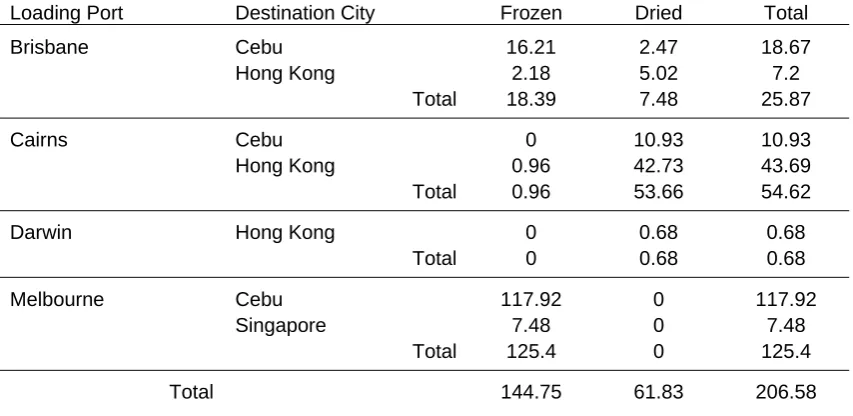
associated data, collected by the Australian Fisheries Management Authority at the time of apprehension. Because of confidentiality issues, vessel names, apprehension dates and specific locations are not provided. Region: Refer to Figure 5.2. Season: SU = Summer, AU = Autumn, WI = Winter, SP = Spring. Type II vessels are traditional Indonesian Perahu sailing vessels, with no alternate form of mechanical propulsion. Type III vessels are all small (< 20 m) motorised vessels, with wooden hulls, from the Indonesian coastal fleet. Steel-hull longliners are large (> 20 m) non-wooden hulled vessels using longline fishing gear. Distance (nm) corresponds to the distance (in nautical miles) between the home port of the vessel and the site where the vessel was apprehended...155 Table 5.2 The estimated catch weight per day for the four Indonesian illegal foreign fishing vessels

for which trip length was known...158 Table 5.3 For each species identified, the parameters (and corresponding literature reference) used

to estimate weight and maturity status of each shark from its total length. The total length of each shark was first estimated from the base length of the dorsal fin (see Chapter 4). ...159 Table 5.4 The contribution by number and estimated biomass and minimum and maximum lengths

(22)

Table 5.5 The percent contribution by number (% n) and estimated biomass (% bm) of each species to the pooled catch per year for both Indonesian and Taiwanese vessels...165 Table 6.1 Summary of all shark specimens used in this study, for each species, and the three

functional groups to which they were assigned. ...180 Table 6.2 The 20 morphological variables used to investigate the morphological properties of the

dorsal, pectoral and caudal fins of all 167 specimens of sharks from 19 species from the family Carcharhinidae. The table shows the abbreviated name, description, and measurements (Figure 6.2) used to derive each morphological variable. ...181 Table 6.3 The average values for each morphological variable for the three ecological groups

oceanic epipelagic, neritic epipelagic, and benthopelagic, represented by 19 species of sharks, belonging to the family Carcharhinidae...185 Table 6.4 Morphological variables identified by SIMPER as typifying the fin morphology of the

carcharhinid species from the oceanic epipelagic, neritic epipelagic, and benthopelagic

functional groups (shaded boxes) and as distinguishing between the fin morphology between the pairwise comparisons of each of the groups (open boxes). ...185 Table 6.5 The classification results for hold-out samples of each of the four stepwise discriminant

analyses using 1) all morphological variables (all fins), 2) morphological variables from the dorsal fin only (dorsal), 3) morphological variables from the pectoral fin only (pectoral), and 3) morphological variables from the caudal fin only (caudal). Results show the percent of samples classified in each category, with correct classifications shown in bold. The number of samples used (n) is shown. Analyses were conducted with the aim of discriminating between the three functional groups, benthopelagic (BP), neritic epipelagic (NE), and oceanic

epipelagic (OE)...189 Table 6.6. Classification function coefficients derived from Fisher's linear discriminant functions

for each of the three functional groups benthopelagic, neritic epipelagic, and oceanic

epipelagic. Classification functions are given for each of the four discriminant analyses...191 Table 9.1 Species identifications for 17 shark dorsal fin tissue samples using three different

identification methods. ‘COI’ corresponds to molecular identifications using the COI region. ‘LM Morphological ID’ corresponds to samples that were identified using morphological techniques. . ‘Control Region’ corresponds to molecular identifications using the control region. *Not included in the Giles study...225 Table 9.2 Tally of specimens (n) assigned to species categories using control region sequences after Ovenden et al., 2007. ...226 Table 9.3 Species identification results for 198 samples from ‘unknown’ dorsal fins collected from

(23)

List of Figures

Figure 1.1 The shark catch of an Indonesian fishing vessel, apprehended in northern Australian waters. Shark catch on such vessels typically consists of excised fins, with the remainder of the carcass discarded at sea. Photo provided by the Australian Fisheries Management Authority (AFMA). ...10 Figure 1.2 Lateral view of a shark showing fins and other external terminology (Last & Stevens

2009). ...11 Figure 2.1 An example of a ‘known’ fin set from a 1.65 m TL, male bull shark (Carcharhinus

leucas). The fins were donated by Australian Seabird Rescue Inc. after the specimen was found dead from a hook injury at Lennox Head, QLD. Known fin sets can contain one, or a combination of the above fins, a) caudal fin, b) second dorsal fin, c) first dorsal fin, d) left pectoral fin (ventral side), e) right pectoral fin (dorsal side), f) anal fin, g) pelvic fin with clasper attached (ventral view) and h) left pelvic fin with clasper attached (dorsal view)...22 Figure 2.2 Map showing the various locations within Australia where specimens from the ‘known’

category of fin samples were obtained. Map sourced from Google Earth...23 Figure 2.3 An example of an illegal Indonesian fishing vessel, which was apprehended in

Australian waters. The vessel contained a cargo of shark fins confiscated by the Australian Fisheries Management Authority (AFMA), and used in this study as part of the ‘unknown’ shark fin category...25 Figure 2.4 Three images of the same dorsal fin sample showing arrangement for photography (a),

and incorrect placing of the free rear tip (b and c)...27 Figure 2.5 The 20 linear distances measured on each dorsal fin for both ‘known’ and ‘unknown’

fins. a) A1 (inner margin), B1 (fin base), C2 (upper anterior margin), D2 (lower anterior margin), E1_{(anterior margin), F}1_{(total fin width), G}2_{(lower posterior margin), H}2_(upper

posterior margin), I1 (posterior margin), M3 (lower outer anterior margin), N3 (upper outer anterior margin). b) J1 (fin height), K1 (direct mid fin height), L1 (absolute fin height), O3 (lower outer posterior margin), P3 (upper outer posterior margin), Q3 (lower inner posterior margin), R3 (upper inner posterior margin), S3 (lower outer free rear tip margin), T3 (upper outer free rear tip margin). 1primary measurements, 2secondary measurements, 3tertiary

(24)

Figure 2.6 The 22 linear distances measured on each pectoral fin for both ‘known’ and ‘unknown’ fins. a) A1 (inner margin), B1 (fin base), C2 ( upper anterior margin), D2 (lower anterior margin), E1 (anterior margin), F1 (total fin width), G2 (lower posterior margin), H2 (upper posterior margin), I1 (posterior margin), M3 (lower outer anterior margin), N3 (upper outer anterior margin). b) J1 (fin height), K1 (direct mid fin height), L1 (absolute fin height), O3 (lower outer posterior margin), P3 (upper outer posterior margin), Q3 (lower inner posterior margin), R3 (upper inner posterior margin), S3 (lower outer free rear tip margin), T3 (upper outer free rear tip margin), U2 (lower inner margin), V2 (upper inner margin). 1primary

measurements, 2secondary measurements, 3tertiary measurements...29 Figure 2.7 Location and terminology of the four primary landmarks on any shark fin from which all

primary measurements are based, for a) dorsal fins (Figure 2.5) and b) pectoral fins (Figure 2.6). Fin ‘‘origin’’ refers to the anterior-most point at which the margin of a fin meets the profile of the body; ‘‘insertion’’ is the posterior-most point of attachment of the base of the fin to the body; “tip” the distal tip or apex, which can be acutely pointed to broadly rounded (see Figure 2.10); “free rear tip” refers to the posterior tip of the fin that is closest to the most posterior point of the fin base. ...30 Figure 2.8 Location of the apex landmarks (white circles) for which all secondary and tertiary

distance measurements are based for a) dorsal and b) pectoral fins. Solid lines represent the original primary (red) or secondary (yellow) measurements and dotted lines represent the largest perpendicular distance from these to the edge of the fin, by which the apex landmark is located. Labels correspond to: A1 (major convex anterior apex), A2 (minor convex anterior apex), A3 (minor convex posterior apex), A4 (minor concave posterior apex), A5 (major concave posterior apex), A6 (concave free rear tip apex), A7 (convex inner margin apex). ....31 Figure 2.9 Height measurements that were calculated from the length measurements in Figure 2.5

Figure 2.6 using Heron’s Formula for a) dorsal fins and b) pectoral fins. Ah (anterior margin height), Bh (posterior margin height), Ch (outer anterior margin height), Dh (outer posterior margin height), Eh (inner posterior margin height), Fh (free rear tip margin height), Gh (inner free rear tip margin height), Hh (free rear tip depth). ...32 Figure 2.10 Examples of fin-tip location on the dorsal fins of shark species with differing tip

shapes. Yellow dot delineates the location of the tip when taking measurements. For pointed fins (a, d and e) the tip is located at the point. For rounded fins (b and c) tip is located at the apex of the rounded edge. ...33 Figure 2.11 Examples of inter-specific variation in fin-tip colour that can occur on both dorsal and

pectoral fins as a) fin-tip colour (1. black, 2. white and 3. no tip colour) and b) nature of fin-tip colour (1. dusky and 2. sharp)...34 Figure 2.12 Relationship between wet and dry values (mm) for each pectoral fin measurement A–U

(n = 26 specimens). Regression lines are included when significant (P ≤ 0.05). Dotted lines show 95% confidence intervals for the regression equation...41 Figure 2.13 The mean change in length after drying for each of the 21 measurements (Figure 2.6)

(25)

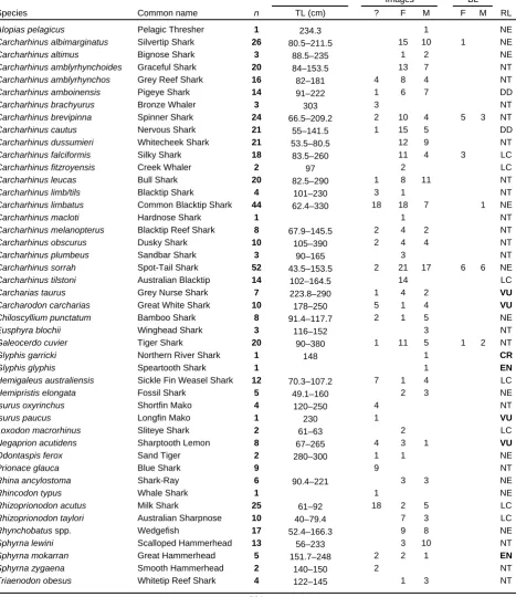
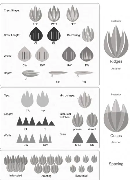
Figure 3.1 Schematic diagrams representing a) denticle crown ridges, cusps, inter ridge spaces, ridge crests and the position of primary and secondary ridge pairs; b) the four crown posterior margin types used to describe the crown posterior margins; c) percent ridge cover is described as the ridge length (rl) as a percentage of the crown length (cl), and; d) the three crown shapes used to describe the overall shape of the denticle crowns. ...54 Figure 3.2 Schematic diagrams representing the summary of denticle characteristics and

abbreviations used to describe the crown morphology of the denticles from each specimen. Abbreviations are explained as follows, a) Ridges. Crest Shape: fine, sharp-edged (FSE), wide,

rounded tops (WRT), broad, flattened plateaus (BFP); Crest Length: cascading length (CL), even length (EL); Width: cascading width (CW), even width (EW), uniform width (UW) tapering width (TW); Depth: uniform depth (UD), tapering depth (TD); Bi-cresting Present: (BC). b) Cusps. Tips: rounded (TR), pointed (TP); Sides: recurved (SRC), straight (SS);

Micro-cusps Present: (MC); Length: even length (EL), cascading length (CL); Width: even width (EW), cascading width (CW); Inter-keel Notches Present: (IKN). c) Spacing.

Imbricated, abutting or separated...55 Figure 3.3 Photographs representing areas from where skin patches were taken for denticle

examination from the a) left side of the dorsal fin and b) dorsal side of the pectoral fin. Each photograph shows anterior and posterior orientation of each fin. C = area C (fin tip), D = area D (anterior margin), E = area E (posterior margin) and H = area H (free rear tip). ...60 Figure 3.4 Photographs taken under light microscope (4-20x magnification) highlighting the

different denticle morphologies of all species at area C on the dorsal fin. Scale bars represent 200 μm. Arrows indicate the direction of anterior to posterior. a) Carcharhinus

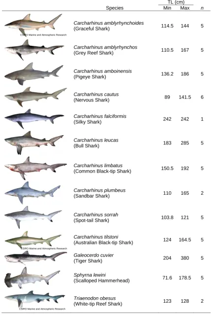
amblyrhynchoides, female, 114 cm TL; b) Carcharhinus amblyrhynchos,female, 167 cm TL c) Carcharhinus amboinensis,female, 152 cm TL ; d) Carcharhinus cautus,female,

114 cm TL; e) Carcharhinus falciformis,male, 242 cm TL; f) Carcharhinus leucas,male, 197.8 cm TL; g) Carcharhinus limbatus,male, 192 cm TL; h) Carcharhinus plumbeus, female, 110 cm TL; i) Carcharhinus sorrah,male, 103.8 cm TL; j) Carcharhinus tilstoni, female, 124 cm TL; k) Galeocerdo cuvier,female, 240 cm TL; l) Sphyrna lewini,female, 173.5 cm TL; m) Triaenodon obesus,male, 123 cm TL. ...75 Figure 3.5 Photographs taken under light microscope (4-20x magnification) highlighting the

different denticle morphologies of all species at area D on the dorsal fin. Scale bars represent 200 μm. Arrows indicate the direction of anterior to posterior. a) Carcharhinus

amblyrhynchoides, female, 114 cm TL; b) Carcharhinus amblyrhynchos,female, 167 cm TL; c) Carcharhinus amboinensis,female, 152 cm TL; d) Carcharhinus cautus,female,

different denticle morphologies of all species at area E on the dorsal fin. Scale bars represent 200 μm. Arrows indicate the direction of anterior to posterior. a) Carcharhinus

(26)

197.8 cm TL; g) Carcharhinus limbatus,male, 192 cm TL; h) Carcharhinus plumbeus, female, 110 cm TL; i) Carcharhinus sorrah,male, 103.8 cm TL; j) Carcharhinus tilstoni, female, 124 cm TL; k) Galeocerdo cuvier,female, 240 cm TL; l) Sphyrna lewini,female, 173.5 cm TL; m) Triaenodon obesus,male, 123 cm TL. ...77 Figure 3.7 Photographs taken under light microscope (4-20x magnification) highlighting the

different denticle morphologies of all species at area H on the dorsal fin. Scale bars represent 200 μm. Arrows indicate the direction of anterior to posterior. a) Carcharhinus

amblyrhynchoides, female, 114 cm TL; b) Carcharhinus amblyrhynchos,female, 167 cm TL; c) Carcharhinus amboinensis,female, 152 cm TL; d) Carcharhinus cautus,female,

different denticle morphologies of all species at area C on the dorsal side of the right pectoral fin. Scale bars represent 200 μm. a) Carcharhinus amblyrhynchoides, female, 114 cm TL; b) Carcharhinus amblyrhynchos,female, 167 cm TL; c) Carcharhinus amboinensis,female, 152 cm TL; d) Carcharhinus cautus,female, 114 cm TL; e) Carcharhinus falciformis,male, 242 cm TL; f) Carcharhinus leucas,male, 197.8 cm TL; g) Carcharhinus limbatus,male, 192 cm TL; h) Carcharhinus plumbeus,female, 110 cm TL; i) Carcharhinus sorrah,male, 103.8 cm TL; j) Carcharhinus tilstoni,female, 124 cm TL; k) Galeocerdo cuvier,female, 240 cm TL; l) Sphyrna lewini,female, 173.5 cm TL; m) Triaenodon obesus,male, 123 cm TL. ...79 Figure 3.9 Photographs taken under light microscope (4-20x magnification) highlighting the

different denticle morphologies of all species at area D on the dorsal side of the right pectoral fin. Scale bars represent 200 μm. Arrows indicate the direction of anterior to posterior. a) Carcharhinus amblyrhynchoides, female, 114 cm TL; b) Carcharhinus amblyrhynchos, female, 167 cm TL; c) Carcharhinus amboinensis,female, 152 cm TL; d) Carcharhinus cautus,female, 114 cm TL; e) Carcharhinus falciformis,male, 242 cm TL; f) Carcharhinus leucas,male, 197.8 cm TL; g) Carcharhinus limbatus,male, 192 cm TL; h) Carcharhinus plumbeus,female, 110 cm TL ; i) Carcharhinus sorrah,male, 103.8 cm TL; j) Carcharhinus tilstoni,female, 124 cm TL; k) Galeocerdo cuvier,female, 240 cm TL; l) Sphyrna lewini, female, 173.5 cm TL; m) Triaenodon obesus,male, 123 cm TL. ...80 Figure 3.10 Photographs taken under light microscope (4-20x magnification) highlighting the

(27)

Figure 3.11 Photographs taken under light microscope (4-20x magnification) highlighting the different denticle morphologies of all species at area H on the dorsal side of the right pectoral fin. Scale bars represent 200 μm. Arrows indicate the direction of anterior to posterior. a) Carcharhinus amblyrhynchoides, female, 114 cm TL; b) Carcharhinus amblyrhynchos, female, 167 cm TL; c) Carcharhinus amboinensis,female, 152 cm TL; d) Carcharhinus cautus,female, 114 cm TL; e) Carcharhinus falciformis,male, 242 cm TL; f) Carcharhinus leucas,male, 197.8 cm TL; g) Carcharhinus limbatus,male, 192 cm TL; h) Carcharhinus plumbeus,female, 110 cm TL; i) Carcharhinus sorrah,male, 103.8 cm TL; j) Carcharhinus tilstoni,female, 124 cm TL; k) Galeocerdo cuvier,female, 240 cm TL; l) Sphyrna lewini, female, 173.5 cm TL; m) Triaenodon obesus,male, 123 cm TL. ...82 Figure 4.1 Example photograph of a shark fin sample containing a scale, specimen number and the

standard blue mat used to standardise RGB colour values. ...101 Figure 4.2 Flow diagram outlining the approach taken to identify dorsal fins, from 93 fin samples

from the testing group, from 13 species of shark found in northern Australian waters. A dichotomous key is used to identify the dorsal fin sample to either species or discriminant analysis group (DAGRP). Classification equations (generated for each DAGRP) are then used to identify the fin to either species or morphologically similar group (MSG). MSGs are then identified to species or another MSG, until the dorsal fin was identified to species. Arrows with closed lines represent where fin colour, fin-tip colour or simple primary measurements are used for classification, arrows with broken lines represent where DA equations are used for classification...102 Figure 4.3 a) The five height measurements calculated from lengths in Figure 4.4 using Heron’s

Formula (Equations 1 and 2). Ah (anterior margin height), Bh (posterior margin height), Ch (outer anterior margin height) Dh (outer posterior margin height), Eh (inner posterior margin height), Fh (free rear tip margin height), Gh (inner free rear tip margin height), Hh (free rear tip depth); b) Location of the primary (orange circles) and apex (white circles) landmarks for which all primary, secondary and tertiary distance measurements are based. Solid lines represent the original primary (red) or secondary (yellow) measurements and dotted lines represent the largest perpendicular distance from these to the edge of the fin, by which the apex landmark is located. Labels correspond to: 1. fin origin, 2. fin-tip, 3. free rear tip, 4. fin insertion A1 (major convex anterior apex), A2 (minor convex anterior apex), A3 (minor convex posterior apex), A4 (minor concave posterior apex), A5 (major concave posterior apex), A6 (concave free rear tip apex)...104 Figure 4.4 The 17 linear distances measured on each dorsal fin. a) A1_{(inner margin), B}1_{(fin base),}

C2 (upper anterior margin), D2 (lower anterior margin), E1 (anterior margin), F1 (total fin width), G2 (lower posterior margin), H2 (upper posterior margin), I1 (posterior margin), M3 (lower outer anterior margin), N3 (upper outer anterior margin). b)J1 (fin height), K1 (direct mid fin height), L1 (absolute fin height), O3 (lower outer posterior margin), P3 (upper outer posterior margin), Q3 (lower inner posterior margin), R3 (upper inner posterior margin), S3 (lower outer free rear tip margin), T3 (upper outer free rear tip margin). 1primary

measurements, 2secondary measurements, 3tertiary measurements...105 Figure 4.5 Shows how each of the 35 species were divided into the 4 DAGRPs and nine MSGs

(28)

Figure 4.6 Discriminant function scores for the 53 dorsal fin samples in DAGRP1 showing the how the first two functions discriminate between the three groups using the linear measurements L, J and R. Symbols: , MSG1; , Hemigaleus australiensis; , Triaenodon obesus...114 Figure 4.7 Three-dimensional plot of the first 3 discriminant functions from a canonical DA of

morphological measurements from the dorsal fins of 142 dorsal fin samples from four known species of which DAGRP3 comprises. Symbols: , Carcharhinus amblyrhynchoides; ,

C. brevipinna; , C. limbatus/tilstoni; , C. sorrah. ...121 Figure 4.8 The 21 species groups included in DAGRP4 and their allocation to the four

morphologically similar groups MSG3, MSG4, MSG5, and MSG6. MSG3 was further divided into three morphologically similar groups, MSG7, MSG8, and MSG9. ...122 Figure 4.9 Three-dimensional plot of the first 3 discriminant functions from a canonical

discriminant analysis of morphological measurements and colour data from the dorsal fins of 408 dorsal fin samples from four morphologically similar groups ( MSG3, MSG4, MSG5, MSG6) of which DAGRP4 comprises...124 Figure 4.10 Two-dimensional plot of the first two discriminant functions derived from a canonical

discriminant analysis, using morphological measurements and colour data, of 295 dorsal fin samples from the three morphologically similar groups (MSG7, MSG8, MSG9), derived from MSG3...126 Figure 4.11 Two-dimensional plot of the first two discriminant functions derived from a canonical

discriminant analysis, using morphological measurements and colour data, of 55 dorsal fin samples from the three species derived from MSG4 (Carcharhinus cautus, C. leucas and

Negaprion acutidens)...129 Figure 4.12 Three two-dimensional plots of the first six discriminant functions derived from a

canonical discriminant analysis, using morphological measurements and colour data, of 190 dorsal fin samples from the seven species derived from MSG7...135 Figure 4.13 Three-dimensional plot of the first three discriminant functions derived from a

canonical discriminant analysis, using morphological measurements and colour data, of 75 dorsal fin samples from the four species (Carcharhinus obscurus, C. plumbeus, Sphyrna lewini, S. zygaena) of which MSG9 comprises. ...139 Figure 4.14 An ‘unknown’ fin set, from the seized catch of an Indonesian fishing vessel that was

apprehended fishing illegally in northern Australian waters. The image shows how fins from the same shark (in this case the dorsal, lower caudal and left and right pectoral fins from a tiger shark (Galeocerdo cuvier)) are often tied together for drying...145 Figure 4.15 The left pectoral fins from two species of hammerhead shark, a) Sphyrna lewini dorsal

view and b) ventral view; c) Sphyrna zygaena dorsal view and d) ventral view...147 Figure 5.1 The number of illegal foreign fishing vessels (mostly Indonesian) apprehended in the

(29)

Figure 5.2 Location where each vessel was apprehended for the 12 foreign fishing vessels that had associated data (). The four regions used for multivariate analysis are pictured: W (western region), N (northern region), TS (Torres Strait region), and E (eastern region) (Table 5.1). Two of the twelve vessels were apprehended in the same location, thus only 11 are visible (depicted by *). ...156 Figure 5.3 Pooled estimated length frequency histograms and maturity data for all shark species

from a) the 15 Indonesian illegal foreign fishing vessels, and b) the two Taiwanese illegal foreign fishing vessels. Shades represent estimated maturity status, immature (), maturing () and mature (). Length represents total length (cm)...163 Figure 5.4 Length frequency histograms for the 31 species for which total length (TL) could be

estimated from the catch of 15, both Indonesian and Taiwanese, foreign fishing vessels apprehended in northern Australia between February 2006 and July 2009. Colours represent estimated maturity status, immature (), maturing () and mature (). Length represents total length (cm) for all species except Alopias superciliosus where length represents fork length (cm). ...166 Figure 5.5 Shark catch in northern Australian waters in 2006. Dark bars () represent the reported

shark catch for the three main commercial shark fisheries in northern Australia, the Northern Territory Offshore Net and Line Fishery (NTONL) (Buckworth & Beatty 2008), Queensland Gulf of Carpentaria Inshore Fin Fish Fishery (QGoCIFFF) (Roelofs 2009) and the Western Australia Joint Authority Northern Shark Fishery (WAJANSF) (McCauley, et al. 2000). Light bar () represents the estimated Illegal Unregulated and Unreported (IUU) catch by Indonesian foreign fishing vessels...172 Figure 6.1 Schematic diagram demonstrating the hydrodynamic forces of a) roll, b) yaw, and c)

pitch, acting on the shark body during swimming...176 Figure 6.2 The morphometric measurements taken from the a) dorsal, b) left pectoral, and c) caudal

fins of each of the 167 shark specimens from 19 species from the family Carcharhinidae. These measurements were used to construct the 20 morphological variables used in the

multivariate analysis (Table 6.2)...182 Figure 6.3 A non-metric multidimensional scaling (MDS) ordination derived from morphological

data (consisting of 20 morphological variables) from the dorsal, pectoral and caudal fins of each of the 167 specimens from 19 shark species (family: Carcharhinidae). The same MDS ordination is shown twice, indicating a) the factor ‘functional group’, and b) the factor

‘species’. ...186 Figure 6.4. Three-dimensional plot of the results of four stepwise discriminant analyses using a) all

(30)

1

1 Shark-finning: The problem and the

solution

1.1 Introduction

It has been ten years since the United Nations Food and Agriculture organisation (FAO)

implemented an International Plan of Action for the Conservation and Management of Sharks

(IPOA Sharks) because of concern about expanding global shark catch and the potential negative

impacts on shark populations worldwide. Since that time, 466 shark species from 34 families have

been assessed for the International Union for Conservation of Nature(IUCN) Red List of

Threatened Species, ten shark species have been listed under the Convention On International Trade

(31)

(CMS) and, in Australia, 13 have been listed under the Environment Protection and Biodiversity

Conservation Act (EPBC act). Of the 466 shark species that have been assessed by the IUCN Red

List, 15.6% were found to be Critically Endangered, Endangered or Vulnerable, 14.8% were Near

Threatened and 44% were Data Deficient (IUCN 2009).

Despite global concern for the vulnerability of many sharks to overfishing, the level of

reported catch remains high − with actual mortality estimated to be three times higher, attributed to

illegal fishing, under-reporting and unregulated fishing (Camhi, et al. 1998, Clarke, et al. 2006).

Because of the aforementioned concerns, it has been suggested that the truest estimate of fishing

mortality can be obtained by examining trade data (Baker 2008). In the case of many shark species,

this means quantifying shark catch as represented by the most retained product, shark fin.

This chapter will review the rationale for, developments of, and challenges to management

since the implementation of IPOA Sharks, using Australian shark fisheries as an example.

Secondly, this chapter will provide suggestions for obtaining more robust catch data via the

quantification of shark mortality as represented by shark fin catch.

1.2 Concern for Shark Stocks

The importance of large predators, such as sharks, to marine ecosystems has been a topic widely

discussed and documented in the literature (Duffy 2002, Estes, et al. 1998, Olsen 1959, Pace, et al.

1999, Paine 1980). Despite what is already known about tropic cascades there is still uncertainty

about the effect of removing apex predators from marine food webs (Atz 1964, Bascompte, et al.

2005, Frank, et al. 2005, Pace, et al. 1999, Stevens, et al. 2000, Strong 1992). However, it is agreed

that detrimental top down effects must be widely expected whenever entire functional groups of

predators are removed (Estes, et al. 1998, Frid, et al. 2008, Myers, et al. 2007, Schindler, et al.

2002).

(32)

a low resilience to fishing mortality and an increased susceptibility to overfishing, due to K-selected

life-history traits such as late maturation, low fecundity, and slow growth rates (Barker &

Schluessel 2005, Camhi, et al. 1998, Frisk, et al. 2001, Hoenig & Gruber 1990, Holden 1974,

Musick 2000, Smith, et al. 1998, Stevens, et al. 2000). Furthermore, for shark species with

restricted distributions, and those that aggregate by age, sex, and reproductive state, this

susceptibility is exacerbated (Baum, et al. 2003, Bonfil 1994, Graham, et al. 2001, Jukic-Peladic, et

al. 2001, Musick 1999). Differential vulnerability to fishing pressure exists among shark and ray

species, with species exhibiting large body sizes and low productivity generally being the most

vulnerable (Cortes 1998, Stevens, et al. 2000) while some smaller, more fecund species such as the

Gummy Shark (Mustelus antarcticus) can be harvested sustainably (Pribac, et al. 2005, Walker

1998). In western North Atlantic shark fisheries, populations of large slow growing shark species,

such as the Sand Tiger (Odontaspis taurus), and Dusky Shark (Carcharhinus obscurus), have

collapsed and show little sign of recovery. However, in the same fishery, faster growing and more

fecund species such as the Sandbar Shark (Carcharhinus plumbeus), have enabled the fishery to

continue, despite also showing signs of population reduction (Musick 1999, Musick, et al. 1993).

Such examples illustrate the necessity of species-specific shark data collection and assessment for

(33)

Box 1.1 Examples of Collapsed Shark Stocks: Myers & Worm (2003) estimate that the biomass of large predatory fish in the world’s oceans is only about 10% of what it was at

pre-industrial levels. They also predict that declines of large predators in coastal regions are

extending throughout the open ocean which could have potentially serious consequences for

entire marine ecosystems (Myers & Worm 2003). A recent example of this is in the Gulf of

Mexico, where Oceanic Whitetip (Carcharhinus longimanus) and Silky Sharks (Carcharhinus

falciformis) have declined by over 99 and 90%, respectively (Baum & Myers 2004). Furthermore

in the Atlantic, coastal shark populations have declined by up to 85% in the past two decades

(Baum, et al. 2003, Camhi, et al. 1998), and in the USA, large coastal sharks are estimated to

have declined from 8.9 million sharks in 1974 to around 1.4 million in 1998 (NMFS 1999).

Well-documented species-specific examples of collapsed shark fisheries are the Porbeagle (Lamna

nasus) fishery in the North Atlantic (Campana, et al. 2008), the School Shark (Galeorhinus

galeus) fisheries off California and south eastern Australia (Olsen 1959, Punt & Walker 1998,

Ripley 1946), most worldwide Basking Shark (Cetorhinus maximus) fisheries (Parker & Stott

1965) and the Spiny Dogfish (Squalus acanthias) fisheries both in the North Sea and off British

Columbia (Holden 1968, Ketchen 1975).

Despite the necessity for species-specific catch data for shark management, very little

archival, and almost no species-specific data on historical catches and landings for most shark

species exist as historically shark products have been of low interest (Barker & Schluessel 2005,

Castro, et al. 1999, Shotton 1999a, Shotton 1999b). In the last 15 years, more than 12 million

tonnes (810 000 tonnes per annum) of sharks and rays have been reported by target fisheries

throughout the world (Last & Stevens 2009). Despite such estimates of world shark catch, in 1997

chondrichthyan landings accounted for only 0.87% of the total world fish catch, with sharks

comprising approximately half of this total (FAO 2002). As this represents only a small proportion

of world fish catch, and therefore a small percentage of individual countries marine fisheries, sharks

and rays have historically received low priority and limited resources for management purposes

(FAO 2000, Musick 2000). With current rates of exploitation driven by the rising demand for

highly priced shark fins, this proportion is beginning to increase. However, because shark fin

represents the only lucrative economic windfall in shark fisheries, these fisheries continue to be a

low priority for conservation and research (Barker & Schluessel 2005). Clarke et al. (2006) estimate