220
Reihe Ökonomie
Economics Series
Too Old to Work, Too Young
to Retire?
Andrea Ichino, Guido Schwerdt, Rudolf Winter-Ebmer,220
Reihe Ökonomie
Economics Series
Too Old to Work, Too Young
to Retire?
Andrea Ichino, Guido Schwerdt, Rudolf Winter-Ebmer,Josef Zweimüller October 2007
Contact: Andrea Ichino
Dipartimento di Scienze Economiche Universita' di Bologna
Piazza Scaravilli 2, 40126 Bologna, Italy email: [email protected] Guido Schwerdt
Ifo Institute for Economic Research Department Human Capital and Innovation Poschingerstraße 5 81679 Munich, Germany email: [email protected] Rudolf Winter-Ebmer Department of Economics University of Linz 4040 Linz, Austria email: [email protected] and
Department of Economics and Finance Institute for Advanced Studies Stumpergasse 56
1060 Vienna, Austria Josef Zweimüller
Institute for Empirical Research in Economics University of Zurich
Bluemlisalpstrasse 10 8006 Zuerich, Switzerland email: [email protected]
Founded in 1963 by two prominent Austrians living in exile – the sociologist Paul F. Lazarsfeld and the economist Oskar Morgenstern – with the financial support from the Ford Foundation, the Austrian Federal Ministry of Education and the City of Vienna, the Institute for Advanced Studies (IHS) is the first institution for postgraduate education and research in economics and the social sciences in Austria. The Economics Series presents research done at the Department of Economics and Finance and aims to share “work in progress” in a timely way before formal publication. As usual, authors bear full responsibility for the content of their contributions.
Das Institut für Höhere Studien (IHS) wurde im Jahr 1963 von zwei prominenten Exilösterreichern – dem Soziologen Paul F. Lazarsfeld und dem Ökonomen Oskar Morgenstern – mit Hilfe der Ford-Stiftung, des Österreichischen Bundesministeriums für Unterricht und der Stadt Wien gegründet und ist somit die erste nachuniversitäre Lehr- und Forschungsstätte für die Sozial- und Wirtschafts-wissenschaften in Österreich. Die Reihe Ökonomie bietet Einblick in die Forschungsarbeit der Abteilung für Ökonomie und Finanzwirtschaft und verfolgt das Ziel, abteilungsinterne Diskussionsbeiträge einer breiteren fachinternen Öffentlichkeit zugänglich zu machen. Die inhaltliche Verantwortung für die veröffentlichten Beiträge liegt bei den Autoren und Autorinnen.
Abstract
We use firm closure data for Austria 1978-1998 to investigate the effect of age on employment prospects. We rely on exact matching to compare workers displaced by firm closure with similar non-displaced workers. We then use a difference-in-difference strategy to analyze employment and earnings of older relative to prime-age workers in the displacement and non-displacement groups. Results suggest that immediately after plant closure the old have lower re-employment probabilities as compared to prime-age workers but later they catch up. While among the young the employment prospects of the displaced remain persistently different from those of the non-displaced, among the old the effect of displacement fades away, and actually disappears even immediately after plant closure when the effect of tenure based severance payment is controlled for. Our evidence suggests that increasing the retirement age does not necessarily produce individuals who are "too old to work but too young to retire".
Keywords
Aging, Employability, Plant Closures, Matching
JEL Classification J14, J65
Comment
This research has profited from comments by seminar participants in Amsterdam, Berkeley, LSE, NBER, EALE, Padova, Rimini, St. Gallen, Stockholm, Tübingen, and Vienna. We gratefully acknowl-edge financial support from the Austrian Science Foundation (FWF) and the Austrian National Bank under the project No. 10643. We received insightful comments from David Card and Enrico Moretti to whom our gratitude goes. We would also like to thank Oliver Ruf for excellent research assistance in
Contents
1 Introduction
1
2 Productivity
and
wages over the life cycle
3
3
Data and matching strategy
5
4 Results
7
4.1 Descriptive evidence ... 8 4.2 Controlling for observed heterogeneity ... 12
5 Discussion
and
robustness checks
17
5.1 Data and model specification ... 17 5.2 The role of institutions ... 19 5.3 A suggested behavioral interpretation ... 23
6 Conclusion
24
References 26
1
Introduction
In most industrialized countries the labor force is aging because of both lower fertility rates and longer life expectancy. These developments lead to worries about the solvency of pay-as-you-go pension systems which in turn have induced pension reforms aimed at increasing minimum retirement age. The feasibility of keeping up the employment prospects of an increasingly older workforce is, however, questionable. From a public finance point of view, high unemployment rates of older workers would take away much of the gains of increases in retirement age.
Since wages and working conditions in ongoing jobs are characterized by long term implicit contracts1 and because of regulations in terms of firing
re-strictions and wage adjustments, the employment prospects of older workers are best investigated in a situation where the worker faces the job market af-ter a displacement or plant closure. This kind of events offer the opportunity to compare what happens to old and young workers when they are exoge-nously thrown into the labor market. After displacement, the employment opportunities of a worker will depend on possible productivity changes due to aging (a demand effect), but also on the supply reaction of the worker in terms of search intensity and the willingness to accept wage concessions. If lower productivity of older workers decreases their market wage over time, their search intensity might fall, because searching for a not-so-good-any-more job is not really worthwhile. On the other hand, older workers might have a higher discount rate: they have fewer years in front of them to earn a labor income that would be higher than retirement income, and moreover they face a higher probability of death. This greater impatience of older workers makes them more willing to accept wage concessions in order to find a new job faster. Institutions, like for example severance payments and pen-sion regulations, may also distort supply and demand behaviour. Depending on the relative strength of these counteracting effects, employment rates of older workers after displacement could be higher or lower as compared to prime-age workers, relative to what would have happened in the absence of
displacement.
In this paper we look at relative employment rates of older workers in Austria. Based on social security data for the entire Austrian workforce, we rely on exact matching to compare workers displaced due to a plant closure with a control group of non-displaced workers. The huge size of the data set at our disposal (more than 1 million persons) enables us to exploit exact matching techniques in very favorable conditions that are rarely met in studies based on these methods. Within this matched sample, we extend the standard displacement cost specification introduced by Jacobson et al. (1993) and use a difference-in-difference strategy to look at the employment and earnings prospects of older relative to prime-age workers in the displacement and non-displacement groups.
Our identification assumption is that the counterfactual of the displaced workers at any age, are the (almost exactly matched) non-displaced workers. The causal effect of being displaced at an older age as opposed to a younger age is identified by how the difference of the employment and earnings profiles of displaced and non-displaced workers change with age. Note that this estimation strategy combines the advantages of exact matching to improve the comparability of treated and control subjects, with the advantages of differencing in panel data to control for remaining confounders captured by time invariant individual, cohort and time effects. Results suggest that within ten years after plant closure both displaced prime-age and older workers have significantly lower employment rates as compared to their respective control groups. More surprisingly, with respect to the benchmark represented by workers never displaced in the corresponding age cohort, older workers have lower employment rate than prime-age workers immediately after plant closure, but they manage to catch up over time.
These results can be interpreted as evidence that after plant closure older workers are considered less productive by the market but are reluctant to lower their reservation wages enough to ensure the same employability of the young, possibly because of the higher severance payments to which they are entitled. With the passage of time, the shorter time horizon of the old induces them to lower their reservation wage in order to find a job before
retiring, and this explains the observed catching up.
The remainder of this paper is organized as follows: Section 2 gives an overview of the related literature on productivity and wage effects over the life cycle. Section 3 describes the data and the matching procedure. Sec-tion 4 presents some descriptive evidence, the identificaSec-tion strategy and the econometric estimates. Section 5 discusses the robustness of these results and possible interpretations, while Section 6 concludes.
2
Productivity and Wages over the Life Cycle
Human capital theory predicts a concave life cycle age-productivity profile due to skill obsolescence as aging progresses and to a shorter horizon later in life, which reduces the incentive for learning. Empirical wage studies in the Mincer tradition have typically found such a concave pattern. However, while earnings are much easier measured than productivity as such, they are not necessarily a good proxy for productivity over the life cycle for a variety of reasons. Models of firm-specific training imply that firms participate in paying for training in the early part of the careers, making wages higher than productivity early on. These initial investments will later be repaid by agreeing on lower wages. A testable prediction of these models is that layoff-probabilities of older workers are lower. An alternative hypothesis concentrates on incentive effects: incentives to work hard close to retirement age can only be kept up if wages exceed productivity. In this case, shirking workers would experience a major loss in case of dismissal and this prospect would keep up their effort at work (Lazear (1979)). These studies in general indicate that wages in ongoing jobs are likely not to be a good proxy of current productivity.
There are many direct studies on particular aspects of productivity mainly done by social psychologists who look at specific tasks, like cognitive abilities, finger dexterity, verbal skills, and the productivity of learning at higher age.2
2See Skirbekk (2004) for a survey. Highly specific studies look at productivity at sports
activities or chess (Fair (2004)) or the productivity of researchers in science (Stephan and Levin (1988)) and economics (Oster and Hamermesh (1998)). In both cases a significant negative age-gradient has been found.
The general message is that productivity reductions at older ages are partic-ularly strong when problem solving, learning and speed as well as physical strength are important, while older individuals maintain a relatively high pro-ductivity level in work tasks where verbal abilities and organizational skills matter more. Even if the negative effects of task-specific aging are widely documented, overall productivity in a job depends not only on being quick and adept in specific tasks, but also on experience and on a better knowledge of processes and firms’ organization.
Direct tests on productivity are also based on piece rate schemes and supervisors’ ratings. While those based on piece rates typically find quite substantial decreases in productivity with age, supervisors’ ratings often im-ply the opposite. Both methods are not fully satisfactory: results from piece rates are not easily generalizable because they relate to very specific jobs, mainly manual occupations or simple clerical work like typing. A general disadvantage with the use of supervisors’ ratings to rank individuals by age and productivity is that managers often may wish to reward older workers for their loyalty and past achievements (Skirbekk (2004)).
In recent years the use of matched employer-employee data sets has al-lowed to study the impact of the workforce’s age structure on productivity or sales. Most of these studies3 find concave age-productivity profiles but
in many cases these profiles are flatter than the corresponding age-earnings profiles. While matched employer-employee data offer great opportunities to combine personal with firm information, the main challenge of these ap-proaches is to isolate the effect of workers’ age on productivity from other influences, in particular the selectivity of workers’ types: good workers get promoted, whereas bad workers will loose their jobs, a problem which will get more severe as the workforce ages. Moreover, more successful firms will increase their payroll, with obvious effects on the age structure of the work-force.
These age-productivity issues are relevant for the interpretation of the relationship between age and risk of job displacement. Kuhn (2002) in a
3See for instance Hellerstein and Neumark (2004), Haltiwanger and Spletzer (1999) or
collaborative study on worker displacement finds (see page 49) no direct effect of age on the risk to be displaced from a job. On the other hand, some studies show that the risk of job loss is in fact greater among older workers when the rate of technological change is highest (Bartel and Sicherman (1993), Ahituv and Zeira (2000)).
Our paper produces new evidence on these issues, based on a carefully designed identification strategy described in the next section.
3
Data and matching strategy
We use administrative employment records from the Austrian Social Secu-rity Database (ASSD). The data set includes the universe of private sector workers in Austria covered by the social security system. All the employment records can be linked to the establishment in which the worker is employed. The data set covers the years 1978 to 1998. Daily employment and monthly earnings information is very reliable, because social security tax payments for firms as well as benefits for workers hinge on these data.4 Monthly earnings are top-coded, which applies to approximately 10% of workers. We trans-formed monthly gross earnings in daily wages by dividing them by effective employment duration in each month of observation.
We concentrate on all workers employed in the period 1982 to 1988, who are therefore at risk of a firm5 breakdown in this period; this allows us to
observe the workers in detail for 4 years prior to potential bankruptcy and for 10 years afterwards. We exclude firms from the construction and tourism industries, because in these sectors seasonal unemployment is very high and firms often close down out of season to reopen after several months with the same workforce. Moreover, we restrict ourselves to workers coming from firms with more than 5 employees at least once during the period 1982 and 1988 and having at least one year of tenure at their firm. To study the aging process we compare two cohorts: those of age 35 to 44 at the time of
4See Hofer and Winter-Ebmer (2003) for a description of the data set.
5Although establishments, and not firms, are our units of observation for the
iden-tification of plant closures, we will use interchangeably these words for simplicity and convenience.
displacement – the “young” - and those between 45 and 55 – the “old”. Each establishment has an employer social security number. Hence, an exit of an establishment in the data occurs when the employer identifier ceases to exist. However, some of these cases are not true firm exits, and (most of the) employees continue under a new identifier, for example because of a takeover in a family business or other similar reasons. If more than 50% of the employees continue under a new employer identification number we do not consider this a failure of the establishment.6
Our treatment group for the matching procedure consists of 11,578 work-ers from firm deaths between 1982 and 1988. Our control group comprises workers from all firms not going bust between 1982 and 1988, with the same tenure, industry and age requirements as the treated; this group consists of 1,087,705 workers. Our data set is ideal for matching. We have quarterly in-formation for all workers over the four years before plant closure and have the universe of Austrian workers available as a potential control group. Detailed past work histories, i.e. employment record and earnings, can be considered an almost sufficient statistic for the set of unobservable characteristics of workers (see for example Card and Sullivan (1988)).
Our matching procedure is therefore very simple: We perform exact matching between the treated and control subjects on the following crite-ria: sex, age, broad occupation (blue- or white-collar), location of firm (9 provinces), industry (30 industries), employment history in each of the quar-ters 4, 5, 6 and 7 before plant closure.7 We do almost exact matching on
continuous variables: average daily wages in the quarters 8, 9, 10 and 11 be-fore plant closure are matched by decile group8 and firm size in the two years
before plant closure is matched by quartile groups. Thus, for each treated subject, our matching algorithm has to find a control subject with identical characteristics (according to the list mentioned above) at the date of plant closure. Applying this matching procedure we are able to identify at least
6Workers from such firms are coded as “ambiguous” and are neither in the treatment
nor the control group.
7Note that we only use persons with tenure longer than one year in the current firm. 8We do not want to match earnings too close to firm failure, because there might be
one control subject for 6,630 treated subjects (out of a total of 11,578 sub-jects in the plant closure sample).9 In total we end up with 36,677 matched
controls.
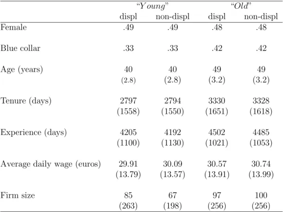
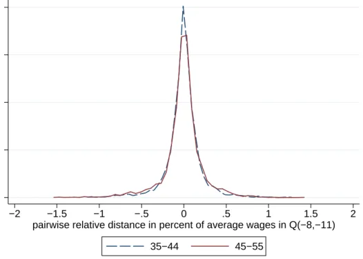
Table 1 gives descriptive statistics about the quality of the matching. Whereas gender, blue-collar and age are exactly matched, tenure and work experience (only available since 1972) were not among the matching variables in our algorithm. It is therefore reassuring to see, that our matching strategy works perfectly in terms of tenure and work experience: mean differences between treated and controls are only marginal. Similarly, for average daily wages, which have been matched by deciles in the quarters 8 to 11 prior to plant closure, the differences are very small. Figure 1 shows that this small difference in means does not hide large individual differences between pairs: kernel density estimates for the relative distance in average wages in the quarters -8 to -11 show that both for old and young workers, most of the density is in the region between plus and minus a quarter of a percent. Considering firm size, the difference is again very small for old workers and only slightly larger for young workers.
4
Results
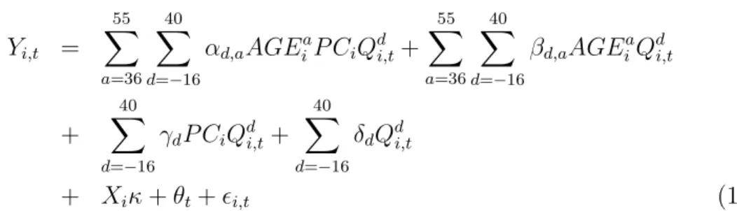
The most general specification of our estimation problem is the following.
Yi,t = 55 X a=36 40 X d=−16
αd,aAGEiaP CiQdi,t+
55 X a=36 40 X d=−16 βd,aAGEiaQ d i,t + 40 X d=−16 γdP CiQdi,t+ 40 X d=−16 δdQdi,t + Xiκ+θt+i,t (1)
where: Yi,tis the outcome of interest(employment status or wage); idenotes
workers; t is calendar time measured in quarters; AGEia is a dummy taking value 1 if worker i has age a, with a ∈ [35,55]10; P Ci is a dummy taking
9We experimented also with less restrictive matching algorithms that increase the
num-ber of matches without major quantitative changes in the results.
10Note that the summation running over a goes from 36 to 55 because the first age
value 1 ifi is displaced in a plant closure; d is the distance in quarters from potential or actual plant closure, which ranges in the data from −16 to 40 with 0 denoting the last quarter before plant closure; Qd
i,tis a dummy taking
value 1 if i is observed in quarter t at a distance of d quarters from plant closure; Xi are pre-plant closure observable characteristics of i (including
age); i,t capture unobservables of i at quarter t and αd,a, βd,a, γd, δd, κ and
the calendar time effectsθtare the parameters that we would like to estimate.
This specification makes clear the nature of our identification assumption. The counterfactual of the displaced workers, at any age, are the non-displaced workers. The causal effect of being displaced at an older age as opposed to a younger age is identified by how the difference of the employment profiles of displaced and non-displaced change with age. To keep the problem man-ageable and results interpretable, we simplify this general specification as described below.
4.1
Descriptive evidence
In order to obtain a preliminary graphical image of the effect of age on the comparison between displaced and matched non-displaced subjects before and after the plant closure date, we collapse the 21 age dummiesAGEa
i into
a binary dummy OLDi defined as
OLDi = 1 if a∈[45,55], 0 if a∈[35,44]. (2)
In this way we concentrate our analysis on the comparison of the employ-ment and earnings prospects of older relative to prime-age workers in the displacement and non-displacement groups. Thus, equation 1 simplifies to
Yi,t = 40 X d=−16 αdOLDiP CiQdi,t+ 40 X d=−16 βdOLDiQdi,t (3) + 40 X d=−16 γdP CiQdi,t+ 40 X d=−16 δdQdi,t+θt+i,t
Panel A and B of Figure 2 report, respectively for the young and the old, the average employment rates of the displaced and non displaced workers as a function of the distance from plant closure d, defined as follows using equation 3:
E(Yi,t|OLDi = 0, P Ci = 0, Qdi,t= 1) = δd
E(Yi,t|OLDi = 0, P Ci = 1, Qdi,t= 1) = δd+γd
E(Yi,t|OLDi = 1, P Ci = 0, Qdi,t= 1) = δd+βd
E(Yi,t|OLDi = 1, P Ci = 1, Qi,td = 1) = δd+βd+γd+αd.
By construction, the employment rates of both the treated and the matched control observations are equal to unity in the four quarters prior to the plant closure date. The employment rates at earlier dates show that our matching procedure works perfectly as measured by the level of the outcome variable prior to plant closure. Both for the young and for the old sample employment rates are identical in all four years before plant closure. After that date, the employment rate of non-displaced workers decreases smoothly. This reflects the dissolution of employment relationships that existed at the sampling date because workers got either unemployed or sick, retired, died, or dropped out of the labor force for other reasons.
The employment rate 40 quarters after plant closure is slightly less than 80 percent for young non-displaced workers, and somewhat more than 20 percent for old non-displaced workers. The big drop in employment rates in the latter sample is due to early retirement.11 At the date of plant closure, workers in the old sample are between 45 and 55 years old; hence 40 quarters after this date the oldest workers in the old sample are still younger than the regular retirement age. The evolution of employment rates reflects the strong incidence of early retirement in Austria which, next to Italy, France, and Belgium, has used early retirement most heavily to cope with the employment problems of older workers.12
After plant closure, employment rates of displaced workers look quite different. Not surprisingly, in the first quarter after displacement, the
em-11In Austria, the regular retirement age for male workers is 65. 12See OECD (2005).
ployment rate decreases by almost 60 percentage points. The drop is identical for both young and old displaced workers. Employment rates increase again during the following quarters but never reach a level above 80 percent (dis-placed young workers) and 65 percent (dis(dis-placed old workers), respectively. More importantly, displaced workers never fully catch up to non-displaced workers – even ten years after the plant closure date. Among young workers, the employment rate of non-displaced workers is still about 10 percentage points larger than the employment rate of displaced workers. Among older workers the absolute percentage point difference is smaller, about 3 percent-age points.
Panel C of Figure 2 plots the within-age-group difference between the employment rates of displaced and non-displaced workers (γd for the young
and γd+αd for the old). Panel D plots instead the the difference in difference
parameters αd. These estimates show that during the first five-year interval
after plant closure the old suffer more severely than the young: the drop in employment rates of older displaced workers is significantly higher than the one of young displaced workers during the first 20 quarters.
Interestingly, the picture is turned on its head during the second five-year interval after the plant closure date. Here we observe a significantly lower drop in employment rates for the old displaced workers than for the young displaced (relative to the never displaced in the corresponding co-horts). Another way to put it is that while in the case of the young the employment rate decreases in an approximately parallel fashion for displaced and non-displaced workers, in the case of the old it decreases much faster for the non-displaced. Inasmuch as retirement explains the marked decline of employment for the non-displaced old, the puzzle is why the displaced old are significantly more reluctant to retire from work in the second five years period after plant closure. The displacement, which occurred many years before, appears to be the only reason why the labor supply behavior of the old differs from that of the young, with respect to what would have happened in both age groups without displacement.
Figure 3 reports analogous results for the evolution of workers’ earnings, based on the same equation 3 in which Yi,t denotes now the wage. Panel A
and B of this figure present the evolution of earnings by displacement sta-tus, both for young and for old workers. The numbers show mean nominal daily earnings, conditional on employed workers. Obviously, changes in this measure may occur because of changes in real earnings, in inflation and in selectivity (because the set of employed workers may change). The picture is qualitatively very similar across age groups. Over time, both prime-age workers and older workers experience a strong increase in their nominal daily earnings mainly reflecting growth in real earnings and inflation. By construc-tion, earnings of displaced and non-displaced workers are (almost) identical in quarters 11 to 8 prior to plant closure (recall that non-displaced workers were matched on the basis of earnings deciles in the third year before plant closure). Also before this time interval (quarters – 16 to -12) there are al-most no differences in daily earnings between the two groups, reconfirming the robustness of our matching procedure. However, starting form quarter -8 until the date of plant closure, the difference in average daily earnings between the two groups starts to diverge slightly (becoming more than two percentage points in quarter 4 prior to plant closure).
In the first quarter after the plant closure date mean daily earnings of already re-employed displaced workers are significantly higher than the aver-age daily earnings of non-displaced workers. This clearly reflects selectivity: Only 40 percent of the displaced workers were able to find a new job within the first quarter following the plant closure date. These workers are not only successful in searching for a new job, they are also the highly productive ones. In later quarters following the plant closure date employment rates start to increase again reflecting that also the less productive displaced have again found a new job. This depresses the average earnings of the re-employed dis-placed. From the third quarter after plant closure daily earnings of displaced workers are significantly lower than those of the non-displaced. This gap is increasing over time and reaches more than 0.5 log-points in quarters 35 to 40 after displacement (see panel C of Figure 3).
The puzzle is completed by the observation that the earnings losses expe-rienced by prime-age workers are almost identical to the losses expeexpe-rienced by older workers. Panel D of Figure 3 shows that, except for quarter 40,
earn-ings losses of older workers are not significantly different from the earnearn-ings losses of prime-age workers. This trend towards the end of the observation period may be more important than its statistical significance would suggest, inasmuch as it partially matches the catching up that seems to take place be-tween the employment rates of the displaced and non-displaced old, relative to the young.
In sum, Figures 2 and 3 suggest that, while there appears to be a causal effect of age on workers’ job chances after a plant closure (negative initially and positive later on), no such significant differences show up for the earnings of those who find a new job, except possibly at the end of our sample period in which the wage losses of the older workers who find a job appear slightly larger.
4.2
Controlling for observed heterogeneity
Figures 2 and 3 do not control for observable differences between the groups such as broad occupation (white- / blue-collar), sex, workers’ previous experi-ence, the duration of the current job (tenure), employer size and unobservable time invariant characteristics. In order to control for these observed charac-teristics and to obtain summary estimates of the effects suggested by Figures 2 and 3, we modify further equation 3 pooling over three periods in terms of distance from plant closure. These three periods are defined by the three dummies Q−i,t16,0, Q 1,20 i,t ,Q 21,40 i,t where Ql,ui,t = Qd i,t if d∈[l, u], 0 otherwise.
In words, these three dummies identify the period before plant closure, the 5 years immediately after and the following 5 years. Using these dummies we run regressions of the form
Yi,t = α−16,0OLDiP CiQ −16,0 i,t +α1,20OLDiP CiQ 1,20 i,t +α21,40OLDiP CiQ 21,40 i,t + β−16,0OLDiQ −16,0 i,t +β1,20OLDiQ 1,20 i,t +β21,40OLDiQ 21,40 i,t + γ−16,0P CiQ −16,0 i,t +γ1,20P CiQ 1,20 i,t +γ21,40P CiQ 21,40 i,t + δ1,20Q 1,20 i,t +δ21,40Q 21,40 i,t +Xiκ+θt+i,t (4)
where Yi,t denotes the outcome variable (employment status or wage) of
in-dividual i at quarter t. The interesting coefficients to be estimated are the difference-in-difference parameters, the α’s. These parameters estimate the interaction effects of OLDi and P Ci within the three time intervals relative
to plant closure.
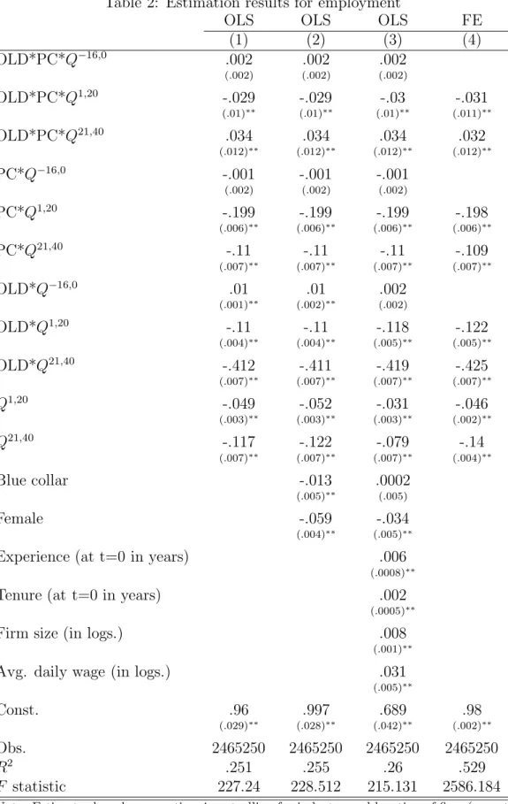
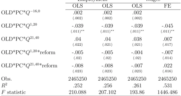
Table 2 presents results in which the outcome variable Yi,t is a dummy
indicating an individual’s employment status at quarter t. Column (1) re-ports the results from a simple OLS regression (a linear probability model) corresponding to the specification described in equation (4). To interpret these estimates correctly let us calculate, as an example, the employment probability of a non-displaced prime-age worker before plant closure. In that case all dummy variables are equal to zero, so the constant term measures this probability. For the non-displaced prime-age workers, employment rates change over time. During the first five years after the (hypothetical) plant closure date employment rates are 4.9 points lower than before (see the row for Q1i,t,20), and during years 5 to 10 after the plant closure date, employment rates are 11.7 points lower than before the plant closure date (Q21i,t,40). This reduction in employment rates is - together with the (full)-employment re-striction in the construction of the data set - the result of aging. On average workers are 9.5 years older during quarters 21 to 40 as compared to during quarters -16 to 0 and this increase in age is most likely the dominant force behind the reduction in employment rates.
Consider next the cohort effect on employment rates of non-displaced workers. As indicated by the coefficientsOLD∗Ql,uin Table 2, workers who
are between age 45 and 55 at the date of plant closure (for whom OLD∗Ql,u
= 1) are only 1 percentage point less likely to be employed in the four years before plant closure than workers who are between age 35 and 44 years at the date of plant closure (see coefficientOLD∗Q−16,0). However, this difference widens to 11 points during the five years following plant closure, and increases dramatically to 41.2 points during the quarters 21 to 40 after plant closure. This increasing gap clearly reflects a life-cycle effect as older workers start to leave the labor force and they increasingly do so as they grow older.13
Now compare displaced workers to non-displaced workers. The coeffi-cients of the interaction P C ∗Ql,u show that, before the plant closure date
these two groups are equally likely to be found in employment. However, after plant closure there are large and highly persistent differences in em-ployment probabilities of these two groups. During the first five years after the date of plant closure, displaced workers have an almost 20 (!) percentage points lower employment rate than non-displaced workers. Even six to ten years after the plant closure date, the difference in employment rates between these two groups amounts to more than 10 percentage points.14
We are now able to discuss the question of our primary interest: Do displaced older workers face significantly worse employment prospects af-ter a job loss than prime-age workers? The coefficients of the inaf-teraction
OLD∗P C∗Ql,u give an answer to this question. Before plant closure there
is no significant additional effect that goes beyond the isolated effects of dis-placement (P C) and age at date of plant closure (OLD) discussed above. This has to be expected because of the almost perfect matching between treated and controls: there should be no pre plant-closure difference. The interaction effect relating to the first five years after displacement indicates significantly lower job chances of older workers after job loss. Workers aged 45-55 at the date of plant closure face an employment rate that is 2.9 per-centage points lower than the one implied by the isolated effect of age at plant closure plus the isolated effect of displacement status.
However, this employment rate penalty does not persist over time. In fact, during years six to ten after plant closure the absolute difference be-tween plant-closure and non-plant closure workers is turned on its head once we account for the interaction effect of age at plant closure and displacement status. Workers aged 45-55 at the date of plant closure now face an employ-ment rate that is 3.4 percentage points higher than the one implied by the isolated effects of age at plant closure plus the isolated effect of displacement
calendar-time trend – when older workers take advantage of early retirement to a larger extent – which is what happened in Austria during the period under consideration
14Chan and Stevens (2001) find for the U.S. that employment rates of 55 years old
displaced workers four years after displacement were 20 percentage points lower than the employment rate of a control group.
status.
To check the robustness of the results the other columns in Table 2 add additional control variables. Column 2 includes a blue collar dummy and a fe-male dummy as additional regressors, column 3 also accounts for experience, tenure, previous wage and employer size at the plant closure date. All ad-ditionally included variables turn out highly significant with expected signs. However, the coefficients of the age, plant-closure, and quarter-indicators (and their interactions) change only slightly. In particular, the estimated effect of age on job loss due to plant closure is exactly the same as the effect estimated in column 1. As a final robustness check, we allowed for indi-vidual fixed effects in the regression (column 4 of Table 2).15 Interestingly,
even accounting for individual fixed effects leaves the point estimates of the age effects due to plant closure unchanged! Also the remaining coefficients remain very close to the simple model.
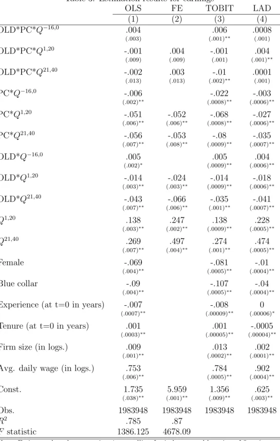
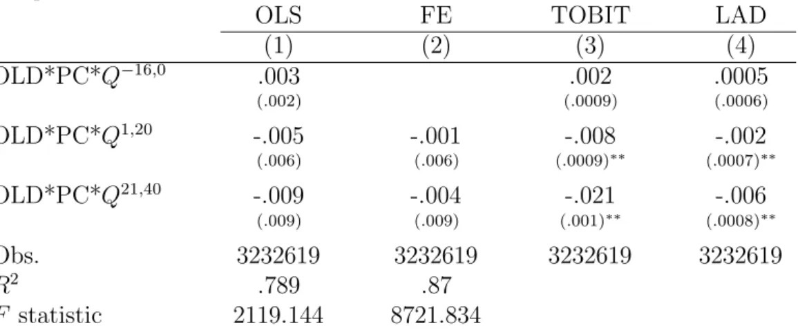
Table 3 presents results from an analogous difference-in-difference regres-sion on earnings. The empirical specification is identical to the above equa-tion but now with the individual’s daily log earnings as the dependent vari-able. In column 1 we estimate a wage equation that includes the full set of variables.16 It turns out that additional earnings losses following plant
clo-sure that are directly caused by age do not exist. All differences-in-differences coefficients are insignificant and negligible in size. Displaced older workers suffer from the same earnings reduction as displaced prime-age workers. How-ever, for all age groups, wage losses are sizable: displacement due to plant closure is followed by a wage reduction of more than 5 percent in the short run and even slightly more in the longer term.17
The remaining coefficients in column 1 of Table 3 are as expected. We see that age at plant closure has a negative effect on earnings growth (as indicated by the negative coefficient of OLD∗Ql,u). Note also that nominal
15In this case an individual fixed effect ν
i is added to the specification in equation
(4), while time-invariant controls, which include all the variables related to the pre-displacement period, are omitted.
16Note that only observations with positive wages are included
17Jacobson et al. (1993) report persistent wage losses of some 30 percent for displaced
workers in the U.S., whereas Ruhm (1991) and Stevens (1997) found somewhat smaller effects. These effects were found for more-tenured workers of all age groups.
daily earnings grew considerably over the observation period. Female workers earn significantly less than male workers and blue collars earn less than white collars. More work experience at the date of plant closure is associated with lower earnings which may be caused by measurement error as experience is left censored in 1972 and wages are top coded or simply by the fact that older workers are already in the declining part of the experience-wage profile. It may also be due to the fact that we include the previous wage as a regressor which may in part capture the positive effect of experience. Tenure, however, has the expected positive impact on the wage. Larger firms pay better and a higher wage at the plant closure date (as a proxy for skills) is associated with higher wages at other dates.
It is also interesting to note that the earnings regression of column 1 has a very high explanatory power: Almost 80 percent of the variance in wages is explained by the variables included in this regression. Controlling for individual fixed effects changes the results only slightly (column 2 of Table 3). In particular, also in the fixed effects estimation, older workers do not suffer from disproportionate earnings losses after displacement. While these losses remain large and statistically significant (both in the short- and in the long-run), prime-age workers and older workers face earnings losses of very similar magnitude. The same picture remains once we run a Tobit regression (accounting for top-coding in earnings data) and when we use the LAD as a robust estimator. Also with respect to other control variables, our estimates remain highly robust and do not seem to be strongly affected by the estimation methods or the inclusion of control variables.
There is only one important difference in the Tobit specification that is worth noting. When top-coding is appropriately taken care of by this specification, old workers seem to experience a statistically significant wage drop in the second five year period (see the third line of column 3 in Table 3). Inasmuch as a drop of reservation wages is more likely to occur for workers who are further away from contractual minima but also more likely to be top-coded in our data, this trend could not be detected by the other specifications of this table and has to be considered for a proper interpretation of the entire evidence.
5
Discussion and robustness checks
Our results can be summarized as follows:
1. Immediately after a plant closure, the old have lower employment prob-abilities than the young.
2. With the passage of time, the old catch up and their employment prob-ability becomes larger than the one of the young.
3. Immediately after plant closure the earnings losses of the young and of the old with respect to the non-displaced are basically identical (ap-proximately 5% in both cases).
4. With the passage of time there is some indication, particularly when the top-coding of wages is properly taken into account by the Tobit specification, that the old who find a new job lose more in terms of wages with respect to the non-displaced than the young in the same condition.
We now study the robustness of these results and discuss some alternative interpretations.
5.1
Data and model specification
One may first worry about the arbitrariness of the definition of young and old. So far a worker was defined as old if her age was greater or equal than 45. In Table 4 we explore a finer classification of workers with respect to age. This table presents estimates of the difference-in-difference parameters
αu,lin equation 4, in which the dummy OLDi has been substituted by three
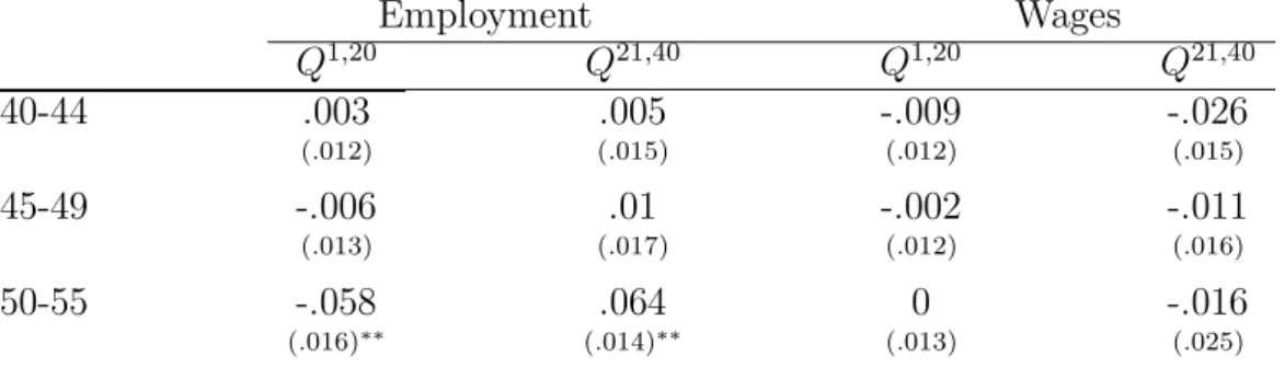
dummies for the age groups 40-44, 45-49 and 50-55, relative to the reference group of 35-39 years old. The first set of estimates, based on all workers, show that all the action comes from the oldest age group. The 50-55 years old are the only ones that really suffer in term of employment in the first 5 years after plant closure (relative to employment losses of displaced workers 35-39 years of age). But there is also clear evidence that they catch up and
improve relative to the younger cohorts in the following 5 years, which for them are the last ones before retirement. In terms of wages, while for this age group there are no signs of wage concessions in the first 5 years after plant closure, a negative albeit insignificant estimate of the difference-in-difference parameter is obtained for the following period, which is consistent with our suggested interpretation of the evidence.
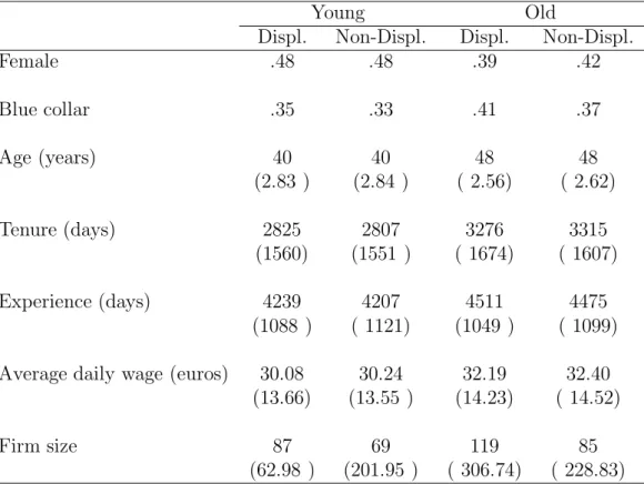
It could be argued that the results described so far are simply driven by a composition effect. At the moment of plant closure the two samples of dis-placed and non-disdis-placed workers are matched according to observables and therefore their composition is very similar. But, later on, death, disabilities and retirement decisions may change the composition of the two samples in different ways, which might explain the pattern of observed result. This pos-sibility, however, is not supported by the evidence displayed in Table 5 which reports the sample averages, by age group and displacement status, of the pre-plant closure characteristics of the workers who are observed with posi-tive wages 5 to 10 years after plant closure. In each cohort, the “left-over” displaced and non-displaced workers appear to be pretty similar on average, suggesting that attrition has not affected in different ways the composition of the two samples in terms of observables.
Another possible interpretation of the evidence is that it results from a non-random selection of the displacement sample. Our definition of dis-placement includes all workers who stayed with their employer until the last quarter before the firm went bankrupt. If workers anticipate the plant’s shut-down, they will search for a new job early on. Under such circumstances, our definition of displacement might produce a negative selection of workers as only the least successful workers will be included in the displaced worker sample. This may not only cause a bias in our estimate of the consequences of plant closure, but it may also affect the implications of age on workers’ job prospects and post-displacement earnings. This problem has been analysed, within the same dataset, by Schwerdt (2007) who suggests, as a robustness check, to include in the set of displaced workers also the “early leavers”. iden-tified as workers who left the plant closure firm during the last half-a-year prior to the plant closure date (between quarters -2 and -1). The implicit
assumption, supported by the statistical analysis of Schwerdt (2007), is that the information that the firm may go bankrupt is revealed within the last half a year prior to bankruptcy. Table 6 presents the results based on this enlarged sample.
Including early leavers in the definition of displaced workers does not change our main result: During the five years following the plant closure date, older displaced workers suffer from a reduction in the employment prob-ability which is almost 3 percentage points larger than the reduction in the employment probability of prime-age workers, relative to the non-displaced in the respective cohorts. During years six to ten following the plant closure date this picture is turned on its head with a more than 3 percentage points lower reduction in employment probabilities for displaced older workers as compared to displaced prime-age workers, again relative to the non-displaced in the respective cohorts. Hence, just like in the baseline model, we conclude that older workers suffer from worse employment prospects than prime-age workers but this loss fades away with the passage of time from plant closure. Table 7 presents results concerning age effects on post-displacement earn-ings when early leavers are included in the displacement sample. Older work-ers suffer from very similar earnings losses after displacement than prime-age workers, both over the short term and the longer term. The point-estimates of the age-specific differences are quantitatively very small and statistically insignificant. Moreover, this result turns out rather robust and holds also in the fixed effect estimation and the Tobit estimation. While the LAD es-timator indicates significantly higher losses for older workers, also here the estimated differences are negligible and amount to only 0.2 percent in the short run and 0.6 percent in the long run. In sum, we conclude that antici-pation of job loss by early leavers is unlikely to lead to major biases in our baseline estimates.
5.2
The role of institutions
In addition to the concerns discussed above regarding the data and the model specification, the role of institutions needs to be examined as well. In
par-ticular one might be worried about retirement regulations as most of the observed decline in employment rates for the older cohort is presumably driven by early retirement. By construction this particular option to with-draw from the labor force is relevant only for the older cohort. However, our identification strategy solely relies on the non-displaced being the counter-factual of the displaced workers at any age. This assumption remains correct inasmuch as retirement possibilities do not differ ex ante (i.e. before plant closure) for the displaced and the non-displaced old. In Austria eligibility for early retirement depends primarily on gender and work experience, while retirement payments are determined mainly by previous earnings. As we match on gender and daily wages and given the insignificant experience dif-ferential between the displaced and non-displaced old, we are confident that our identification assumption is not affected by the retirement system.
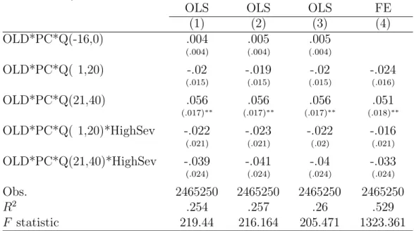
Advance notice legislation and severance payments are also likely to af-fect post-displacement outcomes, as suggested by Card et al. (2006). These factors potentially influence our results insofar as they affect the young and the old differently. In the Austrian case advance notice periods and severance payments vary primarily according to tenure.18 While advance notice periods are rather short in Austria, severance payments are quite generous. Hence, given that older workers are presumably associated with higher tenure, the old displaced have a larger income effect at displacement as opposed to the young displaced. This could affect future labor supply decisions of the two cohorts differently and, specifically, explain the larger employment loss of older workers immediately after displacement, relative to the non displaced. Table 8 presents the results from the estimation of equation 4 for em-ployment, including a fourth difference covering the change in the eligibility for severance payments in the two cohorts. A dummy indicating whether an individual is eligible for above median severance payments is included in the regression together with all relevant interactions. Table 8 reveals that accounting for differences in severance payments, raises the estimates for the difference-in-difference parameters in both post-displacement periods. In the
18See OECD (1993) for an overview of advance notice and severance payments
first 5–year period the effect remains negative, but looses significance. This result is in line with the interpretation that a higher positive income shock at displacement induces older workers to search less intensively for a new job. Hence, the higher loss in terms of future employment probabilities of the old relative to the young can partly be related to differences in severance payments. In other words, the evidence suggests that if severance payments did not increase with tenure, we would not see larger employment losses for the displaced old than for the displaced young, relative to the non displaced. Note, that top-coding in our tenure variable prevents a more explicit analysis of the effect of severance payment eligibility.19
A further potential explanation of the results in the baseline model comes from changes in unemployment insurance rules during the period under con-sideration. Before August 1989, an unemployed person could draw regular unemployment benefits for a maximum period of 30 weeks provided that he or she had satisfied a minimum requirement of previous insurance contributions. In August 1989 the maximum benefit duration was increased to 39 weeks for the age group 40-49 and to 52 weeks for the age group 50 and older.20 This might lead to biases in our estimation results in the employment regressions. More generous unemployment insurance rules for older workers might lead to an increase in the likelihood of being found out of employment. If a job loss destabilizes a worker’s future career, displaced workers are found more often out of employment than non-displaced workers.
However, being out of employment under more generous unemployment insurance rules might amplify the consequences of job loss. As a result, lower employment probabilities of older displaced workers might, partly, be caused by more generous unemployment insurance rules rather than the job-loss as such. To account for such potential upward biases in the estimated age-specific consequences of job loss, we estimate such effects separately
un-19Tenure is only recorded since 1972, which implies that for some observations we can’t
exactly calculate the amount of severance payments in case of displacement. We can, however, identify whether an individual is eligible for above or below median severance payments.
20For a study that looks at the implications of this policy change on unemployment
der the situation where older workers and prime-age workers are subject to identical unemployment insurance rules; and under the situation where these rules are more generous for older workers. If it is true that more generous unemployment insurance rules reinforce the age-effects of job loss on future employment prospects’ we should see a significant negative effect for older workers that are subject to the more generous rules of the 1989 reform for older workers.
Table 9 presents the results from the estimations which are basically in-cluding a fourth difference covering the social security reform. Accounting for changes in unemployment insurance rules after 1989 does not have an impact on the results. While almost exactly the same age-specific effects of job loss emerge as in the baseline model, both in the short run and in the long run, we do not see any additional effect of this reform on age-specific effects on plant closure. Hence we conclude that our basic estimates are quite robust. There may be several reasons why such additional unemployment-insurance effects do not materialize. First, the plant closures we consider in our sample did occur between 1982 and 1988. This means the unemployment spells that were caused by layoffs due to plant closure were not yet subject to the new unemployment insurance rules. Any effect of the new rules could materialize only through recurrent unemployment at later stages. Our estimates indi-cate that, for any later unemployment spells, the reform affects prime-age workers and older workers to the same extent. A second reason follows from our empirical strategy. Our sample of prime-age workers was based on the criterion that a worker had to be between 35 and 44 years old at the date of plant closure. We then follow workers for the next ten years. However, many of the prime-age workers pass the age 50 threshold (and become eli-gible to a longer potential duration of benefit) during the years after plant closure. This mitigates any possible bias that may result from more generous unemployment insurance rules in the first place (by making the prime-age and older workers better comparable also along the unemployment insurance dimension).
5.3
A suggested behavioral interpretation
With the possible exception of the role of severeance payments, none of the other explanations discussed so far can fully account for the evidence as summarized by the four facts listed at the beginning of Section 5. These four facts can instead be interpreted consistently within the following story.
Immediately after a plant closure the old are considered by the market less productive than the young but do not decrease their reservation wage enough to keep their employment probability in line with the one of the young, relative to the non-displaced. This might be due to the effect of sev-erance payments of which we gave some evidence in Section 5.2.21 This is
Result 1. The catching up that characterizes the old in the long run can instead be explained by their increasing impatience induced by the approx-imation of retirement age and more generally by their increasingly shorter time horizon. The hypothesis here is that the discount rate increases more than proportionally with age.22 Thus, with the passage of time after plant closure both the young and the old get older, but the discount rate (impa-tience) increases more for the old than for the young. This delivers Result 2.
Result 3 says that immediately after plant closure there is no difference in the wage losses of the young and of the old who find a job, with respect to the non displaced. This is consistent with the idea that the old are not making the wage concessions that would be needed to sustain their employability, given a decline in their productivity. But towards the end of the observation period, there is some evidence that the old who find a job lose more in terms of wages than the young with respect to the non-displaced, which is Result 4. The lack of strong statistical significance of the evidence based on wages may cast doubts on the relevance of this interpretation, but it should be noted that in the presence of contractual minimum wages, a drop in the compensation of the re-employed workers is less likely to occur for all those
21See also Card et al. (2006).
22We are not aware of any direct evidence on this hypothesis, which, however, seems
plausible: one day before death the discount rate is close to infinity, abstracting from bequest motives.
workers who are at the bottom of the wage distribution and who can enjoy the advantages of social assistance. Not surprisingly, in fact, we see more evidence of this trend when we take top-coding into account in column 3 of Table 3.
To conclude, both the employment and the wage results support the same story from different perspectives. Immediately after plant closure, the old are considered less productive and are offered lower wages but they are reluctant to make wage concessions in order to find quickly a new job also because of the effect of tenure based severance payments. For these reasons their probability of re-employment is lower in the short run after displacement, relative to the non displaced. In the long run instead, their higher impatience prevails, inducing them to accept larger wage losses in order to find a job before retirement.
6
Conclusion
Older workers are in general characterized by lower employment rates than prime age workers. In this paper we use data for Austria to show that, relative to non displaced workers of corresponding age, older workers have lower re-employment probabilities immediately after displacement as compared to prime-age workers in the same situation. After five years, instead, the old displaced are able to catch up with the non-displaced of similar age while this does not happen to the young displaced.
We obtained these results with an estimation strategy that combines the advantages of exact matching to improve the comparability of treated and control subjects, with the advantages of differencing in panel data to con-trol for remaining confounders captured by time invariant individual effects, cohort effects and time effects. Our identification assumption is that the counterfactual of the displaced workers at any age, are the (almost exactly matched) non-displaced workers. The causal effect of beeing displaced at an older age as opposed to a younger age is identified by how the difference of the employment profiles of displaced and non-displaced workers change with age.
Our results can be understood as a combination of demand effects that prevail immediately after displacement and supply effects that kick in later. More specifically, these results are consistent with the view that after plant closure older workers are considered less productive by the market but are at the same time reluctant to lower their reservation wages enough to ensure the same employability as the young. This reluctance is likely to be related to the effect of tenure based severance payments. With the passage of time, the shorter time horizon of the old induce them to lower their reservation wage in order to find a job before retiring, and this explains the observed catching up.
We believe that these findings are relevant for the debate on the oppor-tunity of increasing the retirement age in the presence of Pay-As-You-Go pension systems with an aging population. Our evidence suggests that in-creasing the retirement age does not necessarily produce individuals who are “too old to work but too young to retire”.
References
Ahituv, A. and Zeira, J. (2000). Technical progress and early retirement. CEPR Discussion Papers 2614, C.E.P.R. Discussion Papers.
Bartel, A. P. and Sicherman, N. (1993). Technological change and retirement decisions of old workers. Journal of Labor Economics, 11(1):162–183. Card, D., Chetty, R., and Weber, A. (2006). Cash-on-hand and competing
models of intertemporal behavior: New evidence from the labor market. NBER Working Papers 12639, National Bureau of Economic Research, Inc. Forthcoming in Quaterly Journal of Economics.
Card, D. and Sullivan, D. G. (1988). Measuring the effect of subsidized training programs on movements in and out of employment.Econometrica, 56(3):497–530.
Chan, S. and Stevens, A. H. (2001). Job loss and employment patterns of older workers. Journal of Labor Economics, 19(2):484–521.
Daveri, F. and Maliranta, M. (2007). Age, seniority and labour costs: lessons from the finnish it revolution. Economic Policy, 22:117–175.
Fair, R. C. (2004). Estimated physical and cognitive aging effects. Cowles Foundation Discussion Papers 1495, Cowles Foundation, Yale University. Haltiwanger, John, J. L. and Spletzer, J. (1999). Productivity differences
across employers. the roles of employer size, age and human capital. Amer-ican Economic Review, 89(2):94–98. Papers and Proceedings.
Hellerstein, J. K. and Neumark, D. (2004). Production function and wage equation estimation with heterogeneous labor: Evidence from a new matched employer-employee data set. NBER Working Papers 10325, Na-tional Bureau of Economic Research, Inc.
Hofer, H. and Winter-Ebmer, R. (2003). Longitudinal data from social secu-rity records in Austria. Schmollers Jahrbuch, 123:587–591.
Jacobson, L. S., LaLonde, R. J., and Sullivan, D. G. (1993). Earnings losses of displaced workers. American Economic Review, 83(4):685–709.
Kuhn, P. (2002). Summary and synthesis. In Kuhn, P., editor, Losing Work, Moving On: Worker Displacement in International Perspective. Kalama-zoo, Mich.
Lalive, R., Ours, J. V., and Zweim¨uller, J. (2006). How changes in finan-cial incentives affect the duration of unemployment. Review of Economic Studies, 73(4):1009–1038.
Lazear, E. (1979). Why is there mandatory retirement? Journal of Political Economy, 87(6):1261–1284.
OECD (1993). Long-term unemployment: Selected causes and remedies. In
Employment, Outlook, chapter 3, pages 83–117. Paris. OECD (2005). Aging and employment policies. Paris.
Oster, S. and Hamermesh, D. (1998). Aging and productivity among economists. The Review of Economics and Statistics, 80(1):154–156. Ruhm, C. J. (1991). Are workers permanently scarred by job displacements?
American Economic Review, 81(1):319–324.
Schwerdt, G. (2007). Labor turnover before plant closure: ’leaving the sinking ship’ vs. ’captain throwing ballast overboard’. Ph.d. dissertation - chapter 2, European University Institute.
Skirbekk, V. (2004). Age and individual productivity: A literature sur-vey. Vienna Yearbook of Population Research, pages 133–154. Austrian Academy of Sciences, Vienna.
Stephan, P. E. and Levin, S. G. (1988). Measures of scientific output and the age-productivity relationship. In Raan, A. V., editor, Handbook of Quantitative Studies of Science and Technology, pages 31–80. Elsevier. Stevens, A. H. (1997). Persistent effects of job displacement: The importance
Tables & Figures
Table 1: Descriptive Statistics by displacement status and cohort
“Y oung” “Old”
displ non-displ displ non-displ
Female .49 .49 .48 .48 Blue collar .33 .33 .42 .42 Age (years) 40 40 49 49 (2.8) (2.8) (3.2) (3.2) Tenure (days) 2797 2794 3330 3328 (1558) (1550) (1651) (1618) Experience (days) 4205 4192 4502 4485 (1100) (1130) (1021) (1053)
Average daily wage (euros) 29.91 30.09 30.57 30.74
(13.79) (13.57) (13.91) (13.99)
Firm size 85 67 97 100
(263) (198) (256) (256)
Note: Sample averages with standard deviations in parentheses. All variables, except wage and firm size, are measured at the quarter immediately before (potential or actual) plant closure. The average daily wage is in nominal terms and measured 2 years before plant closure. Firm size is measured 3 quarters before plant closure.
Table 2: Estimation results for employment
OLS OLS OLS FE
(1) (2) (3) (4) OLD*PC*Q−16,0 .002 .002 .002 (.002) (.002) (.002) OLD*PC*Q1,20 -.029 -.029 -.03 -.031 (.01)∗∗ (.01)∗∗ (.01)∗∗ (.011)∗∗ OLD*PC*Q21,40 .034 .034 .034 .032 (.012)∗∗ (.012)∗∗ (.012)∗∗ (.012)∗∗ PC*Q−16,0 -.001 -.001 -.001 (.002) (.002) (.002) PC*Q1,20 -.199 -.199 -.199 -.198 (.006)∗∗ (.006)∗∗ (.006)∗∗ (.006)∗∗ PC*Q21,40 -.11 -.11 -.11 -.109 (.007)∗∗ (.007)∗∗ (.007)∗∗ (.007)∗∗ OLD*Q−16,0 .01 .01 .002 (.001)∗∗ (.002)∗∗ (.002) OLD*Q1,20 -.11 -.11 -.118 -.122 (.004)∗∗ (.004)∗∗ (.005)∗∗ (.005)∗∗ OLD*Q21,40 -.412 -.411 -.419 -.425 (.007)∗∗ (.007)∗∗ (.007)∗∗ (.007)∗∗ Q1,20 -.049 -.052 -.031 -.046 (.003)∗∗ (.003)∗∗ (.003)∗∗ (.002)∗∗ Q21,40 -.117 -.122 -.079 -.14 (.007)∗∗ (.007)∗∗ (.007)∗∗ (.004)∗∗ Blue collar -.013 .0002 (.005)∗∗ (.005) Female -.059 -.034 (.004)∗∗ (.005)∗∗
Experience (at t=0 in years) .006
(.0008)∗∗
Tenure (at t=0 in years) .002
(.0005)∗∗
Firm size (in logs.) .008
(.001)∗∗
Avg. daily wage (in logs.) .031
(.005)∗∗ Const. .96 .997 .689 .98 (.029)∗∗ (.028)∗∗ (.042)∗∗ (.002)∗∗ Obs. 2465250 2465250 2465250 2465250 R2 .251 .255 .26 .529 F statistic 227.24 228.512 215.131 2586.184
Note: Estimates based on equation 4 controlling for industry and location of firm (except for the specification with fixed effects which absorb all time invariant observables and unobservables). The dependent variable is a dummy for the employment status of the
Table 3: Estimation results for earnings
OLS FE TOBIT LAD
(1) (2) (3) (4) OLD*PC*Q−16,0 .004 .006 .0008 (.003) (.001)∗∗ (.001) OLD*PC*Q1,20 -.001 .004 -.001 .004 (.009) (.009) (.001) (.001)∗∗ OLD*PC*Q21,40 -.002 .003 -.01 .0001 (.013) (.013) (.002)∗∗ (.001) PC*Q−16,0 -.006 -.022 -.003 (.002)∗∗ (.0008)∗∗ (.0006)∗∗ PC*Q1,20 -.051 -.052 -.068 -.027 (.006)∗∗ (.006)∗∗ (.0008)∗∗ (.0006)∗∗ PC*Q21,40 -.056 -.053 -.08 -.035 (.007)∗∗ (.008)∗∗ (.0009)∗∗ (.0007)∗∗ OLD*Q−16,0 .005 .005 .004 (.002)∗ (.0009)∗∗ (.0006)∗∗ OLD*Q1,20 -.014 -.024 -.014 -.018 (.003)∗∗ (.003)∗∗ (.0009)∗∗ (.0006)∗∗ OLD*Q21,40 -.043 -.066 -.035 -.041 (.007)∗∗ (.006)∗∗ (.001)∗∗ (.0007)∗∗ Q1,20 .138 .247 .138 .228 (.003)∗∗ (.002)∗∗ (.0009)∗∗ (.0005)∗∗ Q21,40 .269 .497 .274 .474 (.007)∗∗ (.004)∗∗ (.001)∗∗ (.0005)∗∗ Female -.069 -.081 -.01 (.004)∗∗ (.0005)∗∗ (.0004)∗∗ Blue collar -.09 -.107 -.04 (.004)∗∗ (.0005)∗∗ (.0004)∗∗
Experience (at t=0 in years) -.007 -.008 0
(.0007)∗∗ (.00009)∗∗ (.00006)∗
Tenure (at t=0 in years) .001 .001 -.0005
(.0003)∗∗ (.00005)∗∗ (.00004)∗∗
Firm size (in logs.) .009 .013 .002
(.001)∗∗ (.0002)∗∗ (.0001)∗∗
Avg. daily wage (in logs.) .753 .784 .902
(.006)∗∗ (.0005)∗∗ (.0004)∗∗ Const. 1.735 5.959 1.356 .625 (.038)∗∗ (.001)∗∗ (.009)∗∗ (.003)∗∗ Obs. 1983948 1983948 1983948 1983948 R2 .785 .87 F statistic 1386.125 4678.09
Note: Estimates based on equation 4 controlling for industry and location of firm (except for the specification with fixed effects which absorb all time invariant observables and unobservables). The dependent variable is the log-wage of the worker. Standard errors in
Table 4: Estimation results for three age groups relative to the 35-39 age group Employment Wages Q1,20 Q21,40 Q1,20 Q21,40 40-44 .003 .005 -.009 -.026 (.012) (.015) (.012) (.015) 45-49 -.006 .01 -.002 -.011 (.013) (.017) (.012) (.016) 50-55 -.058 .064 0 -.016 (.016)∗∗ (.014)∗∗ (.013) (.025) Note: Estimates of the difference-in-difference parameters αl,u based on the fixed effects
specification of equation 4 for three age groups relative to the 35-39 age group. The dependent variable is a dummy for the employment status of the worker. Standard errors in parentheses. All the other coefficients of each regression are omitted to save space.
Table 5: Weighted averages by age group and displacement status for the “left-over” workers
Young Old
Displ. Non-Displ. Displ. Non-Displ.
Female .48 .48 .39 .42 Blue collar .35 .33 .41 .37 Age (years) 40 40 48 48 (2.83 ) (2.84 ) ( 2.56) ( 2.62) Tenure (days) 2825 2807 3276 3315 (1560) (1551 ) ( 1674) ( 1607) Experience (days) 4239 4207 4511 4475 (1088 ) ( 1121) (1049 ) ( 1099)
Average daily wage (euros) 30.08 30.24 32.19 32.40
(13.66) (13.55 ) (14.23) ( 14.52)
Firm size 87 69 119 85
(62.98 ) (201.95 ) ( 306.74) ( 228.83)
Note: Sample averages of the pre-plant closure characteristics, by age group and displace-ment status, for the workers who are observed with positive wages 5 to 10 years after plant closure. All variables, except wage and firm size, are measured at the quarter immediately before (potential or actual) plant closure. The wage is in nominal terms and measured 2 years before plant closure, firmsize is measured 3 quarters before closure. Standard deviations in parentheses.
Table 6: Estimation results for employment including the “early leavers” in the sample
OLS OLS OLS FE
(1) (2) (3) (4) OLD*PC*Q−16,0 .0008 .0008 .001 (.002) (.002) (.002) OLD*PC*Q1,20 -.027 -.027 -.027 -.028 (.008)∗∗ (.008)∗∗ (.008)∗∗ (.008)∗∗ OLD*PC*Q21,40 .032 .032 .032 .031 (.009)∗∗ (.009)∗∗ (.009)∗∗ (.009)∗∗ Obs. 4051446 4051446 4051446 4051446 R2 .266 .27 .275 .532 F statistic 413.163 418.215 392.225 5093.412
Note: Estimates of the difference-in-difference parametersαu,l based on equation 4 for the
“early leavers” sample. Specifications as in the corresponding columns of Table 2. The dependent variable is a dummy for the employment status of the worker. Standard errors in parentheses. All the other coefficients of each regression are omitted to save space.
Table 7: Estimation results for earnings including the “early leavers” in the sample
OLS FE TOBIT LAD
(1) (2) (3) (4) OLD*PC*Q−16,0 .003 .002 .0005 (.002) (.0009) (.0