Determinacy for infinite games with more
than two players with preferences
Benedikt L¨owe
Institute for Logic, Language and Computation, Universiteit van Amsterdam, Plantage Muidergracht 24, 1018 TV Amsterdam, The Netherlands,
Abstract
We discuss infinite zero-sum perfect-information games with more than two players. They are not determined in the traditional sense, but as soon as you fix a preference function for the players and assume common knowledge of rationality and this preference function among the players, you get determinacy for open and closed payoff sets.
2000 AMS Mathematics Subject Classification.91A06 91A10 03B99 03E99. Keywords. Perfect Information Games, Coalitions, Preferences, Determinacy Ax-ioms, Common Knowledge, Rationality, Gale-Stewart Theorem, Labellings
1 Introduction
The theory of infinite two-player games is connected to the foundations of mathematics. Statements like
“Every infinite two-player game with payoff set in the complexity class Γ is determined, i.e., one of the two players has a winning strategy”
1 The author was partially financed by NWO GrantB 62-584in the project
are called determinacy axioms (for two-player games). When we sup-plement the standard (Zermelo-Fraenkel) axiom system for mathematics with determinacy axioms, we get a surprisingly fine calibration of very interesting logical systems. Research in set theory from the 1960es to this day has shown that many if not most of the interesting features of Higher Set Theory are con-nected to determinacy axioms for two-player games: they have connections to infinitary combinatorics of large sets, to topology, to the theory of the real numbers, and to many other areas of interest in foundations of mathematics. In general, determinacy axioms provide a rich theory of interesting features. (Cf.[Ka94, §§27–32].)
A natural but na¨ıve approach would be to assume that if you increase the number of players and look at “determinacy axioms for three-player games”, the number of interesting features for set theory should also increase. It is well-known that the opposite is true: determinacy axioms of the above form for
n-player games are only interesting if n= 2. In all other cases, they are trivial: Ifn= 1 they are all true, regardless of Γ, if n >2 they are all false for almost all Γ (cf.Proposition 1). It turns out that if we want to give solution concepts for infinite many-player games, determinacy in the classical sense is not the right concept. Solutions that have been offered in the literature include giving up the notion of a pure strategy and moving to mixed strategies (cf. [Ga53] and [Br00]), and understanding many-player games as coalitional games. In this paper, we want to work with pure strategies and stay within the realm of non-cooperative perfect information games
In addition to common knowledge of rationality of all players involved, we need to add fixed preferences of the players and common knowledge of these preferences. Then we are able to give solution concepts for many-player infinite games (for payoffs of very restricted complexity, though).
The results of this paper are (for definitions, cf.Sections 2 and 3):
LetIbe an arbitrary set of players,X an arbitrary set of moves,µan arbitrary moving function, Π an arbitrary total preference.
• If P is an open or closed payoff, then there is a rational labelling `∗ such
that one of the players has an SΠ
`∗-winning strategy. (Theorems 8 and 9) • IfhP,Πiis a exceptional least evil situation, then there is a rational labelling
`∗ such that one of the players has anSΠ
`∗-winning strategy. (Theorem 13) • IfP is a payoff such that a finite set of players has a closed payoff set and the
rest of the players have an open payoff set, then there is a rational labelling
`∗ such that one of the players has an SΠ
`∗-winning strategy. (Theorem 19)1 1 Theorem 13 is a special case of Theorem 19, but uses a different technique, and
2 Definitions & Motivation
In this paper, we will look at a very general form of infinite zero-sum non-cooperative perfect information games. We have an arbitrary set I of players for this game. Our games will be games of length ω with a set X of possible moves.2 We denote the set of finite sequences of elements of X by X<ω. The
length of a finite sequence p ∈ X<ω will be denoted by lh(p), and we write
hx0x1x2. . . xni for a finite sequence of length n+ 1. Note that X<ω is a tree
ordered by inclusion. Runs of the game are infinite sequences of elements from
X, and we denote that set by Xω. If x = hx
k; k ∈ ωi ∈ Xω, we denote by
x¹m :=hx0x1. . . xm−1i itsrestriction to m.
We have a function µ : X<ω → I called the moving function determining
which player has to move in some position p ∈ X<ω. The set M
i := {p ∈
X<ω; µ(p) =i} is the set of positions where player i has to move.
The branches through X<ω, i.e., the elements of Xω will be partitioned by a
payoff function
P :Xω →I
into the payoff sets for the players. For each i ∈ I, we interpret Pi :=
{x; p(x) = i} to be the set of all those ω-sequences of moves that result in a win for player i.
Since we are dealing with perfect information games, all functionsσi :=Mi →
X will be called i-strategies (that means a player has access to the entire game played so far when making his decision about what to play in a position
p). We call a sequence of strategies~σ =hσi; i∈Iia µ-frame (or justframe
if µ is implicitly determined) if for each i ∈ I, σi is an i-strategy. Clearly, a
µ-frame determines a unique element of Xω by letting the strategies in~σ play
against each other, and we call it z~σ.
Our choice of payoff functions of the type P : Xω → I affects our language:
if a µ-frame~σ is a Nash equilibrium in the usual sense, and P(z~σ) =i, this means that while all players locally optimize their outcome, for all players
j with j 6= i this optimal outcome is still a loss. Consequently, the game-theoretically central notion of a Nash equilibrium becomes a bit stale, and we choose the notion of awinning strategy over the notion of anequilibrium
to be central for this paper. We shall briefly discuss the translation of our determinacy theorems into the language of equilibria after Theorem 8.
2 We are basically working in set theory without the Axiom of Choice, so we would
likeXto be well-orderable (the standard example would be either a finite set X or
X = ω), or at least ACX(X), i.e., the existence of choice functions for X-indexed
A proper analysis of a class C of games would be something like the following theorem scheme:
For each payoff P ∈ C there is some player i ∈ I and an i-strategy σ such that for all relevantµ-frames~τ with τi =σ, we have P(z~τ) = i.
The meaning of “relevant” has to be determined by the game analysis. In the classical two-player case of set theory mentioned above, we have the degenerate case where all strategies are relevant. This yields winning strategies: σ is
winningin the game with payoffP if for everyµ-frame~τwithτi =σ, we have
P(z~τ) = i. As usual, we call a payoff P determined if there is a winning
i-strategy for some i ∈ I. For games with more than two players, winning strategies might not always exist (Proposition 1).
For our classes Γ of payoffs we use the usual complexity classes of descriptive set theory: Xω is endowed with a natural topology (the product topology of
the discrete topology on X), and if X is finite or countable, this is a Polish space. We have the usual pointclasses of open, closed, Borel, projective sets onXω, and for a pointclass Γ, we say that the payoff P :Xω →I is a Γ-payoff
if for all i, Pi ∈Γ.3
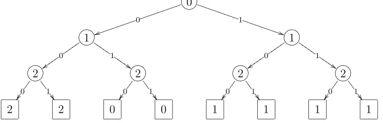
Proposition 1 There is an open three-player game that is not determined.
Proof. Let X :={0,1}, I = 3 ={0,1,2}, µ(p) := lh(p) mod 3 and
P0 :={x; h010i ⊆x orh011i ⊆x},
P1 :={x; h101i ⊆x or h100i ⊆x orh110i ⊆x or h111i ⊆x}, and P2 :={x; h000i ⊆x orh001i ⊆x},
as depicted in Figure 1 or (simplified) in Figure 2.
Clearly, the payoff sets are all open. Figure 2 shows that none of the three
players can have a winning strategy. q.e.d.
Consequently, for games with more than two players, we have to specify a smaller class of strategies as “relevant” in the sense of the above theorem scheme. This is well-known in game theory and led to studying many-player games in terms of coalitions.
As mentioned, we shall stay within the non-cooperative paradigm, but add information about the preferences of the players and their rationality to the
3 Note that this usage is slightly different from the usage in the two-player case. A
?>=<
89:;
00jjjjjj jjj
u
u
jjjjjj
jjj TT1
T T T T T T T ) ) T T T T T T T T T
?>=<
89:;
1 0uuu uu z z uuuuu 1 I I I I I $ $ I I I I I?>=<
89:;
1 0uuu uu z z uuuuu 1 I I I I I $ $ I I I I I?>=<
89:;
2 0©© ¥ ¥ ©© 1 6 6 ½ ½ 6 6?>=<
89:;
2 0©© ¥ ¥ ©© 1 6 6 ½ ½ 6 6?>=<
89:;
2 0©© ¥ ¥ ©© 1 6 6 ½ ½ 6 6?>=<
89:;
2 0©© ¥ ¥ ©© 1 6 6 ½ ½ 6 6 [image:5.612.95.488.30.156.2]2 2 0 0 1 1 1 1
Fig. 1. The game graph of the game from Proposition 1. Round nodes with an i
represent opportunities for player i to move, square nodes denote the winner of a given game path.
?>=<
89:;
00pppppp pp
w
w
pppppp
pp K1
K K K K K % % K K K K K K
?>=<
89:;
1 0¡¡ ¡¡ ¡ ¡ ¡¡¡ 1 > > > > Á Á > > > 1 2 0Fig. 2. Simplified version of Figure 1 with all irrelevant moves removed.
analysis. We shall presuppose full rationality of all players and common knowl-edge of that fact. This allows us to use the usualbackwards induction tech-niques known from perfect information game analysis.4 Assuming common
knowledge of rationality, we can restrict the set of relevant strategies; this will be done when we define the notion of ahΠ, `i-strategy in Section 3.
As an example, consider the game defined in Figure 1 and imagine that we have the three players Jill (0), her husband Jeff (1), and an invited friend John (2). If Jill knows for sure that Jeff prefers her over John, she can exclude his strategy “play 0” from her considerations as irrelevant, and win by playing 0 herself.
Note that this is not a coalition: there is no agreement between Jill and Jeff, there isn’t even a benefit for Jeff. It is just calculation of Jill, taking into ac-count predictions about the behaviour of her husband. Also note that playing 0 can only guarantee Jill to win if she can be sure of both Jeff’s preference for
4 Cf. [Au95], [Bi88], [St96]. For a discussion of the rˆole of common knowledge of
[image:5.612.179.397.211.316.2]her and Jeff’s rationality. If Jeff prefers Jill over John, but doesn’t properly understand what’s going on in the game, he might play 0 and thus let John win. (This type of the game will show up later in Section 7 as Evening at a Couple.)
3 Games with a preference
We call a function Π apartial preferenceif its domain is the setI, and Π(i) is a well-founded partial order on the setI — we also write<i
Π for this partial
order; the intended interpretation of j0 <iΠ j1 is: “player i prefers a win of j0
over a win of j1”. We call a partial preference Π a (total) preference if for
each i ∈ I, Π(i) is a wellordering. In the following, we shall always assume that players want to win,i.e., that
min
<i
Π
I =i
for all i∈I.
Let us define Π0 as follows:
i0 <iΠ0 i1 ⇐⇒ i0 =i & i1 6=i.
Then Π0 is a partial preference that corresponds to the classical zero-sum
situation: all players prefer to win, but if they don’t, they have no prefer-ences about the actual winner. Note that Proposition 1 shows that there is no solution for games with the partial preference Π0.
In the following, we will offer a backwards induction solution concept for infinite many-player games based on a (total) preference that is commonly known. As in the usual situation for infinite perfect information games, we assume that all players are fully rational, and their rationality is common knowledge.
LetI be an arbitrary set of players, µa move function, and Π a total prefer-ence. We call any partial function` :X<ω →I an(partial) labelling.
For each partial labelling` and a total preference Π, we can define its Gale-Stewart procedure in a transfinite recursion as follows:
Start of the recursion and the successor step. We let GSΠ0(`) := `. Suppose that GSΠα(`) is already defined, we then define GSΠα+1(`) as follows:
for each s ∈ X<ω, we check whether one of the cases (s+) or (s−) holds. If
• (s+) Ifµ(s) =i and there is an immediate successor t of s such that
GSΠα(`)(t) =i,
then we let GSΠα+1(`)(s) := i.
• (s−) If µ(s) = i and all immediate successors ofs are already labelled, let
GSΠα+1(`)(s) := min
<i
Π
{j ∈I; ∃ξ∈X(GSΠα(`)(sahξi) = j)}.
If none of the conditions (s+) or (s−) hold, we let GSΠα+1(`)(s) := GSΠα(`)(s)
(which might be undefined).
In words: We interpret a label `(s) = j as “at s it is determined that player
j will win”. If player i has to play at s, the case (s+) means that there is an immediate successor nodet of s such that “at t it is determined that playeri
will win”. Assuming rationality of player i, and assuming that player i wants to win (note that we demanded that of our preferences), this means that “at
s it is determined that player i will win”, since player i will play into such a successor node. The case (s−) means that in all of the successor nodes, the game is determined. In that case, playerican look at the possible labels of the successor nodes, pick the one that he likes best (according to his preference relation <i
Π), and play a successor with such a label. Again, assuming the
rationality of player i and knowledge of the preference Π, the outcome of the game is determined ats.
Note that in general, the Gale-Stewart procedure is non-monotonic: both (s+) and (s−) are able to change labels of GSΠα(`), and so there needn’t be a fixed point. The key idea of Gale and Stewart was that for nice labellings `, the Gale-Stewart procedure is monotonic, and we have a fixed point. In Section 5, we shall see an example where we can do a game analysis even if the procedure isn’t fully monotonic.
The limit step of the recursion. The possibility of non-monotonicity also causes potential trouble with the limit case. In the spirit of Herzberger’s limit rule for the Revision Theory of Truth5 we define
GSΠλ(`)(s) :=
GSΠα(`)(s) if∀β(α≤β < λ → GSΠα(`)(s) = GSΠβ(`)(s)),
undefined otherwise.
Of course, if the procedure is monotonic belowλ, this is the same as the usual definition GSΠλ(`) :=
S
α<λGSΠα(`).
Ifηis a fixed point of the Gale-Stewart construction,i.e., GSΠη(`) = GSΠη+1(`), we call GSΠη(`) the Gale-Stewart closure of ` relative to Π and denote it by GSCΠ(`). Regardless of whether the Gale-Stewart procedure has a fixed point or not, we call the least α such that GSΠα(`)(s) is defined theindex of
s.
Special properties of labellings. Let ` be a partial labelling, Π a total preference, and
hGSΠα(`) ;α ∈Ordi
be the Gale-Stewart procedure starting from `.
We say that ` has the antichain property if for each infinite sequence
hsn;n ∈ Ni with sn+1 % sn there is some n such that sn ∈ dom(`). Note
that this implies that dom(`) is a maximal antichain in X<ω (and for the
labellings` discussed in this paper, it is actually equivalent).
We say that`has the Π-fixed point propertyif the Gale-Stewart procedure starting from ` relative to Π has a fixed point, i.e., for some α, GSΠα(`) =
GSΠα+1(`).
We say that ` has the Π-monotonicity property if for all α ∈ Ord, if
s∈dom(GSΠα(`)), then
GSΠα(`)(s) = GSΠα+1(`)(s).
Obviously, this implies that the Gale-Stewart procedure is monotonic in the usual sense6, and we get a fixed point by the standard fixed point theorem
for monotonic operators:
Lemma 2 If ` has the Π-monotonicity property, it also has the Π-fixed point property.
For some ` that has the Π-fixed point property, we say that it has the Π -totality property, if GSCΠ(`) is a total function. We say that it has the Π-root property if ∅∈dom(GSCΠ(`)).
Lemma 3 (Totality Lemma) If ` has the antichain property and the Π -monotonicity property, then it has the Π-totality property.
Proof. Suppose that s is not labelled by GSCΠ(`). By (s−), all positions that have only labelled immediate successors are labelled in the Gale-Stewart
6 I.e., for all α < β, we have dom(GSΠ
α(`)) ⊆ dom(GSΠβ(`)) and for s ∈
closure. Consequently, we can define an infinite sequence hsn; n ∈ ωi with
sn $sn+1 starting from s such that for all n∈ω, sn ∈/ dom(GSCΠ(`)).
By the antichain property, there is some m such that sm ∈ dom(`). But the
monotonicity property of ` implies that dom(`) ⊆ dom(GSCΠ(`)) which is a
contradiction. q.e.d.
Special properties of strategies. Let S be some class of strategies, and `
be some labelling. We call a frame~τ =hτj; j ∈IianS-frameif for allj ∈I,
we have τj ∈ S.
We call an i-strategy σ `-S-consequent if for every S-frame ~τ such that
τi =σ, we have that
`(z~τ¹n) = i
for alln ∈ω. We call ani-strategyS-winning if for allS-frames~τandx:=z~τ, we have P(x) =i.
We call a strategyσahΠ, `i-strategyif for allpwithµ(p) = i, if`(pahσ(p)i) = k, thenk is the <i
Π-least element of
{j ∈I;∃x(`(pahxi) =j)}.
We denote the set of hΠ, `i-strategies bySΠ
` .
Heuristics: We again assume that `(s) = j is interpreted as “at s it is deter-mined that player j wins”. Suppose µ(p) = i; using his knowledge about `, player i will be able to check his options at p by looking at the set
{`(pahξi) ;ξ ∈X}.
Given the above interpretation of `, the only rational choice for player i is to choose one of the successors that rank highest in his preference. A hΠ, `i -strategy is one in which the player is required to behave rational in this way.
Lemma 4 Let ` be a labelling with the Π-totality property. Then there is a
GSCΠ(`)-SΠ GSCΠ
(`)-consequent strategy.
Proof.We write`∗ := GSCΠ(`). By the Π-totality property, we have`∗(∅) = i
for some i ∈ I. We define the following i-strategy σ: if µ(p) = i, play some
ξ such that pahξi has the <i
Π-least label among the immediate successors of p. The labelling `∗ is a total function and a fixed point of the Gale-Stewart
procedure, so for each node s, `∗(s) must also be the label of at least one
immediate successor of s.
Fix any SΠ
`∗-frame ~τ such that τi = σ, and let x :=z~τ. We shall show that
counterexample (thus`∗(x¹n) = iand `∗(x¹n+ 1) 6=i). By the above remark,
we know that there is some immediate successorp ofx¹n such that `∗(p) = i.
Thus, by the choice ofσ, we know thatµ(x¹n) =j 6=ibecause playeriwould have chosen to play p instead ofx¹n+ 1. But now by (x¹n−), we have
i= min
<jΠ
{k ∈I; ∃ξ ∈X(`∗(sahξi) =k)},
yet τj(x¹n) = x(n) with i <jΠ `∗(x¹n+ 1). Thus τj is not a hΠ, `∗i-strategy.
Contradiction. q.e.d.
4 Open and Closed Preference Games
4.1 Open Payoffs
Now letIbe an arbitrary set of players,µa move function, Π a total preference, and P an open payoff.
We define
Si :={p∈X<ω; ∀x(p⊆x implies P(x) = i)}
to be the set of positions at which playeri has won, and set
`(p) :=i:⇐⇒ p∈Si.
We call a labelling` anopen labellingif there is an open payoff P as above.
Lemma 5 Every open labelling has the antichain property.
Proof. Obvious. q.e.d.
Lemma 6 Every open labelling has the Π-monotonicity property (for arbi-trary preferences Π).
Proof. Let hGSΠ`(α) ;α ∈ Ordi be the Gale-Stewart procedure derived from
`. We prove the claim by induction on the index of s. Suppose s is a coun-terexample of minimal index, so GSΠα(`)(s) =i6=j = GSΠα+1(`)(s). Take α to
be minimal among those as well.
Case 2. The index is β+ 1, and s was labelled by (s−). Then all immediate successors thave strictly lower index, and thus by minimality, their labels are fixed. So (s−) is applied in the construction of GSΠα+1(`), hence GSΠα+1(`)(s) = i. Contradiction.
Case 3. Suppose that the index of s is 0. In that case, all successors (not only immediate) are i-labelled with index 0, so by induction GSΠα+1(`)(s) = i.
Contradiction. q.e.d.
Corollary 7 Every open labelling has the Π-totality property (for arbitrary preferences Π).
Proof. From Lemmas 5 and 6 via the Totality Lemma 3. q.e.d.
Theorem 8 LetIbe an arbitrary set of players,µan arbitrary move function, P an open payoff, ` the open labelling derived from P, `∗ its Gale-Stewart
closure, and Π a (total) preference. Then there is an i∈I and a SΠ
`∗-winning strategy σ for player i.
Proof. By Corollary 7, GSCΠ(`) is total, so let GSCΠ(`)(∅) =i. Using (the proof of) Lemma 4, we get a GSCΠ(`)-SΠ
`∗-consequent strategyσ for player i.
Let~τ be an arbitrary SΠ
`∗-frame with τi =σ, and let x:=z~τ. We have that
for every n∈ω, GSCΠ(`)(x¹n) =i.
Lemma 5 gives us somem such thatx¹m∈dom(`), and Lemma 6 yields that
`(x¹m) = GSCΠ(`)(x¹m) = i, i.e.,x∈Si, and thus P(x) = i. q.e.d.
In terms of determinacy axioms, the analysis of this section yields a many-player determinacy statement:
For open payoffs and arbitrary sets of players, if we fix a (total) preference Π, then there is a Π-winning strategy for one of the players.
Let us rephrase this in terms of equilibria: If we restrict the class of relevant strategies to the strategies inSΠ
`∗, then Theorem 8 gives us a large set of very
strong equilibria: Each frame~τsuch thatτi =σis an equilibrium since none of
the players can increase his payoff while playing a strategy inSΠ
`∗; the players j 6=i necessarily lose against σ.
4.2 Closed Payoffs
IfI is finite andP is closed, then all setsPi are also open, and Theorem 8 can
clopen. However, a slight modification of the above argument (using closed labellings instead of open labellings) yields the same result:
Let I be an arbitrary set of players, µ a move function, Π a total preference, and P a closed payoff.
We define
Ci :={p∈X<ω; ∀x(p⊆x implies P(x)6=i)}
to be the set of positions where player i has irrevocably lost, and define the labelling
`(s) =i:⇐⇒ ∀j ∈I (j 6=i→s∈Cj).
We call such a labelling anclosed labelling.
Now it’s easy to see closed labellings also have the antichain and the mono-tonicity property. So by the Totality Lemma 3, `∗ = GSCΠ(`) is a total
func-tion. Lemma 4 gives an SΠ
`∗-consequent strategy, which then by definition of `
yields a SΠ
`∗-winning strategy:
Theorem 9 LetIbe an arbitrary set of players,µan arbitrary move function, P a closed payoff, ` the derived closed labelling, `∗ its Gale-Stewart closure,
and Π a (total) preference. Then there is an i∈I and a SΠ
`∗-winning strategy σ for player i.
4.3 Exceptional Least Evil
We shall now briefly discuss a special situation which occurs rather frequently and can be solved with (a variant of) the methods of this section.
If Π is a preference, we say that i0 ∈ I is a least evil in Π, if for all i 6=i0,
we have
i <i
Πi0 <iΠj
for all j /∈ {i, i0}.
We call a pairhP,Πianexceptional least evil situationifi0 is a least evil,
andP is a payoff such thatPi is open for alli6=i0. Clearly, Pi0 is then closed.
Fori6=i0, we define
Si :={p∈X<ω; ∀x(p⊆x implies P(x) = i)}
and
`(p) := i:⇐⇒ p∈Si
We get analogues of Lemmas 5 and 6:
Lemma 10 If hP,Πi is an exceptional least evil situation and ` the derived labelling, then for every x∈Xω, we have
• either there is some n such that x¹n∈dom(`), • or P(x) =i0.
Lemma 11 If hP,Πi is an exceptional least evil situation, then its derived labelling has the Π-monotonicity property.
Consequently, exceptional least evil labellings have the Π-fixed point property. However, the Gale-Stewart closure needn’t be total this time as they do not have the antichain property. We define
`∗(s) =
GSCΠ`(s) if s∈dom(GSCΠ(`)), and
i0 otherwise.
Ifs /∈dom(GSCΠ(`)), we say that the index of s is 0.
Lemma 12 If hP,Πi is an exceptional least evil situation, ` the derived la-belling and `∗ defined as above, then there is an `∗-SΠ
`∗-consequent strategy. Proof. Suppose that `∗(∅) = i. As in the proof of Lemma 4, we define a
strategyσ for player i: ifµ(p) = i, letipmin := min<i
Π{`
∗(pahξi) ; ξ∈X}. Look
at the set Ξp := {ξ ∈ X; `∗(pahξi) = ip
min}. Pick ξ0 from this set such that
the index ofpahξ
0i is minimal. Note that if the index ofpis not zero, there is
some ξ0 ∈Ξp such that the index of pahξ0i is strictly lower than the index of p.
We claim that this strategy is `∗-SΠ
`∗-consequent.
If `∗(∅) =i 6=i
0, this proof is essentially the same as the proof of Lemma 4.
Suppose that `∗(∅) = i
0. Observe that the only way s can be labelled i0 is
if s has an immediate successor that is labelled i0 (otherwise, all immediate
successors have are labelled by GSCΠ(`), and hence alsos itself). Let~τ be an arbitrarySΠ
`∗-frame with τi0 =σ and x:=z~τ. Take n such that `
∗(x¹n) = i
0
and `∗(x¹n + 1) = j 6= i
0. Obviously, µ(x¹n) = k 6= i0. If j = k, then `∗(x¹n) = GSCΠ
`(x¹n) = j by (x¹n+). Consequently, j 6= k. But now we can
use that i0 is the least evil, so in particular, k <kΠi0 <kΠj. But
`∗(x¹n)aτ
k(x¹n)) =j,
soτk is not ahΠ, `∗i-strategy. Contradiction. q.e.d.
func-tion, hP,Πi an exceptional least evil situation, ` the derived labelling, and `∗
as defined above. There is an i∈I and an SΠ
`∗-winning strategyσ for playeri. Proof. The strategy σ as defined in the proof of Lemma 12 will be the SΠ
`∗
-winning strategy. Remember thatσalways plays into positions of strictly lower index (unless the index is 0). Let~τ be a SΠ
`∗-frame with τi =σ and x:=z~τ.
Then by Lemma 12, `∗(x¹n) = i for all n∈ω.
We are left to show that P(x) = i. By Lemma 10, we know that this is the case if i=i0. So leti6=i0.
Note that if µ(x¹n) = j 6= i, then it was either already i-labelled in ` or it wasi-labelled by (x¹n−), so all immediate successors have strictly lower index thanx¹n. This together with the choice ofσ says that the sequence of indices of x¹n is a decreasing sequence of ordinals. Hence it must eventually reach 0,
which means that x¹n ∈Si for some n ∈ω. q.e.d.
The fact that the index function needs to be used in order to define a winning strategy in this case is no coincidence: as opposed to games in which all payoffs are open or all payoffs are closed, the games with an exceptional least evil contain for example all so-calledcombinatorial games(games with counters on graphs; the last player to move the counter wins, if the counter is moved infinitely many times, it’s a draw). That labelling functions for combinatorial games need transfinite ordinal values to describe winning strategies has been discussed in [FrRa01].
5 Mixed Labels
The analysis of Section 4, in particular Section 4.3 covers quite a lot: The usual open and closed two-player games (i.e., P0 open and P1 closed, or vice versa) are an instance of an exceptional least evil (the closed player is the exception); also all games with open payoffs and a draw are instances of an exceptional least evil (as mentioned, the combinatorial games on graphs are examples of these).
But there are other situations that the analysis of Section 4.3 cannot deal with, for example a closed player who is not a least evil, or two closed and one open players.
For these situation we need to mix open and closed labellings, and give up monotonicity.
is either open or closed for all i ∈ I. We shall call such a payoff function a
mixed payoff. Let Iopen∪Iclosed be a disjoint partition of I such that for all i ∈ Iopen, Pi is open and for all i ∈ Iclosed, Pi is closed. Assume in addition
that Iclosed is finite (this is used in the proof of Lemma 14).
We are now joining the ideas of open and closed labellings. For eachi∈Iclosed,
let
Ci :={p∈X<ω; ∀x(p⊆x implies P(x)6=i)}
be the set of positions where playerihas irrevocably lost, and for eachi∈Iopen,
let
Si :={p∈X<ω; ∀x(p⊆x implies P(x) = i)}
be the set of positions at which player i has won.
We define the following mixed labelling:
`(s) :=
i∈Iopen if s∈Si,
j ∈Iclosed if s /∈S{Si; i∈Iopen} ∪S{Ck; k ∈Iclosed, k6=j}.
Labellings derived from a mixed payoff function in this way are called mixed labellings.
Lemma 14 Every mixed labelling has the antichain property.
Proof. Letx ∈Xω, and let P(x) =i. If i ∈I
open, then there is some n such
that x¹n ∈Si.
If i ∈ Iclosed, then for each j ∈ Iclosed such that j 6= i there is some natural
number nj with x¹nj ∈ Cj. Let n := max{nj;j ∈ Iclosed, j 6= i} (note that
this exists becauseIclosed is finite). Then `(x¹n) = i. q.e.d.
If nowhGSΠα(`) ; α∈Ordiis the Gale-Stewart procedure starting from a mixed
labelling `, it is not necessarily monotonic anymore:
For example, ifI =X ={0,1},µ(∅) = 0,P0 :={x; x(0) = 0}, then`(∅) = 1
and `(h0i) = 0. Then (∅+) gives GSΠ1(`)(∅) = 0 6= 1 = GSΠ0(`)(∅). We call such a situation, i.e., a pair hs, αi such that
GSΠα(`)(s) =i=6 j = GSΠα+1(`)(s)
anoverwriting instance (for`).
Lemma 15 If `is a mixed labelling and hs, αi is an overwriting instance with
GSΠα(`)(s) = i6=j = GSΠα+1(`)(s),
Proof. We prove this by induction on the index of s. Suppose s is a coun-terexample of minimal index. Take α to be minimal among those as well.
Case 1., Case 2. and Case 3. from the proof of Lemma 6, show that the index of s must be 0, and that i cannot be an open label, so i ∈ Iclosed. By
definition of `, we know that
Iclosed∩ {`(t) ; t⊇s}={i}.
So by induction, GSΠα(`)(t)∈Iopen∪ {i}for all successorst⊇s. Consequently,
if GSΠα+1(`)(s) =j 6=i, then j ∈Iopen. But now the minimal choice ofα gives `(s) = GSΠα(`)(s) by induction, sos was no counterexample. q.e.d.
Corollary 16 If ` is a mixed labelling and s ∈ X<ω, then there is at most
one α such that GSΠα(`)(s)6= GSΠα+1(`)(s).
Proof. By Lemma 15, if GSΠα(`)(s) 6= GSΠα+1(`)(s), then GSΠα(`)(s) ∈ Iclosed
and GSΠα+1(`)(s)∈Iopen. But now again by Lemma 15 this means that for no β > α, we can have GSΠβ(`)(s)= GS6 Πβ+1(`)(s). q.e.d.
Lemma 17 Every mixed labelling has theΠ-fixed point property (for arbitrary
Π).
Proof. By Corollary 16, there is only a set of overwriting instances (in fact, the cardinality of the set is at mostκ := Card(X<ω). Let
Σ := sup{α+ 1 ; hs, αi is an overwriting instance for some s ∈X<ω}.
Then after Σ, the Gale-Stewart procedure is fully monotonic, and hence has a fixed point by the usual fixed point theorem. q.e.d.
Lemma 18 Every mixed labelling has the Π-totality property (for arbitrary
Π).
Proof. We know by Lemma 14 that ` has the antichain property. Note that the proof of the Totality Lemma 3 doesn’t really need the full Π-monotonicity property but only
s∈dom(`) → s ∈dom(GSCΠ(`)) (†)
which is a consequence of Corollary 16. q.e.d.
Theorem 19 Let I =Iopen∪Iclosed be an arbitrary set of players where Iclosed is finite, µ an arbitrary move function, P a payoff such that Pi is open for
i ∈ Iopen and Pi is closed for i ∈ Iclosed, ` the derived mixed labelling, and `∗
its Gale-Stewart closure (which exists by Lemma 17). Then there is an i∈ I and an SΠ
Proof. By Lemma 18, `∗ is total, so by (the proof of) Lemma 4, we have a
`∗-SΠ
`∗-consequent strategy σ for player i such that `∗(∅) = i.
To prove the theorem, it is enough to show the following:
We show that if x∈Xω such that for alln, `∗(x¹n) =i, then P(x) = i.
Case 1. Leti∈Iopen. By Lemma 14, we get some n such that`(x¹n) =i, so x∈Si, so P(x) = i.
Case 2. Let i ∈ Iclosed. If x ∈ S{Pj; j ∈ Iopen}, then there is some n such
that `(x¹n) ∈ Iopen. But then by Lemma 15, `∗(x¹n) = `(x¹n) ∈ Iopen.
Con-tradiction.
So, we have that x ∈ S
{Pj; j ∈ Iclosed} and by Lemma 14 that for some n, `(x¹n) = i. By definition of the closed labels in `, this means that x /∈ S
{Pj; j ∈Iclosed, j =6 i}, so P(x) = i. q.e.d.
6 Temporal Game Logic
In his [vB03,§8.2], van Benthem discusses the Gale-Stewart theorem in terms of a branching time logic with additional game operators. We think of Xω as
the set of branches in a model for a Prior-style branching time logic with the usual operators G (“for all future times”) and H (“for all past times”), and the derived operator Aϕ≡Gϕ∧Hϕ.7 Motivated by looking at finite games
[vB03, §5.3], van Benthem adds game modalities Wi for each of the players
i∈I with the intended meaning “player i can force”.
If x ∈ Xω and s ∈ X<ω, then the semantics for W
i is hx, si |= Wiϕ if and
only if there is a strategy for player i such that every run of the gamey ⊇ s
consistent withy (beyond s), we get hy, ti |=ϕ for all s ⊆t⊆y.
Considering a two-player situation with an open payoffP0 and a closed payoff P1 where membership inP0 is described byϕ, the key step of the Gale-Stewart
argument transforms into the modal formula
W0ϕ∨W1A¬W0ϕ:
7 For a thorough account of Prior’s tense logics, cf. [M¨u02]; for the original
either player 0 can force the outcome into P0 or player 1 can make sure that
player 0 can never force the outcome into P0.8
This is exactly the claim of Lemma 12, and if we are in the case of the second alternative (W1A¬W0ϕ), we use the fact thatP1 is closed to show that this
is enough to prove that the outcome is in P1.
Of course, when we move to more general formulas ϕ of temporal logic, the Weak Determinacy formula might not be enough to prove determinacy any-more, and also the provability of the Weak Determinacy formula might depend on the system we’re working in.
In the cases of open payoffs, closed payoffs and mixed payoffs with the non-monotone analysis of Section 5, the explication in a temporal game logic term becomes even simpler and is identical with the statement of determinacy:
_
i∈I
Wiϕi
where ϕi is a formula describing membership in Pi.9 The case of the
Excep-tional Least Evil reverts to the Gale-Stewart situation and gives
_
i6=i0
Wiϕi ∨ Wi0A
^
i6=i0
¬Wiϕi.
7 Games with three players
We now give some examples of games solved by the solution concepts by open labellings and mixed labellings given in Sections 4 and 5.
For this let’s look a bit more closely at three-player games with preferences. Up to renaming of the players, there are only two different three-player games with total preferences, we call themEvening at a Married Exand Love Triangle
(depicted in Figure 3). In our pictures of the preferences, an arrow from i to
j means “iprefers j overk” (where {i, j, k}={0,1,2}).
Of course, the solution concept presented in Theorem 19 gives us optimal strategies for some player in these games if the payoffs are open and/or closed.
8 This is calledWeak Determinacy by van Benthem [vB03]. 9 If I is infinite, we either need to interpret the disjunction W
0jj **1 0 **1
w
w
2
V
V
2
V
V
Fig. 3.Evening at a Married Ex andLove Triangle
For three players, if Π(i) is not a wellordering, it is necessarily of the form
i <i
Π j, k where j and k are in no particular ordering. So if Π is not a total
preference, then either one, two, or all three of the relations <i
Π are of this
form. There are (up to renaming) three cases with two wellorderings, and one case each with one and zero wellorderings. They are depicted in Figures 4 and 5.
0 **1
w
w
0jj **1 0
'
'
1
w
w
[image:19.612.122.459.187.241.2]2 2 2
Fig. 4. Beatrice’s Revenge,Evening at a Couple, andLeast Evil
In general, there are no solution concepts for partial preferences. Of course,
Hobbesis just the case of full non-cooperation and as mentioned in Proposition 1, there is no solution for this situation. A notable exception isLeast Evil: In the case where the least evil itself doesn’t move (i.e.,M2 =∅), the “Exceptional
Least Evil” analysis of Section 4.3 is a solution.
Let us briefly describe the different situations by examples:
Love Triangle.This situation is truly pseudo-Shakespearean: Beatrice (0) is the fianc´ee of the poor but handsome Captain Antonio (1). She recently started to question her fianc´e’s character. Faking a family emergency, she pretends to go to the countryside while dressing as a rich wine merchant to check on Antonio’s behaviour. Alas, her suspicions prove to be correct: as soon as she apparently leaves town, Antonio starts a liaison with the beautiful Cressida (2). Beatrice in the rˆole the wine merchant is intent on confronting Antonio with his deeds and invites Antonio and Cressida to play an infinite three-player game. Now the treacherous heart of Cressida abandons poor Antonio for the rich wine merchant (0 <2
Π 1) while the good-hearted Beatrice is full
of pity for Antonio seeing him so deceived by Cressida (1<0
Π 2). Antonio, of
course, doesn’t evaluate the situation correctly: he doesn’t recognize Beatrice, and although he realizes that Cressida has abandoned him, he tries to win her back by preferring her in the game (2<1
Π0).
she gives up favouring Antonio over Cressida.
Evening at a Couple.John (2) visits his friends, the married couple Jeff (1) and Jill (0) at home. They decide to kill some time by playing an infinite three-player game. Although Jeff and Jill are good sports and try to play the game without prejudice, subconsciously, they prefer their marital partner over John (0<1
Π2, 1 <0Π2). John knows that pretty well, and realizes that it makes no
difference whether Jeff or Jill wins.
Evening at a Married Ex. We are in the situation of Evening at a Couple but with an added twist: Jill was the girlfriend of John for a long time while they were in graduate school, and (not unbeknownst to Jill) John is still in love with her (0<2
Π 1).
Least Evil. We are in a Mathematics Department with Professors Smith (0), Johnson (1) and Williams (2) eligible to become the new Chair.10 Smith and
Miller are ambitious administrators and know that the only way to become Dean of the Faculty of Sciences is to become Department Chair. Of course, they also know that if the other one becomes Chair, he will probably use his chance to become Dean, and the position of the Dean will be blocked for at least five if not ten years. Williams is not ambitious at all – both Smith and Miller realize that if Williams were to become Chair, he would never aim at the office of Dean (2 <0
Π 1, 2 <1Π 0). As laid out in the bylaws of the
Mathematics Department, Smith, Johnson and Williams have to engage in an infinite three-player game to determine the next Chair.
Of course, Least Evil is a very common situation. As mentioned, if M2 = ∅,
we end up with a two-player game with draw.
0 **1 0 1
2 2
Fig. 5. Sidekickand Hobbes
Sidekick. Luigi (1) and Paolo (2), two mafia bosses meet to deal with each other, and Luigi brought his faithful follower Giacomo (0). They play an infi-nite game, and whoever wins the game will become Overlord of Crime. Each of them is given a chance of winning that title, but what about the consequences of losing? Clearly, if Paolo wins, he will most probably kill both Luigi and
Giacomo to thwart any opposition forming around them; similarly, he can be sure to be killed for the same reason by either of the others if they win. Luigi has humiliated Giacomo over many years, so Luigi can’t be sure of his future if Giacomo wins. The only one who has a preference is Giacomo: if Luigi wins, he will stay alive –and continue to be humiliated by Luigi–; if Paolo wins, he’ll die (1<0
Π 2).
Hobbes. In this three-player game there are no preferences except that all players wish to win, and if they don’t, they don’t care who does. This type of game is played in the Hobbesian Natural Condition of Mankind:
If any two men desire the same thing, which nevertheless they cannot both enjoy, they become enemies; and in the way to their end (which is principally their own conservation, and sometimes their delectation only) endeavour to destroy or subdue one another. ... Men have no pleasure (but on the contrary a great deal of grief) in keeping company where there is no power able to overawe them all. ... It is manifest that during the time men live without a common power to keep them all in awe, they are in that condition which is called war; and such a war as is of every man against every man (Hobbes, Leviathan XIII).
As pointed out, this situation is the fully non-cooperative situation described in Proposition 1, and thus Π-preference determinacy cannot offer a solution concept for these games.
8 Conclusion
We gave solution concepts for infinite multi-player games with the strongest common knowledge assumptions and for very simple payoffs. Of course, there are many directions to discuss variations of these themes:
More complicated payoffs. As can be made explicit,∆02 payoffs still allow combinatorial labellings, thus it is possible to give a version of backwards induction. That suggests that the arguments from this paper could possibly be extended to ∆02 payoffs.
Other knowledge assumptions. Consider the following version of Love Triangle where Antonio is even less observant: He doesn’t recognize Beatrice, but moreover he also doesn’t realize that Cressida has abandoned him, so in evaluating the game tree, he will evaluate the positions as if 1<2
Π 0 instead of
(the correct) 0 <2
Π 1. Assuming that Beatrice and Cressida know about this
error in judgement of Antonio’s, can we give a solution of the game? What if we allow Antonio to change his mind (and thus the labelling of the game tree in his mind) as soon as he sees that Cressida has betrayed him?11 This
necessarily leads to dynamic models of these games similar to dynamic models for epistemic solutions of finite games (cf. [vB01]).
Proof-theoretic analysis & more non-monotonicity. The existence of winning strategies has been analyzed proof-theoretically in terms of weak sys-tems of second-order arithmetic.12
Deleting and overwriting of labels for games as in the analysis of mixed la-bellings occurs in some proof-theoretic analyses of subsystems of second-order number theory [M¨o03], and in full generality might be connected to games corresponding to the proof-theoretic strength of Gupta-Belnap revision the-ory.13 Thus extending the ideas of Section 5 to labellings with the antichain
property but with truly non-monotonic Gale-Stewart procedures that need to be analysed as revision sequences is an interesting approach to game-theoretic analyses of Revision Theory.
References
[Au95] Robert J.Aumann, Backward Induction and Common Knowledge of Rationality, Games and Economic Behavior 8 (1995), p. 6–19
[BAMaPn83] MordechaiBen-Ari, ZoharManna, AmirPnueli, The temporal logic of branching time,Acta Informatica20 (1983), p. 207–226
[Bi88] Ken Binmore, Modelling Rational Players. Part II, Economics and Philosophy 4 (1988), p. 9-55
[Bo01] Giacomo Bonanno, Branching Time Logic, Perfect Information Games and Backward Induction, Games and Economic Behavior 36 (2001), p. 57–73
11For finite games, this has been considered by Kreps et al. in [Kr+82]. 12Cf.[Ta90], [Ta91], [M¨o03], and in particular the textbook [Si99].
[Br00] RodicaBrˆanzei, On the Determinateness ofn-person games with information energy, Revue Roumaine de Math´ematiques Pures et Appliqu´ees45 (2000), p. 67–76
[dB∞] Boudewijnde Bruin, An Application of Epistemic Logic to Some Questions in Game Theory,typoscript
[FrRa01] Aviezri S.Fraenkel, OferRahat, Infinite cyclic impartial games, Theoretical Computer Science 252 (2001), p. 13–22
[Ga53] DavidGale, A theory ofn-person games with perfect information, Proceedings of the National Academy of Sciences U.S.A. 39 (1953), p. 496–501
[GaSt53] David Gale, Frank M. Stewart, Infinite Games with Perfect Information, in: Harold W. Kuhn, Albert W. Tucker (eds.), Contributions to the Theory of Games II, Princeton 1953 [Annals of Mathematical Studies 28], p. 245–266
[GuBe93] Anil Gupta, Nuel Belnap, The Revision Theory of Truth, Cambridge MA 1993
[Ka94] Akihiro Kanamori, The Higher Infinite, Large Cardinals in Set Theory from Their Beginnings, Berlin 1994 [Perspectives in Mathematical Logic]
[Kr+82] David M.Kreps, Paul Milgrom, John Roberts, Robert Wilson, Rational cooperation in the finitely repeated prisoners’ dilemma, Journal of Economic Theory27 (1982), p. 245–252
[K¨uL¨oM¨oWe∞] Kai-Uwe K¨uhnberger, Benedikt L¨owe, Michael M¨ollerfeld, Philip D.Welch, Comparing inductive and circular definitions: parameters, complexities and games, in preparation
[M¨o03] Michael M¨ollerfeld, Systems of Inductive Definitions, Ph.D. Thesis, Westf¨alische Wilhelms-Universit¨at M¨unster, 2003
[M¨u02] Thomas M¨uller, Arthur Priors Zeitlogik, Mentis Verlag, Paderborn 2002
[Si99] Stephen G.Simpson, Subsystems of second order arithmetic, Berlin 1999 [Perspectives in Mathematical Logic]
[St96] Robert Stalnaker, Knowledge, Belief, and Counterfactual Reasoning in Games, Economics and Philosophy 12 (1996), p. 133–163
[Ta90] Kazuyuki Tanaka, Weak axioms of determinacy and subsystems of analysis I: ∆0
2 games,Zeitschrift f¨ur Mathematische Logik und Grundlagen der Mathematik 36 (1990), p. 481–491
[Th70] Richmond H. Thomason, Indeterminist time and truth-value gaps, Theoria36 (1970), p. 264–281
[vB01] Johan van Benthem, Games in dynamic-epistemic logic, Bulletin of Economic Research 53 (2001), p. 219–248