Review
Quantitative Remote Sensing at Ultra-High
Resolution with UAV Spectroscopy: A Review
of Sensor Technology, Measurement Procedures,
and Data Correction Workflows
Helge Aasen1,*, Eija Honkavaara2 ID, Arko Lucieer3ID and Pablo J. Zarco-Tejada4 1 Crop Science Group, Institute of Agricultural Sciences, ETH Zurich, 8092 Zurich, Switzerland 2 Department of Remote Sensing and Photogrammetry, Finnish Geospatial Research Institute,
National Land Survey of Finland, Geodeetinrinne 2, 02431 Masala, Finland; [email protected]
3 Discipline of Geography and Spatial Sciences, School of Technology, Environments and Design,
College of Sciences and Engineering, University of Tasmania, Private Bag 76, Hobart 7005, Australia; [email protected]
4 European Commission (EC), Joint Research Centre (JRC), Directorate D—Sustainable Resources,
Via E. Fermi 2749—TP 261, 26a/043, I-21027 Ispra, Italy; [email protected]
* Correspondence: [email protected]
Received: 25 May 2018; Accepted: 30 June 2018; Published: 9 July 2018
Abstract:In the last 10 years, development in robotics, computer vision, and sensor technology has provided new spectral remote sensing tools to capture unprecedented ultra-high spatial and high spectral resolution with unmanned aerial vehicles (UAVs). This development has led to a revolution in geospatial data collection in which not only few specialist data providers collect and deliver remotely sensed data, but a whole diverse community is potentially able to gather geospatial data that fit their needs. However, the diversification of sensing systems and user applications challenges the common application of good practice procedures that ensure the quality of the data. This challenge can only be met by establishing and communicating common procedures that have had demonstrated success in scientific experiments and operational demonstrations. In this review, we evaluate the state-of-the-art methods in UAV spectral remote sensing and discuss sensor technology, measurement procedures, geometric processing, and radiometric calibration based on the literature and more than a decade of experimentation. We follow the ‘journey’ of the reflected energy from the particle in the environment to its representation as a pixel in a 2D or 2.5D map, or 3D spectral point cloud. Additionally, we reflect on the current revolution in remote sensing, and identify trends, potential opportunities, and limitations.
Keywords: imaging spectroscopy; spectral; unmanned aerial vehicles; unmanned aerial systems (UAS); Remotely Piloted Aircraft Systems (RPAS); drone; calibration; hyperspectral; multispectral; low-altitude; remote sensing; sensors; 2D imager; pushbroom; snapshot; spectroradiometers
1. Introduction
Over the past decade, the number of applications of unmanned aerial vehicles (UAVs, also referred to as drones, unmanned aerial/aircraft systems (UAS), or remotely piloted aircraft systems (RPAS) has exploded. Already in 2008, unmanned robots were envisioned to bring about a new era in agriculture [1]. Recent studies have shown that UAV remote sensing techniques are revolutionizing forest studies [2], spatial ecology [3], ecohydrology [4,5] and other environmental monitoring applications [6]. The main driver for this revolution is the fast pace of technological advances and the
miniaturization of sensors, airframes, and software [7]. A wide range of UAV platforms and sensors have been developed in the last decade. They have given individual scientists, small teams, and the commercial sector the opportunity to repeatedly obtain low-cost imagery at ultra-high spatial resolutions (1 cm to 1 m) that have been tailored to specific areas, products, and delivery times [3,8–11]. Moreover, computing power and easy to use consumer-grade software packages, which include modern computer vision and photogrammetry algorithms such as structure from motion (SfM) [12], are becoming cheaper and available to many users.
Before the era of UAVs, the majority of spectral datasets was produced by external data suppliers (companies or institutions) in a standardized way using a few types of sensors on-board satellites and manned aircraft. Today, research teams own or even build their own sensing systems and process their data themselves without the need for external data suppliers. Technology is developing rapidly and offering new types of sensors. This diversification makes data quality assurance considerations even more critical—in particular for quantitative and spectral remote sensing approaches, given the complexity of the geometric and radiometric corrections required for accurate spectroscopy-focused environmental remote sensing.
Spectral remote sensing gathers information by measuring the radiance emitted (e.g., in the case of chlorophyll fluorescence), reflected, and transmitted from particles, objects, or surfaces. However, this information is influenced by environmental conditions (mainly the illumination conditions) and modified by the sensor, measurement protocol, and the data-processing procedure. Thus, it is critical to understand the full sensing process, since undesired effects during data acquisition and processing may have a significant impact on the confidence of decisions made using the data [13]. Moreover, it is also a prerequisite to later use pixels to understand the biological processes of the Earth system (c.f. [14]).
Recently, several papers have reviewed the literature for UAV technology and its application in Earth observation [7–10,15–17]. With the issues potentially arising from an increasing diversity of small spectral sensors for UAV remote sensing, there is also a growing need to spread knowledge on sensor technology, data acquisition, protocols, and data processing. Thus, the objective of this review is to describe and discuss recent spectral UAV sensing technology, its integration on UAV platforms, and geometric and radiometric data-processing procedures for spectral data captured by UAV sensing systems based on the literature, but also on more than a decade of our own experiences. Our aim is to follow the signal through the sensing process (Figure1) and discuss important steps to acquire reliable data with UAV spectral sensing. Additionally, we reflect on the current revolution in remote sensing to identify trends and potentials.
Remote Sens. 2018, 10, x FOR PEER REVIEW 2 of 42
advances and the miniaturization of sensors, airframes, and software [7]. A wide range of UAV platforms and sensors have been developed in the last decade. They have given individual scientists, small teams, and the commercial sector the opportunity to repeatedly obtain low-cost imagery at ultra-high spatial resolutions (1 cm to 1 m) that have been tailored to specific areas, products, and delivery times [3,8–11]. Moreover, computing power and easy to use consumer-grade software packages, which include modern computer vision and photogrammetry algorithms such as structure from motion (SfM) [12], are becoming cheaper and available to many users.
Before the era of UAVs, the majority of spectral datasets was produced by external data suppliers (companies or institutions) in a standardized way using a few types of sensors on-board satellites and manned aircraft. Today, research teams own or even build their own sensing systems and process their data themselves without the need for external data suppliers. Technology is developing rapidly and offering new types of sensors. This diversification makes data quality assurance considerations even more critical—in particular for quantitative and spectral remote sensing approaches, given the complexity of the geometric and radiometric corrections required for accurate spectroscopy-focused environmental remote sensing.
Spectral remote sensing gathers information by measuring the radiance emitted (e.g., in the case of chlorophyll fluorescence), reflected, and transmitted from particles, objects, or surfaces. However, this information is influenced by environmental conditions (mainly the illumination conditions) and modified by the sensor, measurement protocol, and the data-processing procedure. Thus, it is critical to understand the full sensing process, since undesired effects during data acquisition and processing may have a significant impact on the confidence of decisions made using the data [13]. Moreover, it is also a prerequisite to later use pixels to understand the biological processes of the Earth system (c.f. [14]).
[image:2.595.112.482.547.668.2]Recently, several papers have reviewed the literature for UAV technology and its application in Earth observation [7–10,15–17]. With the issues potentially arising from an increasing diversity of small spectral sensors for UAV remote sensing, there is also a growing need to spread knowledge on sensor technology, data acquisition, protocols, and data processing. Thus, the objective of this review is to describe and discuss recent spectral UAV sensing technology, its integration on UAV platforms, and geometric and radiometric data-processing procedures for spectral data captured by UAV sensing systems based on the literature, but also on more than a decade of our own experiences. Our aim is to follow the signal through the sensing process (Figure 1) and discuss important steps to acquire reliable data with UAV spectral sensing. Additionally, we reflect on the current revolution in remote sensing to identify trends and potentials.
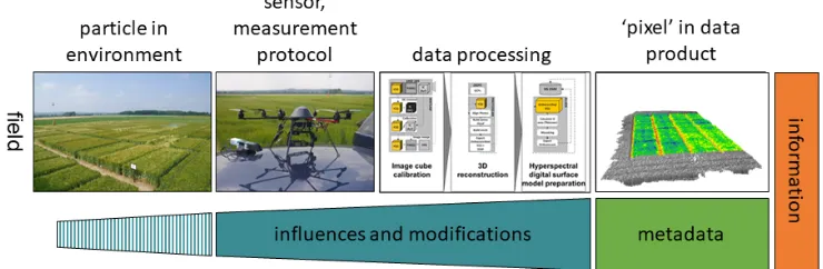
Figure 1. The path of information from a particle (e.g., pigments within the leaf), object, or surface to the data product. The spectral signal is influenced by the environment, the sensor, the measurement protocol, and data processing on the path to its representation as a pixel in a data product. In combination with metadata, this representation becomes information.
This review is structured as follows. Different technical solutions for spectral UAV sensor technology are described in Section 2. The geometric and radiometric processing steps are elaborated in Sections 3 and 4, respectively. In Section 5, we build a more complete picture of significant
Figure 1.The path of information from a particle (e.g., pigments within the leaf), object, or surface to the data product. The spectral signal is influenced by the environment, the sensor, the measurement protocol, and data processing on the path to its representation as a pixel in a data product. In combination with metadata, this representation becomes information.
Sections3and4, respectively. In Section5, we build a more complete picture of significant development steps and present the recommended best practices. The conclusions in Section6complete this review.
2. Spectral UAV Sensors
Spectral sensing can be performed using different approaches. Since in most countries the threshold to fly UAVs without permission is below a take-off weight of 30 kg, this paper will focus on sensors that can be carried by these UAVs. Generally, spectral sensors capture information in spectrally and radiometrically characterized bands. Commonly, they are distinguished by the arrangement and/or a number of bands [18,19]. Furthermore, sensors can be classified on the basis of the method by which they achieve spatial discrimination and the method by which they achieve spectral discrimination [20]. In the following subsections, we introduce several types of sensors that are available for UAVs with some example applications. Table1at the end of Section2summarizes the different sensor types.
2.1. Point Spectrometers
Point spectrometers (referred to as spectroradiometers if they are spectrally and radiometrically calibrated) capture individual spectral signatures of objects. The spectrometer’s field of view (FOV) and the distance to the object define the footprint of the measurement.
Already in 2008, point spectrometers were mounted on flying platforms (e.g., [21]). Recently, spectrometers have been miniaturized such that their size and the payload capacity of UAVs converged. In 2014, Burkart et al. [22] developed an ultra-lightweight UAV spectrometer system based on the compact Ocean Optics STS [23] for field spectroscopy. It recorded spectral information in the wavelength range of 338 nm to 824 nm, with a full width at half maximum (FWHM) of 3 nm and a FOV of 12◦, and later it was used as a flying goniometer to measure the bidirectional reflectance distribution function of vegetation [24]. Garzonio et al. [25] presented a system to measure sun-induced fluorescence in the oxygen A absorption band with the high-spectral resolution spectrometer Ocean optics USB4000 with an FWHM of 1.5 nm and a FOV of 6◦. Furthermore, UAV point spectrometers have been used to investigate the impact of environmental variables on water reflectance [26] and for intercomparison with data from a moderate resolution imaging spectroradiometer (MODIS) in Greenland [27]. Besides, UAV point measurements have been fused with multispectral 2D imaging sensors [28] and applied from fixed-wing UAVs [29], e.g., to monitor phytoplankton bloom [30]. Additionally, first attempts have been made to build low-cost whiskbroom systems for UAVs, which are able to quickly scan points on the surface [31].
The benefits of point spectrometers are their high spectral resolution, high dynamic range, high signal-to-noise ratio (SNR), and low weight. The USB4000 weighs approximately 190 g, and the STS spectrometer only weighs about 60 g. In combination with a microcontroller, the total ready-to-fly payload with the STS is only 216 g [22], allowing their installation on very small UAVs. However, since their data contains no spatial reference, auxiliary data is required for georeferencing; this makes additional devices necessary, increasing the overall weight and cost of the system (c.f. Section3.1). In addition, the data within the FOV of the spectrometer cannot be spatially resolved; i.e., each spectral measurement includes spectral information from objects within the FOV of the sensor.
2.2. Pushbroom Spectrometers
The pushbroom sensor records a line of spectral information at each exposure. By repeating the recording of individual lines during flight, a continuous spectral image over the object is obtained. Each pixel represents the spectral signature of the objects within its instantaneous FOV (IFOV) [32]. The pushbroom design has been the ‘standard’ design for large airborne imaging spectrometers for many years; however, miniaturization for small UAVs has only recently been achieved.
scanner [34] with a FWHM of 3.2 nm or 6.4 nm, depending on the slit used. In addition, pushbroom scanners have been used to detect plant diseases [35], estimate gross primary production (GPP) by means of physiological vegetation indices [36], and retrieve chlorophyll fluorescence by means of the Fraunhofer line depth method with three narrow spectral bands around the O2-A absorption feature at 760 nm [35,36]. Pushbroom sensors have also been flown together with light detection and ranging (LiDAR) systems to fuse spectral and 3D data [37]. Most of these studies were carried out with fixed-wing UAVs at flying altitudes of 330–575 m above ground level (AGL), resulting in a ground sampling distance (GSD) of 0.3–0.4 m. Pushbroom systems have also been mounted on multi-rotor UAVs, flying lower and slower, resulting in ultra-high ground sampling distances (<10 cm pixel size). Lucieer et al. [38] and Malenovsky et al. [39] achieved resolutions of up to 4 cm to map the health of Antarctic moss beds.
State-of-the-art pushbroom sensors for UAVs weigh between 0.5–4 kg (typically ~1 kg) including the lens. However, due to the large amount of data captured by such a sensor, a mini-computer with considerable storage capacity has to be flown together with the sensor, which increases the payload (Section3.2). Suomalainen et al. [40] built a hyperspectral mapping system based on off-the-shelf components. Their total system included a pushbroom spectrometer, global navigation satellite system (GNSS) receiver and inertial measurement unit (IMU), a red–green–blue (RGB) camera, and a Raspberry PI to control the system and acting as a data sink. The total weight of the system was 2 kg [40]. Recently, companies that formerly focused on full-size aircraft systems have also attempted to miniaturize their sensors for UAVs and provide self-contained systems including the sensor, GNSS/IMU, and control and storage devices (e.g., [41]).
The benefits of pushbroom devices include their high spatial and spectral resolution, and the ability to provide spatially resolved images. Compared to the point spectrometers, they are heavier and require more powerful on-board computers. Similar to point spectrometers, pushbroom systems need additional equipment on-board the UAV to enable accurate georeferencing of the data (c.f. Section3.2).
2.3. Spectral 2D Imagers
2D spectral imagers record spectral data in two spatial dimensions within every exposure. This has opened up new ways of imaging spectroscopy [42], since computer vision algorithms can be used to compose a scene from individual images, and spectral and 3D information can be retrieved from the same data and composed to (hyper)spectral digital surface models [43,44]. Since [43] first attempted to categorize 2D imagers (then commonly referred to as image-frame cameras or central perspective images [32]), new technologies have appeared. Today, 2D imagers exist that record the spectral bands sequentially or altogether within a snapshot. In addition, multi-camera systems record spectral bands synchronously with several cameras. In the following sections, these different technologies are reviewed.
2.3.1. Multi-Camera 2D Imagers
suited for taking images during UAV movement. Newer Tetracam cameras now also use global shutter in the Macaw model.
Recently, similar but more compact systems have appeared on the market. Among them are the MicaSense Parrot Sequoia and RedEdge(-m) [51,52] with four and five spectral bands (blue, green, red, red edge, near-infrared), and the MAIA camera [53], with nine bands captured by separate imaging sensors that operate simultaneously. Such cameras were used to assess forest health [54], leaf area index in mangrove forests [55] and grapevine disease infestation [56]. In addition, self-built multi-camera spectral 2D systems have been used to identify water stress [57] as well as crop biomass and nitrogen content [58].
2.3.2. Sequential 2D Imagers
Sequential band systems record bands or sets of bands sequentially in time, with a time lag between two consecutive spectral bands. These systems have often been called image-frame sensors [43,44,59,60]. An example of such a system is the Rikola hyperspectral imager by Senop Oy [61] that is based on the tunable Fabry–Pérot Interferometer (FPI). The camera weighs 720 g. The desired spectral bands are obtained by scanning the spectral range with different air gap values within the FPI [44,62]. The current commercial camera has approximately 1010×1010 pixels, providing a vertical and horizontal FOV of 36.5◦[61,63]. In total, 380 spectral bands can be selected with a 1-nm spectral step in the spectral range of approximately 500–900 nm, but in typical UAV operation, 50–100 bands are collected. The FWHM increases with the wavelength if the order of interference and the reflectance of the mirrors remain the same [64]. However, in practical implementation of the Rikola camera, the resulting FWHMs are similar in the visible and near-infrared (NIR) ranges: approximately 5–12 nm. The Rikola HSI records up to 32 individual bands within a second; so, for example, a hypercube with 60 freely selectable individual bands can be captured within a 2-s interval. Recently, a sort-wave infrared (SWIR) range prototype camera was developed, with a spectral range of 0.9–1.7µm and an image size of 320×256 pixels [65,66].
Benefits of the sequential 2D imagers are the comparably high spatial resolution and the flexibility to choose spectral bands. At the same time, the more bands that are chosen, the longer it takes to record all of them. In mobile applications, the bands in individual cubes have spatial offsets that need to be corrected in post-processing (c.f. Section3.3.2) [44,67,68]. The frame rate, exposure time, number of bands, and flying height limit the flight speed in tunable filter-based systems. The FPI cameras have been used in various environmental remote sensing studies, including precision agriculture [44,69–71], peat production area moisture monitoring [65], tree species classification, forest stand parameter estimation, biodiversity assessment [72–74], mineral exploration [68], and detection of insect damage in forests [60,75].
2.3.3. Snapshot 2D Imagers
Snapshot systems record all of the bands at the same time [43,76,77], which has the advantage that no spatial co-registration needs to be carried out [43]. Currently, multi-point and filter-on-chip snapshot systems exist for UAVs.
Multi-point spectrometer
The advantage of multi-point 2D imagers is that they record all of the spectral information for each point in the image at the same time, and typical integration times are very short due to the high light throughput. However, the disadvantage is the relatively low spatial resolution of the spectral information.
Mosaic filter-on-chip cameras
In the mosaic filter-on-chip technology, each pixel carries a spectral filter that has a certain transmission, such as the principle of a Bayer pattern in an RGB camera. The combined information of the pixels within a mosaic or tiles then represents the spectral information of the area seen by the tile. The technology is based on a thin wafer on top of a monochromatic complementary metal–oxide semiconductor (CMOS) sensor in which the wafer contains band pass filters that isolate spectral wavelengths according to the Fabry–Pérot interference principle [81,82]. The wafers are produced in a range of spatial configurations, including linear, mosaic, and tile-based filters. This technique was developed by Imec using the FPI filters to provide different spectral bands [81]. Currently, the chip is available for the range of 470–630 nm in 16 (4×4 pattern) bands with a spatial resolution of 512×256 pixels, and in the range of 600–1000 nm in 25 bands (5×5 pattern) with a spatial resolution of 409×216 pixels. The FWHM is below 15 nm for both systems. The two chips are integrated into cameras by several companies, and weigh below 400 g (e.g., [83,84]). So far, only first attempts with this new technology have been published [85,86], including a study on how to optimize the demosaicing of the images [87]. Recently, Imec has announced a SWIR version of the camera [88].
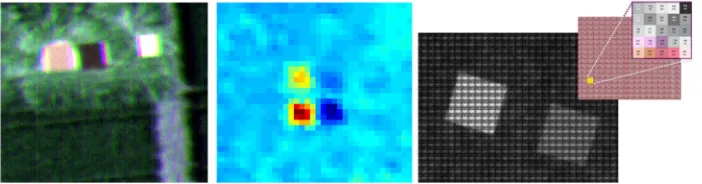
The advantage of filter-on-chip cameras is that they record all of the bands at the same time. Additionally, they are very light, and can be carried by small UAVs. The disadvantage is that each band is just measured once within each tile and thus, accurate spectral information for one band is only available once every few pixels. Currently, this is tackled by slightly defocusing the camera and interpolation techniques. They have a higher spatial resolution than multi-point spectrometers, but the radiometric performance of the filter-on-chip technology has not yet reached the quality of established sensing principles that is used in point and line scanning devices. This mainly results from the technical challenges during the manufacturing process (i.e., strong variation of the thickness of the filter elements between adjacent pixels) and the novelty of the technique. Figure2shows images captured by a sequential 2D imager, a multi-point spectrometer, and a filter-on-chip snapshot camera.
Remote Sens. 2018, 10, x FOR PEER REVIEW 6 of 42
Mosaic filter-on-chip cameras
In the mosaic filter-on-chip technology, each pixel carries a spectral filter that has a certain transmission, such as the principle of a Bayer pattern in an RGB camera. The combined information of the pixels within a mosaic or tiles then represents the spectral information of the area seen by the tile. The technology is based on a thin wafer on top of a monochromatic complementary metal–oxide semiconductor (CMOS) sensor in which the wafer contains band pass filters that isolate spectral wavelengths according to the Fabry–Pérot interference principle [81,82]. The wafers are produced in a range of spatial configurations, including linear, mosaic, and tile-based filters. This technique was developed by Imec using the FPI filters to provide different spectral bands [81]. Currently, the chip is available for the range of 470–630 nm in 16 (4 × 4 pattern) bands with a spatial resolution of 512 × 256 pixels, and in the range of 600–1000 nm in 25 bands (5 × 5 pattern) with a spatial resolution of 409 × 216 pixels. The FWHM is below 15 nm for both systems. The two chips are integrated into cameras by several companies, and weigh below 400 g (e.g., [83,84]). So far, only first attempts with this new technology have been published [85,86], including a study on how to optimize the demosaicing of the images [87]. Recently, Imec has announced a SWIR version of the camera [88].
[image:6.595.125.476.513.605.2]The advantage of filter-on-chip cameras is that they record all of the bands at the same time. Additionally, they are very light, and can be carried by small UAVs. The disadvantage is that each band is just measured once within each tile and thus, accurate spectral information for one band is only available once every few pixels. Currently, this is tackled by slightly defocusing the camera and interpolation techniques. They have a higher spatial resolution than multi-point spectrometers, but the radiometric performance of the filter-on-chip technology has not yet reached the quality of established sensing principles that is used in point and line scanning devices. This mainly results from the technical challenges during the manufacturing process (i.e., strong variation of the thickness of the filter elements between adjacent pixels) and the novelty of the technique. Figure 2 shows images captured by a sequential 2D imager, a multi-point spectrometer, and a filter-on-chip snapshot camera.
Figure 2. Example images captured by the sequential Rikola Fabry–Pérot Interferometer (FPI) (left), multi-point spectrometer CUBERT Firefleye (center) and filter-on-chip Imec NIR (right) 2D imagers. The excerpt shows one 5 × 5 tile used to capture the spectral information.
Spatiospectral filter-on-chip cameras
To address the latter, a modified version of the filter-on-chip camera called COSI Cam has been developed [89]. This sensor no longer uses a small number of spectral filters in a tiled or pixel-wise mosaic arrangement. Instead, a larger number of narrow band filters are used, which are sampled densely enough to have continuous spectral sampling. The filters are arranged in a line-wise fashion, with a n amount of lines (a small number, five or eight) of the same filter next to each other, followed by n lines of spectrally adjacent filter bands. In this arrangement, filters on adjacent pixels only vary slightly in thickness, leading to much cleaner spectral responses than the 4 × 4 and 5 × 5 pattern. The COSI Cam prototype [89] was the first camera using such a chip, capturing more than 100 spectral bands in the range of 600 nm–900 nm. In a further development, by using two types of filter material on the chip, a larger spectral range of 475 nm–925 nm was achieved (ButterflEYE LS; [90]) with a spectral sampling of less than 2.5 nm.
Figure 2.Example images captured by the sequential Rikola Fabry–Pérot Interferometer (FPI) (left), multi-point spectrometer CUBERT Firefleye (center) and filter-on-chip Imec NIR (right) 2D imagers. The excerpt shows one 5×5 tile used to capture the spectral information.
Spatiospectral filter-on-chip cameras
slightly in thickness, leading to much cleaner spectral responses than the 4×4 and 5×5 pattern. The COSI Cam prototype [89] was the first camera using such a chip, capturing more than 100 spectral bands in the range of 600 nm–900 nm. In a further development, by using two types of filter material on the chip, a larger spectral range of 475 nm–925 nm was achieved (ButterflEYE LS; [90]) with a spectral sampling of less than 2.5 nm.
Physically, these cameras are filter-on-chip cameras, but their filter arrangement requires a different mode of operation. Their operation includes scanning over an area, and is similar to the operation of a pushbroom camera. Therefore, these sensors are also referred to as spatiospectral scanners. The 2D sensor can be seen as a large array of 1D sensors, each capturing a different spectral band (in fact,nduplicate lines per band). To capture all of the spectral bands at every location, a new image has to be captured every time the platform has moved the equivalent ofnlines. This is achieved by limiting the flying speed and operating the camera with a high frame rate (typically 30 frames per second (fps)), which means a larger portion of the flying time is used for collecting information. A specialized processing workflow then generates the full image cube for the scene [90].
Due to their improved design, the radiometric quality of the spectrospatial cameras is better compared to the classical filter-on-chip design. At the same time, their data enables the reconstruction of the 3D geometry similar to other 2D imagers due to the 2D spatial information within the images. Sima et al. [91] showed that a good spatial co-registration can be achieved that also allows extraction of digital surface models (DSMs). The drawback of these systems is that they require large storage capacity and a lower flying speed to obtain full coverage over the target of interest. A further challenge in this kind of sensor is that each band has different anisotropy effects as a result of having different view angles to the object.
Characterized (modified) RGB cameras
RGB and modified RGB cameras (e.g., where the infrared filter is removed, and so called color-infrared cameras (CIR) with green, red and near-infrared bands) can also be used to capture spectral data if they are spectrally and radiometrically characterized, and the automatic image adjustment is turned off. These cameras only have a very limited number of rather wide spectral bands, but have a very high spatial resolution at comparatively low cost. An example is the Canon s110 NIR, which records green (560 nm, FWHM: 50 nm), red (625 nm, FWHM: 90 nm), and near-infrared (850 nm, FWHM: 100 nm) bands at 3000 by 4000 pixels. For some cameras, firmware enhancements such as the Canon Hack Development Kit (CHDK Community, 2017) are available and provide additional functionality beyond the native camera firmware, which is potentially useful for remote sensing activities. Berra et al. [92] demonstrated how to characterize such cameras and compared the results of multi-temporal flights to map phenology to Landsat 8 data.
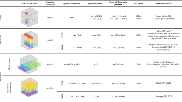
Table 1.Different spectral sensor types for unmanned aerial vehicle (UAV) sensing systems with properties of example sensors. The exact numbers may vary between different models, and should just be taken as indication. The visualizations indicate the image cube slices recorded during each measurement of a sensor type (adapted from drawings provided by Stefan Livens). The information in the table is composed of information found in the literature, on websites of the manufacturers, and personal correspondence with Stefan Livens from VITO (for the COSI cam), Trond Løke from HySpex (for the Mjolnir), and Robert Parker from Micasense (for the RedEdge-m). FWHM: full width at half maximum.
Data Cube Slice Scanning
Dimension Spatial Resolution Spectral Bands **
Spectral Resolution
(FWHM) Bit Depth Example Sensors
Point
Remote Sens. 2018, 10, x FOR PEER REVIEW 8 of 49 Table 1. Different spectral sensor types for unmanned aerial vehicle (UAV) sensing systems with properties of example sensors. The exact numbers may vary between different models, and should just be taken as indication. The visualizations indicate the image cube slices recorded during each measurement of a sensor type (adapted from drawings provided by Stefan Livens). The information in the table is composed of information found in the literature, on websites of the manufacturers, and personal correspondence with Stefan Livens from VITO (for the COSI cam), Trond Løke from HySpex (for the Mjolnir), and Robert Parker from Micasense (for the RedEdge-m). FWHM: full width at half maximum.
Data Cube Slice Scanning
Dimension Spatial Resolution Spectral Bands **
Spectral Resolution
(FWHM) Bit Depth Example Sensors
Po
int spatial none ++++ (1024)
+++++ (3648)
++++ (1–12 nm) +++++ (0.1–10 nm)
12 bit 16 bit
Ocean Optics STS Ocean Optics USB4000
P
u
sh
broom spatial
VNIR +++ (1240) ++++ (200) +++ (3.2–6.4 nm) 12 bit
HySpex Mjolnir V Specim AisaKESTREL 10, Headwall
micro-hyperspec/nano-hyperspec, Bayspec OCI, Resonon Pika
SWIR +++ (620) ++++ (300) +++ (~6 nm) 16 bit
HySpex Mjolnir S (970–2500 nm) Specim AisaKESTREL 16
(600–1640 nm)
2D im
ager Mult
i-ca
m
era
spatial +++ (1280 × 960) + (5) + (10–40 nm) 12 bit
Micasense RedEdge-m Parrot Sequoia, Tetracam Mini MCA,
macaw Sequ en ti al (m ulti-) b and spectral
VNIR +++ (1000 × 1000) +++ (100) +++ (5–12 nm) 12 bit Rikola FPI VNIR
spatial none ++++(1024)
+++++(3648)
++++(1–12 nm)
+++++(0.1–10 nm)
12 bit 16 bit
Ocean Optics STS Ocean Optics USB4000
Pushbr
oom
Remote Sens. 2018, 10, x FOR PEER REVIEW 8 of 49 Table 1. Different spectral sensor types for unmanned aerial vehicle (UAV) sensing systems with properties of example sensors. The exact numbers may vary between different models, and should just be taken as indication. The visualizations indicate the image cube slices recorded during each measurement of a sensor type (adapted from drawings provided by Stefan Livens). The information in the table is composed of information found in the literature, on websites of the manufacturers, and personal correspondence with Stefan Livens from VITO (for the COSI cam), Trond Løke from HySpex (for the Mjolnir), and Robert Parker from Micasense (for the RedEdge-m). FWHM: full width at half maximum.
Data Cube Slice Scanning
Dimension Spatial Resolution Spectral Bands **
Spectral Resolution
(FWHM) Bit Depth Example Sensors
Po
int spatial none ++++ (1024)
+++++ (3648)
++++ (1–12 nm) +++++ (0.1–10 nm)
12 bit 16 bit
Ocean Optics STS Ocean Optics USB4000
P
u
sh
broom spatial
VNIR +++ (1240) ++++ (200) +++ (3.2–6.4 nm) 12 bit
HySpex Mjolnir V Specim AisaKESTREL 10, Headwall
micro-hyperspec/nano-hyperspec, Bayspec OCI, Resonon Pika
SWIR +++ (620) ++++ (300) +++ (~6 nm) 16 bit
HySpex Mjolnir S (970–2500 nm) Specim AisaKESTREL 16
(600–1640 nm)
2D im
ager Mult
i-ca
m
era
spatial +++ (1280 × 960) + (5) + (10–40 nm) 12 bit
Micasense RedEdge-m Parrot Sequoia, Tetracam Mini MCA,
macaw Sequ en ti al (m ulti-) b and spectral
VNIR +++ (1000 × 1000) +++ (100) +++ (5–12 nm) 12 bit Rikola FPI VNIR spatial
VNIR +++(1240) ++++(200) +++(3.2–6.4 nm) 12 bit
HySpex Mjolnir V Specim AisaKESTREL 10, Headwall
micro-hyperspec/nano-hyperspec, Bayspec OCI, Resonon Pika
SWIR +++(620) ++++(300) +++(~6 nm) 16 bit
HySpex Mjolnir S (970–2500 nm) Specim AisaKESTREL 16
(600–1640 nm)
2D
imager
Multi-camera
Remote Sens. 2018, 10, x FOR PEER REVIEW 8 of 49 Table 1. Different spectral sensor types for unmanned aerial vehicle (UAV) sensing systems with properties of example sensors. The exact numbers may vary between different models, and should just be taken as indication. The visualizations indicate the image cube slices recorded during each measurement of a sensor type (adapted from drawings provided by Stefan Livens). The information in the table is composed of information found in the literature, on websites of the manufacturers, and personal correspondence with Stefan Livens from VITO (for the COSI cam), Trond Løke from HySpex (for the Mjolnir), and Robert Parker from Micasense (for the RedEdge-m). FWHM: full width at half maximum.
Data Cube Slice Scanning
Dimension Spatial Resolution Spectral Bands **
Spectral Resolution
(FWHM) Bit Depth Example Sensors
Po
int spatial none ++++ (1024)
+++++ (3648)
++++ (1–12 nm) +++++ (0.1–10 nm)
12 bit 16 bit
Ocean Optics STS Ocean Optics USB4000
P
u
sh
broom spatial
VNIR +++ (1240) ++++ (200) +++ (3.2–6.4 nm) 12 bit
HySpex Mjolnir V Specim AisaKESTREL 10, Headwall
micro-hyperspec/nano-hyperspec, Bayspec OCI, Resonon Pika
SWIR +++ (620) ++++ (300) +++ (~6 nm) 16 bit
HySpex Mjolnir S (970–2500 nm) Specim AisaKESTREL 16
(600–1640 nm)
2D im
ager Mult
i-ca
m
era
spatial +++ (1280 × 960) + (5) + (10–40 nm) 12 bit
Micasense RedEdge-m Parrot Sequoia, Tetracam Mini MCA,
macaw Sequ en ti al (m ulti-) b and spectral
VNIR +++ (1000 × 1000) +++ (100) +++ (5–12 nm) 12 bit Rikola FPI VNIR
spatial +++(1280×960) +(5) +(10–40 nm) 12 bit
Micasense RedEdge-m Parrot Sequoia, Tetracam Mini MCA,
macaw
Sequential
(multi-)
band
Remote Sens. 2018, 10, x FOR PEER REVIEW 9 of 49
SWIR ++ (320 × 256) ++ (30) ++ (20–30 nm) Prototype FPI SWIR
sna p sh o t Mult
i-point none + (50 × 50) +++ (125) +++ (5–25 nm) 12 bit Cubert FireFleye
Filt
er-on
-ch
ip
none
VIS ++ (512 × 272) ++ (16) ++ (5–10 nm) 10 bit imec SNm4x4 *
NIR ++ (409 × 216) ++ (25) ++ (5–10 nm) 10 bit imec SNm5x5 *
C h aract erized (m od if ied)
RGB none ++++ 3000 × 4000 + (3) + (50–100 nm) 12 bit canon s110 (NIR) spectral
VNIR +++(1000×1000) +++(100) +++(5–12 nm) 12 bit Rikola FPI VNIR
Remote Sens.2018,10, 1091 9 of 42
Table 1.Cont.
Data Cube Slice Scanning
Dimension Spatial Resolution Spectral Bands **
Spectral Resolution
(FWHM) Bit Depth Example Sensors
2D
imager
snapshot
Multi-point
SWIR ++ (320 × 256) ++ (30) ++ (20–30 nm) Prototype FPI SWIR
sna p sh o t Mult
i-point none + (50 × 50) +++ (125) +++ (5–25 nm) 12 bit Cubert FireFleye
Filt
er-on
-ch
ip
none
VIS ++ (512 × 272) ++ (16) ++ (5–10 nm) 10 bit imec SNm4x4 *
NIR ++ (409 × 216) ++ (25) ++ (5–10 nm) 10 bit imec SNm5x5 *
C h aract erized (m od if ied)
RGB none ++++ 3000 × 4000 + (3) + (50–100 nm) 12 bit canon s110 (NIR)
none +(50×50) +++(125) +++(5–25 nm) 12 bit Cubert FireFleye
Filter
-on-chip
SWIR ++ (320 × 256) ++ (30) ++ (20–30 nm) Prototype FPI SWIR
sna p sh o t Mult
i-point none + (50 × 50) +++ (125) +++ (5–25 nm) 12 bit Cubert FireFleye
Filt
er-on
-ch
ip
none
VIS ++ (512 × 272) ++ (16) ++ (5–10 nm) 10 bit imec SNm4x4 *
NIR ++ (409 × 216) ++ (25) ++ (5–10 nm) 10 bit imec SNm5x5 *
C h aract erized (m od if ied)
RGB none ++++ 3000 × 4000 + (3) + (50–100 nm) 12 bit canon s110 (NIR) none
VIS ++(512×272) ++(16) ++(5–10 nm) 10 bit imec SNm4x4 *
NIR ++(409×216) ++(25) ++(5–10 nm) 10 bit imec SNm5x5 *
Characterized (modified)
RGB
SWIR ++ (320 × 256) ++ (30) ++ (20–30 nm) Prototype FPI SWIR
sna p sh o t Mult
i-point none + (50 × 50) +++ (125) +++ (5–25 nm) 12 bit Cubert FireFleye
Filt
er-on
-ch
ip
none
VIS ++ (512 × 272) ++ (16) ++ (5–10 nm) 10 bit imec SNm4x4 *
NIR ++ (409 × 216) ++ (25) ++ (5–10 nm) 10 bit imec SNm5x5 *
C h aract erized (m od if ied)
RGB none none ++++ 3000 × 4000 ++++3000×4000 + (3) +(3)+ (50–100 nm) +(50–100 nm)12 bit canon s110 (NIR) 12 bit canon s110 (NIR)
Spatiospectral
Remote Sens. 2018, 10, x FOR PEER REVIEW 10 of 49
Spat
ios
p
ect
ral
spatiospectral ++++ 2000 ++ (160) ++ (5–10 nm) 8 bit COSI cam Cubert ButterflEYE LS
* Sold by different companies, e.g., Cubert Butterfly VIS/NIR, ximea MQ022HG-IM-SM4X4-VIS/MQ022HG-IM-SM5X5-NIR, photonFocus MV1-D2048x1088-HS03-96-G2/MV1-D2048x1088-HS02-96-G2. ** number of spectral bands depends on the configuration and binning of the devices and should just be used as a reference.
spatiospectral ++++2000 ++(160) ++(5–10 nm) 8 bit COSI cam
Cubert ButterflEYE LS
3. Integration of Sensors and Geometric Processing
Accurate geometric processing is a crucial task in the data processing workflow for UAV datasets. Fundamental steps include the determination of the sensor interior characteristics of the sensor system (interior orientation), the exterior orientation of the data sequence (position and rotation of the sensor during the data capture), and the object geometric model to find the geometric relationship between the object and the recorded radiance value.
Accurate position and orientation information is required to compute the location of each pixel on the ground. Full-size airborne hyperspectral sensors follow the pushbroom design, and some can use a survey-grade differential GNSS receiver (typically multi-constellation and dual frequency capabilities) and IMU to determine the position and orientation (pitch, roll, and heading) of the image lines. When post-processed against a GNSS base station established over a survey mark at a short baseline (within 5–10 km), a positioning accuracy of 1–4 cm can be achieved for the on-board GNSS antenna, after which propagation of all of the pose-related errors typically results in 5–10 cm direct georeferencing accuracy of UAS image data. This can be further improved by using ground control points (GCPs) measured with a differential GNSS rover on the ground or a total station survey [94–97]. One of the challenges in hyperspectral data collection from UAVs is the limitation in weight and size of the total sensor payload. Survey-grade GNSS and IMU sensors tend to be relatively heavy, bulky, and expensive, e.g., fiber optic gyro (FOG) IMUs providing absolute accuracy in orientation of <0.05◦[98]. Development in microelectromechanical systems (MEMS) has resulted in small and lightweight IMUs suitable for UAV applications; however, traditionally, the absolute accuracy of these MEMS IMUs has been relatively poor (e.g., typically ~1◦absolute accuracy in pitch, roll, and yaw) [98]. The impact of a 1◦ error at a flying height of 50 m above ground level (AGL) is a 0.87-m geometric offset for a pixel on the ground. If we consider the key benefit of UAV remote sensing to be the ability to collect sub-decimeter resolution imagery, then such a large error is potentially unacceptable. The combined error in pitch, roll, heading, and position can make this even worse. There is an important requirement for the optimal combination of sensors to determine accurate position and orientation (pose) of the spectral sensor during acquisition (which also requires accurate time synchronization), or an appropriate geometric processing strategy based on image matching and ground control points (GCPs).
3.1. Georeferencing of Point Spectrometer Data
weighted within their FOV, and the configuration of the fiber and fore optic might influence the measured signal [101].
3.2. Georeferencing of Pushbroom Scanner Data
Pushbroom sensors need to move to build up a spatial image of a scene. Typically, these sensors collect 20–100 frames per second (depending on integration time and camera specifications). The slit width, lens focal length, and integration time determine the spatial resolution of the pixels in the along-track direction (i.e., flight direction). The number of pixels on the sensor array (i.e., number of columns) and the focal length of the sensor determine the spatial resolution of the pixels in the across-track direction. To accurately map the spatial location of each pixel in the scene, several parameters need to be provided or determined: camera/lens distortion parameters, sensor location (XYZ), sensor absolute orientation (pitch, roll, and heading), and surface model of the terrain. Pushbroom sensors are particularly sensitive to flight dynamics in pitch, roll, and heading, which makes it challenging to perform a robust geometric correction or orthorectification. For dynamic UAV airframes, such as multi-rotors, this is particularly challenging.
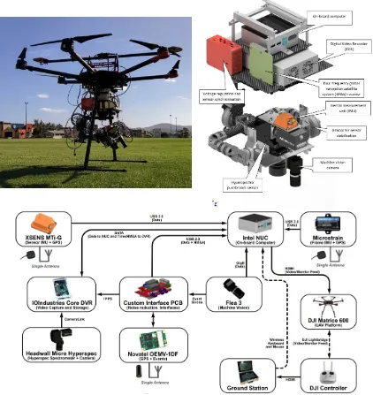
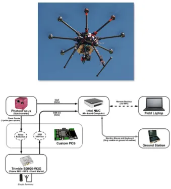
Lucieer et al. [38] and Malenovský et al. [39] developed and used an early hyperspectral multi-rotor prototype in Antarctica that did not use GNSS/IMU observations, but rather relied on a dense network of GCPs for geometric rectification based on triangulation/rubber-sheeting. This prototype was later upgraded to include synchronized GNSS/IMU data (Figure3) in order to enable orthorectification using the PARGE geometric rectification software [102,103].
With the use of a limited number of GCPs and/or on-board GNSS coordinates, machine vision imagery can be used to determine the position and orientation of a hyperspectral sensor without the need for complex and expensive GNSS/IMU sensors. The main advantage of machine vision imagery is that it can be used in rigorous photogrammetric modeling [104], SfM [105], or simultaneous localization and mapping (SLAM) [106] workflows to extract 3D terrain information and pose information simultaneously. Suomalainen et al. [40] developed a hyperspectral pushbroom system with a synchronized GNSS/IMU unit for orthorectification; they used a photogrammetric approach based on SfM to improve the accuracy of the on-board navigation-grade GNSS receiver and derive a digital surface model for orthorectification. Habib et al. [107] and Ramirez-Paredes et al. [108] presented approaches for the georectification of hyperspectral pushbroom imagery that were purely based on imagery and image matching. Their approaches are attractive, as a fully image-based approach reduces the complexity of sensor integration on board the UAV. However, in order to achieve a high absolute accuracy, accurate GCP measurements still need to be obtained, or an accurate on-board GNSS needs to be employed. In addition, to match the frame rate of a hyperspectral sensor, a lot of machine vision data will have to be stored and processed (potentially thousands of images per flight).
Remote Sens. 2018, 10, x FOR PEER REVIEW 13 of 42
Figure 3. TerraLuma pushbroom system: Image (top left) and drawing of the sensor payload (top right) and device interaction flow chart (bottom; CAD design and flow chart: Richard Ballard, TerraLuma group).
3.3. Georeferencing of 2D Imager Data
3.3.1. Snapshot 2D Imagers
The major advantage of snapshot 2D imagers is that the spatial patterns in each image frame can be used in an SfM workflow. Through the selection of an optimal spectral band or the use of the raw 2D hyperspectral mosaic, the SfM process allows for the extraction and matching of image features. The resulting bundle adjustment will then calculate the position and orientation for each image frame without the need for GNSS/IMU sensors (although the image-matching phase can be assisted with GNSS/IMU observations), which reduces the complexity of the setup (Figure 4). Since this approach derives the relative position and orientation of the images, a scene with relative scaling can be generated. For several applications, this is already sufficient, and the approach is appealing, since one can forgo the additional weight and complexity of a GNSS/INS approach. Still, with the aid of an accurate on-board GNSS receiver or GCPs, geometrically accurate orthomosaics can be created (with a typical absolute accuracy of 1–2 pixels). One of the issues with this approach is that 2D imagers
Figure 3. TerraLuma pushbroom system: Image (top left) and drawing of the sensor payload (top right) and device interaction flow chart (bottom; CAD design and flow chart: Richard Ballard, TerraLuma group).
3.3. Georeferencing of 2D Imager Data
3.3.1. Snapshot 2D Imagers
of an accurate on-board GNSS receiver or GCPs, geometrically accurate orthomosaics can be created (with a typical absolute accuracy of 1–2 pixels). One of the issues with this approach is that 2D imagers tend to have a lower spatial resolution, which can affect the number of matching features found in the SfM process. This can result in poor performance in image matching in complex terrain/vegetation, which has a direct impact on the quality of the spectral orthomosaic. This can be compensated by merging the low-resolution hyperspectral information with, e.g., a higher resolution panchromatic image [43]. An additional benefit of 2D imagers is that an initial bundle adjustment can be followed by an optional dense matching approach, which then allows the generation of high-resolution 3D hyperspectral point clouds and surface models (c.f. Section5.4).
Remote Sens. 2018, 10, x FOR PEER REVIEW 14 of 42
[image:13.595.129.468.220.594.2]tend to have a lower spatial resolution, which can affect the number of matching features found in the SfM process. This can result in poor performance in image matching in complex terrain/vegetation, which has a direct impact on the quality of the spectral orthomosaic. This can be compensated by merging the low-resolution hyperspectral information with, e.g., a higher resolution panchromatic image [43]. An additional benefit of 2D imagers is that an initial bundle adjustment can be followed by an optional dense matching approach, which then allows the generation of high-resolution 3D hyperspectral point clouds and surface models (c.f. Section 5.4).
Figure 4. TerraLuma 2D imager system (top) with exemplary device interaction flow chart (bottom; source: Richard Ballard, TerraLuma group).
3.3.2. Georeferencing of Sequential and Multi-Camera 2D Imagers
The multispectral and hyperspectral sensors based on multiple cameras or tunable filters produce non-aligned spectral bands. The straightforward approach would be to determine the exterior orientations of each band individually using SfM. If the number of bands is large, for example 20 or 100, the separate orientation of each band can result in a significant computational challenge, and therefore, solutions based on image registration are more feasible [109]. The transformation can be two-dimensional (such as rigid body, Helmert, affine, polynomial, or projective) or three-dimensional, based on the collinearity model and accounting for the object’s 3D structure, i.e., the orthorectification [110].
Jhan et al. [111] presented an approach utilizing the relative calibration information and projective transformations for the Mini-MCA lightweight camera, which is composed of six individual, rigidly assembled cameras. They used a laboratory calibration process to determine the relative orientations of individual cameras with respect to the master camera in the multi-camera system; the relative orientations of the master camera (red band) and an additional RGB camera were determined.
Figure 4.TerraLuma 2D imager system (top) with exemplary device interaction flow chart (bottom; source: Richard Ballard, TerraLuma group).
3.3.2. Georeferencing of Sequential and Multi-Camera 2D Imagers
Jhan et al. [111] presented an approach utilizing the relative calibration information and projective transformations for the Mini-MCA lightweight camera, which is composed of six individual, rigidly assembled cameras. They used a laboratory calibration process to determine the relative orientations of individual cameras with respect to the master camera in the multi-camera system; the relative orientations of the master camera (red band) and an additional RGB camera were determined. The RGB camera was oriented with bundle-block adjustment, and the exterior orientations of the rest of the bands were calculated based on the relative orientations and the exterior orientations of the reference camera. An accuracy of 0.33 pixels was reported in the registered images. Several researchers reported accuracies on the level of approximately two pixels when using approaches based on 2D transformations with the mini-MCA camera [112–114].
In the cases of tunable filters such as the Rikola camera, each band has a unique exterior orientation. Honkavaara et al. [67] showed that the geometric challenges increase with the decreasing flight height and increasing flight speed, time difference between the bands, and height differences among the objects. In several studies, good results have been reported when using 2D image transformations in flat environments [44,115]. If the object has great height differences, such as forest, rugged terrain, and built areas, the 2D image transformations do not give accurate solutions in general cases; however, good results were reported also in a rugged environment when using 2D image transformations if combined with image capture based on stopping while taking each hypercube [68]. Image registration based on physical exterior orientation parameters and orthorectification should be used when operating these tunable filter sensors from mobile platforms in environments where the object of interest has significant height differences. Honkavaara et al. [67] developed a rigorous and efficient approach to calculate co-registered orthophoto mosaics of tunable filter images. The process include the determination of orientations of three to five reference bands using SfM, subsequent matching of the unoriented bands to the reference bands, calculation of their exterior orientations, and the orthorectification of all of the bands. Registration errors of less than a pixel were obtained in forested environments. The authors emphasized the need for proper block design in order to achieve the desired precision.
4. Radiometric Processing Workflow
4.1. General Procedure for Generating Reflectance Maps from UAVs
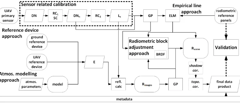
Radiometric processing transforms the readings of a sensor into useful data. First, sensor-related radiometric and spectral calibration needs to be carried out. Second, transformation to top-of-canopy reflectance based on radiometric reference panels and/or an empirical line method (ELM), secondary reference devices, or atmospheric modeling needs to be carried out. Third, influences of the object reflectance anisotropy (bidirectional reflectance distribution function, BRDF) effects, and shadows can be normalized. Schott [116] calls this entire multi-step process the image chain approach. The different calibration schemes are outlined in Figure5. These steps can be carried out sequentially as independent steps, which has been the typical approach in the classical approaches used for the airborne and spaceborne applications, for example, as implemented in the ATmospheric CORrection (ATCOR) [102]. UAVs also provide some novel aspects to be considered.
(e.g., from multiple images) are averaged, as is often done during orthomosaic generation from 2D images [42]. In every case, the data needs to be calibrated. In the following subsections, the sensor calibration (Section4.2) and the image data calibration (Section4.3) processes are described in detail.
[image:15.595.90.507.143.325.2]Remote Sens. 2018, 10, x FOR PEER REVIEW 16 of 42
Figure 5. The full data processing workflow to create a reflectance data product. First, sensor-related calibration procedures are carried out. Relative calibration (RC1) and spectral calibration (SC) transform the digital numbers (DN) of the sensor to normalized DN (DNn). Further, absolute radiometric calibration (RC2) can be carried out to generate at-sensor radiance (Ls). Second, the data is transformed to reflectance factors (R) with the empirical line method (ELM), based on a second radiometrically calibrated reference device on the ground, the UAV, or models. Geometric processing (GP) is an estimation of the relative position and orientation of the measurements, and composes the data into a scene. Radiometric block adjustment can be used at different steps in the process to optimize the radiometry of the scene and correct for bidirectional reflectance distribution function (BRDF) effects. The geometric processing (GP) composes the data into a scene. Additional modules may then transform the reflectance factors in the scene to reflectance quantities (c.f. Section 4.4), and shadows and topography effects may be corrected. Independent radiometric reference targets are used to validate the data. The processing procedures are tracked in metadata to allow an accurate interpretation of the results.
4.2. Sensor-Related Calibration
Radiometric sensor calibration determines the radiometric response of an individual sensor [120–122]. The calibration process includes several phases: a relative radiometric calibration, which aims for a uniform output across the pixels and time, a spectral calibration, which determines the spectral response of the bands, and an absolute radiometric calibration, which determines the transformation from pixel values to the physical unit radiance. A comprehensive review on calibration procedures for high-resolution radiance measurements can be found in Jablonski et al., [123] and Yoon and Kacker [124]. In the following, we will focus on sensor calibration procedures that are required to generate reflectance maps from spectral UAV data. These procedures will provide sensor-specific calibration factors that are applied to the captured spectrometric datasets. While the calibration steps are essentially the same for point, line, and 2D imagers, the complexity increases with data dimension, since every pixel needs to be characterized and calibrated. In many cases, researchers have implemented their own calibration procedures for small spectrometers or spectral imagers used in UAVs, since either the systems have been experimental setups, or the sensor manufacturers of small-format sensors have not provided calibration files or suitable calibration procedures. The examples in this section are taken from studies with the point spectrometer Ocean Optics STS-VIS [22] and USB 4000 [25], the pushbroom system Headwall Photonics Micro-Hyperspec [38,125], other custom-made pushbroom sensors [40,126], 2D imagers Cubert Firefleye [43,127–129], Rikola FPI [68], and Tetracam MCA and mini-MCA models [50,130,131].
4.2.1. Relative Radiometric Calibration
Relative radiometric calibration transforms the output of the sensor to normalized DNs (DNn), which have a uniform response over the entire image during the time of operation [121]. This
Figure 5.The full data processing workflow to create a reflectance data product. First, sensor-related calibration procedures are carried out. Relative calibration (RC1) and spectral calibration (SC) transform
the digital numbers (DN) of the sensor to normalized DN (DNn). Further, absolute radiometric
calibration (RC2) can be carried out to generate at-sensor radiance (Ls). Second, the data is transformed
to reflectance factors (R) with the empirical line method (ELM), based on a second radiometrically calibrated reference device on the ground, the UAV, or models. Geometric processing (GP) is an estimation of the relative position and orientation of the measurements, and composes the data into a scene. Radiometric block adjustment can be used at different steps in the process to optimize the radiometry of the scene and correct for bidirectional reflectance distribution function (BRDF) effects. The geometric processing (GP) composes the data into a scene. Additional modules may then transform the reflectance factors in the scene to reflectance quantities (c.f. Section4.4), and shadows and topography effects may be corrected. Independent radiometric reference targets are used to validate the data. The processing procedures are tracked in metadata to allow an accurate interpretation of the results.
4.2. Sensor-Related Calibration
other custom-made pushbroom sensors [40,126], 2D imagers Cubert Firefleye [43,127–129], Rikola FPI [68], and Tetracam MCA and mini-MCA models [50,130,131].
4.2.1. Relative Radiometric Calibration
Relative radiometric calibration transforms the output of the sensor to normalized DNs (DNn), which have a uniform response over the entire image during the time of operation [121].
This transformation includes dark signal correction and photo response and optical path non-uniformity normalization.
The dark signal noise mainly consists of the read out noise and thermal noise, which are related to sensor temperature and integration time [121] and is corrected by estimating the dark signal non-uniformity (DSNU). Practical approaches for DSNU compensation are the thermal characterization of the DSNU in the laboratory at multiple integration times, the correction based on continuous measurement of dark current during operation utilizing so-called “black pixels” within the sensor, or taking closed shutter images. When no dark pixels are available but temperature readings are, the DSNU can be characterized at multiple temperatures and integration times [22,126]. For sensors where neither dark pixels nor temperature readings are available, the DSNU might be estimated by taking pictures with blocking the lens under the same conditions as during the image capture [40,43,68]. Preferably, this should be combined with an analysis of the DSNU variability during operation [127] or with integration time [50].
The optical path of a camera alters the incoming radiant flux (vignetting, c.f. [132,133]), and different pixels transform it non-uniformly to an electric signal. To normalize these effects, modeling the optical pathway or image-based techniques can be performed. For the latter approach, both a simpler and more accurate approach [134], a uniform target such as an integration sphere or homogeneously illuminated Lambertian surface is measured, and a look-up-table (LUT) or sensor model is created for every pixel. Suomalainen et al. [40] and Lucieer et al. [38] performed non-uniformity normalization for their pushbroom systems by taking a series of images of a large integrating sphere illuminated with a quartz-tungsten-halogen lamp. Kelcey and Lucieer [50] and Nocerino et al. [135] determined a per-pixel correction factor look-up-table (LUT) using a uniform, spectrally homogeneous, Lambertian flat field surface for the mini-MCA and the MAIA multispectral cameras, respectively. Aasen et al. [127], Büttner and Röser [126], and Yang et al. [129] used an integrating sphere to perform the non-uniformity normalization and determined the sensor’s linear response range by measuring at different integration times. Aasen et al. [43] and Yang et al. [129] determined the vignetting correction with a Lambertian panel in the field. Khanna et al. [86] presented a simplified approach to the non-uniformity and photo response normalization by using computer vision techniques.
Finally, while dark signal correction is relatively easy as long as a sensor provides temperature readings, the vignetting correction might be challenging in practice. Large integration spheres are expensive, and small spheres might not provide homogeneous illumination across the sensor’s FOV. On the other hand, when using a Lambertian surface, such as a radiometric reference panel, it is challenging to illuminate the whole target homogenously.
4.2.2. Spectral Calibration
spatial detector dimension. The smile and keystone characterization are necessary, in particular with hyperspectral sensors [123,137].
The information of the spectral response functions of the lightweight spectral sensors is still rather limited. To date, mostly monochromators [22,128,129] or HgAr, Xe, and Ne gas emission lamps [38,40,126] have been used for spectral calibration. Garzonio et al. [25] characterized their Ocean optics USB 4000 point spectrometer to measure fluorescence that requires a rigorous calibration. They also used emission lamps while also integrating vibration tests that simulated real flight situations, and found that the system had a good spectral stability.
A different approach can use Fraunhofer and absorption lines of the atmosphere for spectral calibration [138], if the spectral resolution of the sensor is good enough. Busetto et al. [139] published software that estimates the spectral shift of a given data set to moderate resolution atmospheric transmission (MODTRAN) simulations [140]. This approach is particularly important, since it can be used during the flight campaign, and the spectral performance can be different in laboratory and actual flight environments.
4.2.3. Absolute Radiometric Calibration
Absolute radiometric calibration determines the coefficients for the transformation between DN and the physical unit radiance for each spectral band [W m−2sr−1nm−1]. Typically, a linear model with gain and offset parameters is appropriate [122,141]. Two procedures have been published to accomplish this. The first approach uses a radiometrically calibrated integrating sphere. Büttner and Röser [126] used a sphere equipped with an optometer for measuring the total radiance that is regularly calibrated against German national standard (PTB), and stated that calibration was valid for the spectral range from 380 nm to 1100 nm with a relative uncertainty of 5%. The second approach is to cross-calibrate a new device with an already radiometrically calibrated device. Burkart et al. [22] cross-calibrated their Ocean Optics STS point spectrometer with a radiometrically calibrated ASD FieldSpec Pro 4 by aligning the FOVs of both devices such that they pointed on almost the same area on a white reference panel. Calibration coefficients were obtained by comparing several spectra that were collected at different solar zenith angles to provide measurements covering different light levels and a linear relationship between ASD radiance values and STS digital counts at different light levels, which were normalized for different instrument integration times. A similar approach was performed by Del Pozo [131] for the 2D imager Tetracam mini-MCA. Both procedures require that the spectral response function of the sensors is known, since the spectral bands of the reference and the sensor need to be convolved to a common level to derive the band-specific calibration coefficients.
The absolute calibration is often a challenging process, because the source must be traceable to radiance standards. The next section shows that absolute radiometric calibration can be omitted in cases where only reflectance, is needed and radiance is not. Besides, many factors influence the system radiometric response, such as for example, the shutter, stray light effects, impacts of temperature, and pressure [123,142]. For applications that require very precise data, such as solar induced fluorescence estimation, these parameters also need to be considered.
4.3. Scene Reflectance Generation
The instrument recordings can be transformed to reflectance either by using information of the incident irradiance or utilizing reflectance reference targets on the ground and an empirical line method (ELM).
4.3.1. Reflectance Generation Based on Incident Irradiance
ARTMs allow simulating incoming irradiance from the sun to top of the canopy as well as the influence of the atmosphere on the signal during its way from the canopy to the sensor. Input parameters include the time, date, location, temperature, humidity, and aerosol optical depth measured by, e.g., a sun photometer. ARTMs can be used to generate the irradiance necessary to calculate reflectance together with the radiance received by the sensor. One example is shown in Zarco-Tejada et al. [125], which used the SMARTS model [143], parameterized with the aerosol optical depth measured at 550 nm with a Micro-Tops II sun photometer (Solar LIGHT Co., Philadelphia, PA, USA) collected in the study areas at the time of the flight, for hyperspectral pushbroom imagery at 575 m above ground level. The drawback of ARTMs for reflectance calculations is the need for sufficient parameterization of the atmosphere. This is particularly challenging for flights over larger areas, where the atmosphere might be heterogeneous, and under varying illumination conditions due to clouds.
Due to the challenges with the ARTMs, the technologies measuring the incident irradiance using a secondary spectrometer are of great interest in the UAV spectrometry. The possible methods include using stationary irradiance or radiance recordings (e.g., of a reference panel or with a cosine receptor on the ground) or a mobile irradiance sensor equipped with cosine receptor optics mounted on the UAV.
Burkart et al. [22] used two Ocean Optics STS-VIS cross-calibrated point spectrometers. One of the spectrometers was measuring radiance reflected from the object on-board a multi-rotor UAV, and the second spectrometer measured the Spectralon panel on ground. This method is also referred to as a “continuous panel method”, and is similar to setups of classical dual ground spectrometer measurements, which provide reflectance factors by taking consecutive measurements of the target and Lambertian reference panel (e.g., [144]). Burkhart et al. [27] used a dual-spectrometer approach with two TriOS RAMSES point spectrometers. They calculated the relative sensitivity of the radiance and irradiance sensors and fitted a third-order polynomial to this ratio. They transformed the radiance measurements of the downwards-facing device to reflectance utilizing the simultaneous irradiance measurements of one upward-facing spectrometer equipped with a cosine receptor on-board the UAV. Lately, also consumer-grade multispectral sensors such as the Parrot Sequoia and Maia are shipped with an irradiance sensor [51,53].
An upward-looking sensor equipped with a cosine receptor foreoptic is required to measure the hemispherical irradiance. In reality, the angular response of the cosine receptor deviates from a cosine shape (c.f. Sections 3.3.7 and 4 in [145] and [146]). The cosine error correction depends on the atmospheric state when the measurements were made, and the deviations typically become larger as the incidence angle increases, implying that measured irradiance is underestimated compared with an instrument with a perfect angular response. This is particularly important during times of low sun elevation (e.g., in high latitudes, and in the morning and evening). The underestimation may be corrected for, providing that the sky conditions during the measurements are known, and that the angular response of the instrument is known. Bais et al. [147] reported a deviation from a perfect cosine response of less than 2%.
A further requirement is that the upward-looking detector must be properly leveled to allow accurate measurements of the downwelling irradiance. LibRadtran radiative transfer modeling [148,149] with a solar zenith angle of 55.66◦with a 10◦zenith angle showed approximately 20% differences depending on whether the sensor was facing toward or away from the sun [27]. When flying under cloud cover, the influence is weaker [150]. Examples of the impact of illumination changes on broadband irradiance measurements when using an irradiance sensor fixed on the UAV frame during eight flights carried out under sunny, partially cloudy, and cloudy conditions were presented by Nevalainen et al. [72]. In sunny conditions, the tilting of the sensor toward and away from the sun caused manifold impacts in the irradiance recordings.