PP 2008 54: Language adapting to the brain: a study of a Bayesian iterated learning model

Language adapting to the brain: a study of a

Bayesian iterated learning model

Vanessa Ferdinand

Institute for Interdisciplinary Studies

University of Amsterdam

and

Willem Zuidema

Institute for Logic, Language and Computation

University of Amsterdam

Abstract

1 Introduction

The language that you speak is not a product of your mind alone. As language is transmitted from person to person and generation to generation, it adapts to the minds it propagates through, and they adapt to it. This makes the evolution of language a special problem, because the output of one learner is the input for the next.

The field of linguistics has made great advances in describing human language. Through the description of language universals and from animal comparative studies, we have a good picture of what human language is, and what it is not. Influential paradigms in 20th _{century linguistics, such as the generative program, concentrate on}

in-depth studies of particular languages or the variations and constraints on variation found in the world’s languages, to infer what the innate biases of human learners must be. Notwithstanding fundamental differences, most of these research programs have tended to ignore the socio-cultural and historical dimensions of language. Additionally they fail to provide an account of how the innate biases of individuals translate to the universals witnessed in the world’s languages. This problem of linkage can be overcome by identifying the mechanism which translates the properties of individual learners into the properties of human language (Kirby, 1999). This paper will argue in favor of claims that cultural transmission itself, may indeed be this mechanism.

The crucial next step, where linguistics has arguably made much less progress, is to provide a mechanistic explanation of why language is the way that it is, and not some other way. This explanation necessitates a description at a level below language itself: What are the constraints that shape language? Where do they come from and how do they interact?

The second system, how cognitive agents interact, has been pioneered by computational modeling and mathematics. The social structure characterizes how the production and perception components of the cognitive agent link up. Particular types of social structures involve different constraints on what kind of access the agents have to the external data that constitutes language. For example, a population with no generational turnover (i.e. no agents are born or die) would conceivably have a very different language than language as we know it. Or for a more intuitive example, if the future of the English language becomes confined to nothing but email communication, its developmental trajectory would be very different than if it remained a spoken language. Therefore, if we want to explain why this new “email English” is the way that it is, and not some other way (like the old spoken English), we would have to describe the constraints of email English – in terms of the constraints of its social system (the network of computers and how this shapes human interaction) and in terms of the cognitive constraints which the new system engages (such as production biases associated with typing).

In this light, language is a complex, dynamical system in its own right. This means that the behavior of the system is a product of both its components (the embodied cognitive agents) and how they interact (their social system). However, as stated in systems theory, no systems have true boundaries, and the borders we impose when we study them are purely artificial constructs (Weisbuch, 1991). There are multiple ways to carve up the systems and their constraints in order to guide our search. The most common delineation, among those who computationally model language evolution, is that language sits at the crux of 3 complex, dynamical systems: biological evolution, cultural transmission, and individual learning. (Christiansen & Kirby, 2003). This tripartite division of these separate, but interacting, systems is misleading because it implies that evolution acts directly on learning as an adaptive system. This view essentially deletes cognition from the picture, because it is the embodied cognitive agent that ultimately roots its high-level process of language induction within the biologically evolved wet-ware that is the true processor of language.

By viewing language as a product of cognitive agents and the cultural transmission system which propagates it, we would expect the constraints of language to be rooted in these two aspects. However, organizing the problem in this way has the side effect of losing any direct linguistic consequences of biological evolution within the embodied cognitive agent, and rightly so. Undoubtedly, the biological endowment which makes us human places hard constraints on the possibilities of ontogenetic development. But the structure of cultural transmission is in the position to place additional constraints on this biological potential, father defining language into its ultimate form, as we witness it in the world. The fact that human language is culturally transmitted is just as universal to our language system as is the shared genetics which makes all humans, human. Though logically, this places both as candidates for the explanatory burden of language universals, the most informative explanation will be the one that cuts language the closest.

cultural transmission place additional constraints on the ultimate form of language. This paper will take up one such framework, the iterated learning model, in order to formally address the socio-cultural constraints on human language.

1.1 The Iterated Learning Model

The iterated learning model (ILM) was first formalized for the study of language evolution by Kirby (1998) and provides a framework for the empirical study of cultural transmission and how it effects the information being transmitted. ILMs can be implemented in a variety of ways, but they all contain these fundamental components:

1) A learning algorithm

2) Some form of information which is the input/output of the algorithm

3) Structured transmission of the information, where the output of one learner serves as the input for the next.

Some learning algorithms commonly used in ILMs are symbolic grammar induction algorithms (Brighton & Kirby, 2001), neural networks (Smith, 2002), Bayesian agents (Kalish et al., 2007), and human subjects (Cornish, 2006; Griffiths et al., 2006). The data can be linguistic input or numerical values and the transmission format could be any conceivable social structure, but is commonly kept to a parent-child chain for analytical ease.

Possibly, the first study of this kind was Bartlett’s (1932) psychological experiment in “serial reproduction”. A subject would be shown a picture, for example a nice sketch of an elk, and then be asked to re-draw it from memory. Then, this copy would be given to another subject to re-draw, and so on. Over the course of this serial reproduction, the information present in the elk would change. The shading would disappear, the complexity of the antlers would diminish, until all that was left was the outline of a cat. Although this is a nice illustration that information can be shaped by the very process of its transmission, Bartlett’s stimuli, pictures and stories, were not controlled and therefore do not lend themselves well to empirical study.

same result; the emergence of regularity and compositionality due to the learning bottleneck .

For a concrete example of regularity emerging from a bottleneck, we can look at the English past tense, which has both regular (verb+ed) and irregular (go – went) past tense rules. A regular rule is also a general rule, which is applied every time a language learner uses the past tense of a regular rule. Irregular rules, on the other hand, have to be learned one by one, when the learner comes into contact with the irregular verb. Looking at regular and irregular rules separately, regular rules have a much higher chance of being transmitted to the next generation when the bottleneck is small, because they apply to more verbs and therefore have a higher chance of being produced. Irregular verbs, on the other hand, can only survive over the generations when the verbs they apply to are high frequency verbs (Kirby, 2001). In fact, this is exactly the case with the English past tense; the top 10 most frequent verbs are all irregular. Additionally, it is well-documented historically that low-frequency irregular verbs in English are gradually adopting the regular rule (Lieberman, et al., 2007).

The ILM research demonstrates that, through cultural transmission and the constraint imposed by the bottleneck, the information in language compresses in a self-organizing way (Brighton et al., 2005). Additionally, the language itself adapts to become learnable by the agents which transmit it, and not the other way around (Zuidema, 2003). Agents can only produce what they were able to learn, and when all agents in the population are similar, this makes the task easier for the next agent in the transmission line. Some of the hard claims of ILM proponents are that cultural transmission inevitably leads to regularization, an increase in learnability, and compositionality. In most ILM implementations, no biological criterion of fitness is imposed which selects agents according to the goodness of their language use. Thus, regularization, learnability, and compositionality are all claimed as properties of linguistic evolution, and not biological evolution.

The fact that diverse learning algorithms all produce similar results when iterated, shows that these results are most likely due to the properties of the iteration, and the bottleneck effect, rather than to something inherent in the learning algorithms. However, every learning algorithm has its bias and it is still possible that all of the learning algorithms that were used do share some bias which allows for the emergence of regularity and compositionality. It is possible that some learning algorithms are structured in such a way that they cannot support compositional behavior. In this sense, the bias of a learning algorithm defines what behaviors it can and cannot yield, as well as what behaviors its structure encourages. Smith (2003) carried out a comparative study of the ILM algorithms and determined that they do share two basic biases: a bias toward one-to-one signal-meaning mappings and a bias toward exploiting regularities in the input data. Therefore, these two biases can be seen as two components of the learning algorithm’s structure which are necessary for the algorithm to display compositionality. And indeed, these are two biases which human learners likely bring to the task of language induction (Pinker, 1984).

outcome of iterated learning, we could expect to see the same results for learning algorithms which have nothing in common. Additionally, we might even expect these properties to hold for data compression algorithms which have no plausibility whatsoever as a cognitive model of language learning. Take, for example, this toy model of an interpolation algorithm which transmits data over a bottleneck of 5 data points (Figure 2). Even here, the function which describes the data increases in regularity and stability with more and more iterations. However, compositionality was not obtained this model. It is even hard to say what compositionality would look like in terms of this model’s capabilities. Clearly, all ILMs do not universally yield compositionality. Therefore, we still must need a certain type of bias to obtain compositionally through iterated learning.

Figure 2

A toy ILM we constructed with a linear interpolation learning algorithm. An initial function is randomly generated. 5 data points, randomly selected from the initial function, serve as input to the first generation. The agent at generation 1 describes these data points with an interpolation function. Next, 5 data points are randomly selected from generation 1’s function to serve as input for the next generation, and so on. The function used to describe 5 data points becomes less complex as it is iterated, and will probably stabilize as a linear function.

1.2 Bayesian Iterated Learning Models

For the readers who are unfamiliar with Bayesian statistics, we will introduce this topic with a practical example:

Picture yourself walking down a street in Amsterdam. Someone bikes past you and you catch a half-second clip of their voice. What language were they speaking? To come to a conclusion, a Bayesian-rational person would take into account three things. First, the candidate languages. For simplicity’s sake let’s just say you have three hypotheses: Dutch, Arabic, and English. Second, the data: a nice velar fricative. Third, the prior probability: what is the chance someone in that neighborhood would be speaking any of those three languages? The likelihood that Dutch or Arabic would produce a velar fricative is astronomically higher than for English. However, if you are anywhere near the tourist information center, you may just as well conclude than an English-speaker was clearing their throat. Likewise, knowing if you were in a Dutch or a Moroccan neighborhood would break the tie in the data likelihood of the velar fricative. Additionally, the prior knowledge each person brings to an inductive problem can be different. If you happened to be one of those people still in line at the tourist information center, you might think that everyone in Amsterdam speaks Dutch, and therefore you would probably classify most people as Dutch-speakers at first sound-byte.

By combining your knowledge of the data’s likelihood with the prior probability of each hypothesis, you will come to a solution. This solution is the posterior probability of each hypothesis now, after you have finished reasoning. Last, you will select your answer in light of these posterior probabilities, choosing the hypothesis with the highest posterior probability, if you’re smart.

Thus, the components of a Bayesian inference algorithm are:

1) The hypotheses and the data likelihoods which accompany them 2) The prior probability of each hypothesis: the bias

3) The posterior probability of each hypothesis

As you can see, this is no longer a problem specific to language learning. The investigation of iterated learning in terms of Bayesian agents brings the question of which adds more, biases or cultural transmission, to a new, abstract level. Griffiths & Kalish (2005) were the first to use a Bayesian ILM to address this debate and they found that the outcome of iterated learning was completely determined by the prior probability of each hypothesis. Here, this outcome is represented by the proportion that each hypothesis was chosen over the course of the ILM when run to infinity. Clearly, this outcome of iterated learning must be determined analytically. This resulting distribution of hypotheses choices constitutes a stationary distribution, which represents the outcome of iterated learning (Nowak et al., 2001).

reveals the inductive bias of the learners. However, this result doesn’t make much sense given that the bottleneck effect is robust in the many previous ILM simulations.

To counter this claim, Kirby et al. (2007) showed that this result was a consequence of the particular hypothesis choice strategy that was implemented; sampling. An agent that samples randomly chooses a hypothesis, weighted by the posterior probability of each hypothesis. This is known as probability matching in the psychological literature. Conversely, Kirby et al. showed that a Bayesian ILM does not converge to the prior when agents are maximizers, who always choose the hypothesis with the highest posterior probability. Thus, the main question seemed to be whether humans are maximizers or samplers. So, Smith & Kirby (2008) extended their model to include biological evolution and showed that the maximizing strategy is evolutionarily stable over sampling. They concluded that natural selection favors agents whose behavior can be affected by cultural transmission, so that cultural transmission is the primary determiner of linguistic structure. They also asserted that real human behavior probably lies somewhere on a continuum between maximizing and sampling, and should be subject to a more fine-grained analysis.

At first glance, the initial Griffiths & Kalish results could be understood as confirming linguistic nativism; that the ultimate structure of language is determined by our innate biases and nothing else. However, the prior probability in the Bayesian model does not correspond only to the learner’s innate bias. In this simplistic model of a cognitive agent, the prior represents all properties of the inductive task besides the data itself. Therefore, the prior is everything the agent brings with it to the task; its innate biases, its learned biases, previous domain-specific experience, and even its affective state at the moment of induction.

In light of their own findings, Griffiths & Kalish also propose that ILMs using human subjects can serve as a tool for revealing inductive biases, especially in cases where researchers have little a priori knowledge about what these biases might be (2006). They support their claim in two different experimental tasks where the associated inductive biases are well-established by previous psychological experimentation. In both of these experiments, one in category learning (2006) and another in function learning (2007), the known inductive bias was revealed through iterated learning. However, this method should not be understood as a way to reveal innate biases, for the same reason the prior, as characterized by Bayesian induction, should not be seen as representing only the innate bias. The biases which are revealed by human ILMs are likely to be task-specific, variable with training, and could be subject to priming and context manipulation.

In this paper, we will construct a new Bayesian ILM in order to investigate the different claims about how biases determine the outcome of iterated learning and what cultural transmission adds to this outcome. Section 2 presents our implementation of a Bayesian ILM. This model will investigate the differential behaviors of maximizers and samplers under identical conditions, including how each responds to particular parameter manipulations regarding biases, data likelihoods, population size, and heterogeneity.

analytical, stand point. By empirically dissecting this model, we are able to provide some deeper insights into the inner dynamics of the Bayesian ILM than some earlier analytical dissects did. Some of the dynamics we have chosen to explore are simply invisible to mathematical descriptions that focus on the limits of model behavior and the cumulative end states of iterated learning when extrapolated to infinity. With this methodology, we will attempt to draw a more complete picture of the mechanisms which drive the model’s behavior. Many aspects of the model we will describe in the following section certainly have straightforward analytical solutions which we have not entertained, however our goal here is to set forth a bridge between empirical research on iterated learning systems and their analytical description. Hopefully, this paper will be equally informative for cognitive scientists and mathematicians alike, who may want to continue the work we set forth here.

2 A Bayesian Iterated Learning Model

2.1 Outline

In this section, we will describe the implementation and results of our own model of iterated learning with Bayesian agents. Here, two models are constructed; one with agents who choose their hypothesis by sampling and one with agents who choose by maximizing. Agents use Bayesian inference to produce and induce from data, which is passed between agents across discrete, serially-organized generations. A variety of parameter settings and their effect on the model’s behavior will be investigated. This investigation both replicates recent Bayesian ILM results and addresses new hypotheses regarding population size and heterogeneity.

Section 2.2, Model Description, will outline the components and structure of the model and describe the parameters which will be manipulated. Section 2.3, Model Analyses, will describe the analytical tools commonly used in the existing Bayesian ILM literature, to assess model behavior. Here, we will also justify the use of several approximations for these solutions, which are obtained from the model simulations. These experimentally-obtained assessment tools will serve as the basis for this research’s model analyses. Section 2.4, Model Results, will describe both the sampler and maximizer model’s behavior for a number of parameter manipulations regarding the prior and likelihoods, the bottleneck effect, population size, and heterogeneity of priors. In conclusion, section 2.5 will provide a general discussion of the modeling results.

2.2 Model Description

We will first outline the components of a Bayesian ILM and describe how they are implemented in this model. The implementation and simulations were all carried out in Matlab; the model’s code is in Appendix A.

2.2.1 The Hypotheses

a small set of observations that the agent can make about the state of the world. These hypotheses could represent, for instance, different languages that generate a set of utterances, or different functions that describe a set of data points. However, the exact nature of the hypotheses is left under specified, in order to investigate the general dynamics inherent to Bayesian iterated learning. Thus, the basic properties of the model might be generalizable to a variety of systems where information is culturally transmitted, such as language and function learning, where Bayesian inference serves as a good approximation of the learning mechanism involved. In this model, the hypotheses are set at the beginning of each simulation and all agents have this set of specified hypotheses. For simplicity of analysis, each hypothesis is

completely defined by the likelihoods it assigns to each observation. Additionally, the number of hypotheses will be restricted to three, and each called H1, H2, and H3 (Figure 2.1). Also, any particular combination of these three hypotheses will be referred to as the “hypotheses structure.”

2.2.2 The Data

The observations that the agent can make about the state of the world will be referred to as data points. These will also be restricted to three and called d1, d2, and d3 (Figure 2.1). The information that the agents pass between each other is a vector of one or more of these three data points. As will be described in section 2.2.4, the number of data points in this vector defines the “transmission bottleneck.”

Figure 2.1

Graph of hypotheses [.6 .3 .1; .2 .6 .2; .1 .3 .6] 1 _{and example prior vector [.7 .2 .1]. Each hypothesis’}

shape is entirely determined by the likelihoods it assigns to each data point.

2.2.3 The Prior

strongly favors H1. These probabilities of the prior vector sum to one, indicating that these are the only three hypotheses which can generate or account for the data.

2.2.4 The Social Structure

In this model, agents are defined by the process of Bayesian induction from data, hypothesis choice, and data generation. Agents are organized into discrete generations of one or more. When each generation consists of 1 agent, the simulation can be characterized as a Markov chain and is identical to previous ILMs where one adult transmits data to one child. When each generation consists of x agents > 1, each agent will output an equal number of data points into the data vector, and this entire vector will serve as the input to each of the agents in the next generation.

2.2.5 Bayesian Inference

Agents both induce from data and produce data according to the likelihood values of their hypotheses. The particular likelihood values of one hypothesis determines the composition of the data string it is likely to produce. For example, H1 will produce d1 70% of the time, d2 20% of the time, and d3 10% of the time. Therefore, a characteristic, 10-sample data string for each hypothesis in figure 2.1 might look like: H1 → [1 1 1 2 1 2 2 1 3 1]

H2 → [1 2 2 3 2 1 2 2 2 3] H3 → [3 3 1 2 2 3 3 3 3 2]

When faced with a data string, such as one above, agents use Bayesian inference to decide which hypothesis was most likely to have produced it. Thus, agents use Bayes’ Rule (eq. 2.1) to compute the probability that each hypothesis generated the data string:

Equation 2.1

This method of calculating the posterior yields the normalized product of the likelihood and prior and is equivalent to Bayes’ rule, above.

2.2.6 Data Production

The next step is for the agent to output a new data string. First, a hypothesis is chosen according to the posterior probabilities. Second, the data are generated from the chosen hypothesis.

Hypothesis choice - Maximizing vs. Sampling:

There are a variety of ways in which the hypothesis could be chosen, however in this study we will investigate two cognitively-grounded strategies: maximizing and sampling. Both of these strategies choose between hypotheses according to their posterior probabilities. The maximizer simply chooses the hypothesis with the highest posterior probability. But in the event there is a tie among hypotheses for the highest posterior value, the maximizer randomly chooses between them. The sampler chooses one hypothesis randomly, but weighed by the posterior probabilities.

Example Posterior Vector

H1 H2 H3

0.12 0.27 0.61

Table 2.1

According to the posterior values in table 2.1, the maximizer will choose H3. The sampler will have a 12% chance of choosing H1, a 27% chance of choosing H2, and a 61% of choosing H3. These different strategies are implemented separately, creating

Example calculation as implemented in the program:

hypotheses = [.6 .3 .1; .2 .6 .2; .1 .3 .6], prior = [.7 .2 .1], data string = [2 3 3]

1) Calculate likelihood

For data point = 2, the corresponding likelihood values under each hypothesis H1, H2, H3 = [.3 .6 .3]. For data point = 3, the likelihoods are [.1 .2 .6]. Assuming independence, the likelihoods of each element in the data string can be multiplied, to yield the likelihood of the string. Instead of multiplying the probabilities, the log of the likelihoods are added, to make it easier to deal with small numbers. Therefore, the log likelihood of the data string [2 3 3], is calculated as:

log [.3 .6 .3] + log [.1 .2 .6] + log [.1 .2 .6] = [-5.8091 -3.7297 -2.2256].

2) Calculate posterior

posterior = exp ( log prior + log likelihood )

two Bayesian iterated learning models which differ only in the respect of hypothesis choice. This leads to characteristic differences in the dynamics of each model, which will be addressed in the Analysis section.

Data choice:

Data is generated from the chosen hypothesis according to the likelihood values of that hypothesis. Assuming the agent has chosen H3, each data point in the output string will be randomly generated, but weighted according to the likelihood of each data point under H3. Therefore, given the likelihood values of H3 = [.1 .3 .6], data point 1 has a 10% chance of being generated, data point 2 a 30% chance, and data point 3 a 60% chance. The next 3-value data string might look something like this: [3 2 3].

2.2.7 Iteration

Cultural transmission is modeled by using each generation’s output data string as the next generation’s input data string. All agents in one generation produce the same number of data samples, which are all concatenated into the output data string for that generation. The likelihood of a data string is invariant to the order of the data samples it contains. Each agent has no way of knowing the number of agents which produced the data string or which data came from which agent. Additionally, each generation has an identical composition of agents as the generation before it.

2.2.8 Model Parameters

A variety of parameters can be manipulated to investigate the dynamics of the system. These manipulations will be used to compare and contrast the dynamics specific to the Maximizer (MAP – maximum a posteriori) and Sampler models. The following manipulations that will be investigated in the present research are as follows:

1) The prior.

2) Homogeneity and heterogeneity of the agents’ priors. Each agent in a population greater than 1 can be assigned a different set of priors. This is the only parameter which can be manipulated heterogeneously in the population. The remaining manipulations below hold for all agents in the simulation.

3) The hypotheses structure (the likelihood values of each hypothesis). 4) The bottleneck. How many data samples each generation produces.

5) Population size. Usually kept to 1 in the homogenous simulations and 2 in the heterogeneous simulations.

2.3 Model Analyses

2.3.1 Overview of Assessment Methods

A concrete representation of a “dynamical fingerprint” can be obtained by constructing a transition matrix, or Q matrix (Nowak et al., 2001), for each model. This matrix gives the probabilities that each hypotheses will lead to itself or any other hypotheses in the next generation. In essence, all probable trajectories that an ILM might take are wrapped up in this matrix. From the Q matrix, we can also derive the stationary distribution, which is the stable outcome of iterated learning (Griffiths & Kalish, 2005; Kirby et al., 2007).

In the following sections, both the Q matrix and stationary distribution will be explained in detail, for readers who may be unfamiliar with these terms. Additionally, we will justify the use of certain experimental approximations of these two analytical tools. These approximation heuristics are readily obtainable from iterated learning simulations and are especially valuable when the computational requirements of the analytical solutions is high or simply not feasible.

The next section will walk through the analytical calculation of a couple Q matrices, as applied to the iterated learning model. Because the Q matrix defines the model’s dynamics, it is important to note, during the calculation process, how each model component comes into play. These seemingly minute details will have important consequences for understanding the mechanism behind the dynamics in later analyses.

2.3.2 Analytical and Experimental Q Matrix Calculations

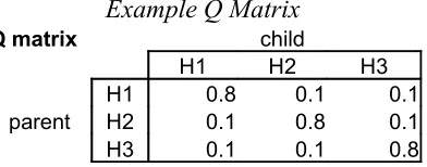
If the agent in one generation has hypothesis 1, then what’s the probability that the agent in the next generation will have hypothesis 1, 2, or 3? These probabilities are displayed in the transition matrix (or Q matrix). In the example Q matrix below (Table 2.2), when an (parent) agent in one generation produces data from H1, then the probability that that data will lead the (child) agent of the next generation to choose H1 is 80%. Since parent H1 can produce data that best supports H2 or H3, then “miscommunications” occur, leading the child to induce H2 or H3 each 10% of the time.

Example Q Matrix

Q matrix child

H1 H2 H3

H1 0.8 0.1 0.1

parent H2 0.1 0.8 0.1

H3 0.1 0.1 0.8

Table 2.2

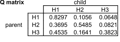
Analytical Q matrix for Sampler with bottleneck of 1:

The following will show the analytical calculation of the Q matrix for a Sampler model with a bottleneck of 1 data sample per generation. All calculations in this section will use the following prior and data likelihood values:

Data Likelihoods

Priors data 1 data 2 data 3

hypothesis 1 0.7 hypothesis 1 0.8 0.1 0.1

hypothesis 2 0.2 hypothesis 2 0.1 0.8 0.1

Table 2.3

Prior and data likelihood values used for all calculations in section 2.2.2

Beginning with cell (H1, H1), we want to know how often parent H1 will produce each possible data string, and how often each of those data strings will lead to the child choosing H1. For a bottleneck of 1, there are just three possible data strings: [1] [2] and [3]. As defined by the data likelihood values of each hypothesis, a parent with H1 will produce d1 with p = 0.8, d2 with p = 0.1, and d3 with p = 0.1. Next, the probability that the child will choose H1 from each of the three data points is defined by the child’s computed posteriors (table 2.4) and their hypothesis choice strategy, sampling. All posterior probabilities are computed with Bayes’ rule as outlined in section 2.1.4.

Posterior Values

H1 H2 H3

[1] 0.9492 0.0339 0.0169 [2] 0.2917 0.6667 0.0417 [3] 0.4118 0.1176 0.4706

Table 2.4

Therefore, when the sampler receives data string [1], it will choose H1 with p = .95, H2 with p = .03, and H3 with p = 0.02. To find out how often parent H1 will lead to child H1, we must multiply the probability that each data string leads to child H1 by the likelihood of that data string being generated by parent H1. Thus, the probability of parent H1 leading to child H1 is (0.9492*0.8) + (0.2917*0.1) + (0.4118*0.1) = 0.8297

Q matrix child

H1 H2 H3

H1 0.8297 0.1056 0.0648 parent H2 0.3695 0.5485 0.0821 H3 0.4535 0.1641 0.3823

Table 2.5

Analytically-calculated Q-matrix for Sampler with bottleneck of 1

Q matrix child

H1 H2 H3

H1 0.8231 0.1102 0.0667 parent H2 0.3685 0.5422 0.0893 H3 0.4539 0.1665 0.3796

Table 2.6

Experimentally-calculated Q-matrix for Sampler with bottleneck of 1

Experimental Q matrix for Sampler with bottleneck of 1:

10,000 runs. As evidenced in this comparison, and other trial calculations, this method of experimentally calculating the Q matrix reliably approximates the analytical solution.

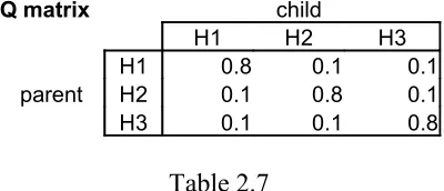
Analytical Q matrix for MAP with bottleneck of 1:

All the steps above for the Sampler are the same for the Maximizer (MAP) except for the way the posteriors enter the equation. As opposed to the samplers, which choose their hypotheses with the probability of each hypotheses posterior probability, the MAP simply chooses the hypothesis with the highest posterior probability. Going back to the posteriors (Table 2.4), data string [1] will always lead to H1, [2] will always lead to H2, and [3] will always lead to H3. So, multiplying the probability that the parent produces each data string times the probability it will be induced under each hypotheses, simply yields the data likelihoods as defined by each hypothesis (Table 2.7).

Q matrix child

H1 H2 H3

H1 0.8 0.1 0.1

parent H2 0.1 0.8 0.1

H3 0.1 0.1 0.8

Table 2.7

Analytically-calculated Q-matrix for MAP with bottleneck of 1

Q matrix child

H1 H2 H3

H1 0.8062 0.0948 0.099 parent H2 0.1016 0.7983 0.1001 H3 0.1038 0.0954 0.8008

Table 2.8

Experimentally-calculated Q-matrix for MAP with bottleneck of 1

Experimental Q matrix for MAP with bottleneck of 1:

Again, for comparison, Table 2.8 shows that the experimentally-calculated Q matrix closely approximates the analytical Q matrix.

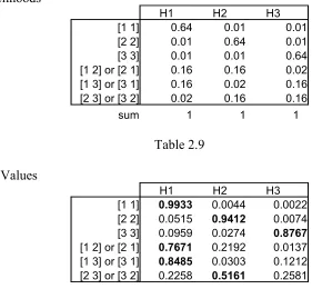
Q matrix calculations for Sampler with bottleneck of 2:

Data Likelihoods

H1 H2 H3

[1 1] 0.64 0.01 0.01

[2 2] 0.01 0.64 0.01

[3 3] 0.01 0.01 0.64

[1 2] or [2 1] 0.16 0.16 0.02 [1 3] or [3 1] 0.16 0.02 0.16 [2 3] or [3 2] 0.02 0.16 0.16

sum 1 1 1

Table 2.9

Posterior Values

H1 H2 H3

[1 1] 0.9933 0.0044 0.0022 [2 2] 0.0515 0.9412 0.0074 [3 3] 0.0959 0.0274 0.8767

[1 2] or [2 1] 0.7671 0.2192 0.0137 [1 3] or [3 1] 0.8485 0.0303 0.1212 [2 3] or [3 2] 0.2258 0.5161 0.2581

Table 2.10

These new likelihoods (Table 2.9) are obtained by multiplying the likelihood values of the data points in question, as defined by each hypothesis (Table 2.3). For example, H1 produces data point 1 with p=.8, so producing it twice has the probability of p=.64. All probabilities in each column sum to one because they cover all possible data strings.

Again, the posterior values (Table 2.10) are computed with Bayes’ rule. When the Sampler receives string [1 1], it will choose H1 with a 99% probability, and H2 and H3 with less than 0.5% probability each. To get each entry of the Q-matrix, all the likelihoods of each string being induced under each hypothesis must be multiplied by the likelihoods that each string is produced at all and then these values are summed. So, for parent H1 going to child H1, this value is the sum of the likelihood that each string is produced by parent H1 times the probability it will be induced as child H1: (.64*.9933)+(.01*.0515)+(.01*.0959)+(.16*.7671)+(.16*.8485)+(.02*.2258) = .9002 Table 2.11 shows the analytical Q matrix and Table 2.12 shows the experimental Q matrix for comparison.

Q matrix child

H1 H2 H3

H1 0.9002 0.0627 0.037 parent H2 0.2197 0.7209 0.0594 H3 0.2591 0.1188 0.6221

Table 2.11

Q matrix child

H1 H2 H3

H1 0.9004 0.0635 0.0361 parent H2 0.2218 0.7178 0.0604 H3 0.2588 0.1166 0.6246

Table 2.12

Experimentally-calculated Q-matrix for Sampler with bottleneck of 2

Q matrix calculations for MAP with bottleneck of 2:

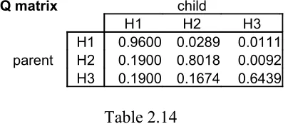
Again, calculations for the MAP differ from the sampler in terms of hypothesis choice. To obtain the analytical Q matrix, only the likelihoods of strings with the maximum posterior will be summed under each hypothesis. These are the values in bold in Table 2.10. Here, strings [1 1], [1 2], [1 3] will always lead to H1. Strings [2 2], [2 3] will always lead to H2, and string [3 3] will always lead to H3. Therefore, the probability that the data from H1 will lead to H1 in the next generation is .64 (for [1 1]) + .16 (for [1 2]) + .16 (for [1 3]) = .96. Table 2.13 is the resulting analytical Q matrix and Table 2.14 is an experimentally-calculated Q matrix for comparison.

Q matrix child

H1 H2 H3

H1 0.96 0.03 0.01

parent H2 0.19 0.80 0.01

H3 0.19 0.17 0.64

Table 2.13

Analytically-calculated Q-matrix for MAP with bottleneck of 2

Q matrix child

H1 H2 H3

H1 0.9600 0.0289 0.0111 parent H2 0.1900 0.8018 0.0092 H3 0.1900 0.1674 0.6439

Table 2.14

Experimentally-calculated Q-matrix for MAP with bottleneck of 2

2.3.3 Analytical and Experimental Stationary Distribution Calculations

The Q matrix summarizes the potential for transition dynamics in the system which it describes. But what can this dynamical fingerprint tell us about the outcome of iterated learning? If an ILM simulation could be run for an infinite amount of time, the relative frequency of each chosen hypothesis would settle into a particular distribution that is determined entirely by the Q matrix. This distribution is known as the stationary distribution and serves as an idealized shorthand for the “outcome of iterated learning.” As demonstrated by Griffiths & Kalish (2005) and Kirby et al. (2007), the stationary distribution is proportional to the first eigenvector of the Q matrix. Therefore, the stationary distribution is easily determined for each model, by normalizing the first eigenvector of its analytically-calculated Q matrix.

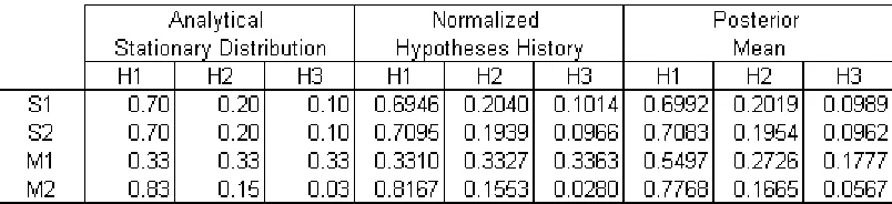
transitions, it represents one actual trajectory of transitions, from a larger set of probable trajectories under that Q matrix. However, when a large number of transitions can be recorded in a simulation (by setting the number of generations sufficiently high), then a tally of the actual hypotheses chosen by the agents over the course of the simulation closely approximates the analytical stationary distribution. Below are the stationary distributions for each of the analytical Q matrices from the previous section (Table 2.15). For comparison, next to each is the normalized hypothesis history of a corresponding simulation run of 10,000 generations. The normalized hypothesis history is a reliable, experimental approximation of the stationary distribution.

Stationary Distribution Approximations

Table 2.15

Normalized Hypothesis History approximates the analytical stationary distribution for both the Sampler and MAP model. The posterior mean is only a reliable approximation for the Sampler model. S1 = Sampler with bottleneck of 1, S2 = Sampler with bottleneck of 2, M1 = MAP with bottleneck of 1, M2 = MAP with bottleneck of 2.

Additionally, for the Sampler only, the average of all agents’ posterior values serve as a good approximation for the stationary distribution. This is because the hypotheses are chosen according to the exact proportions of the posterior vector. For the MAP, posterior mean can not be used as an approximation heuristic. MAP dynamics are not tied to the exact values of the posterior, because agents only respond to the maximum. Table 2.15 shows the posterior mean of the same simulation runs.

2.3.4 Summary

The Bayesian ILM of the present research can be used to experimentally determine the internal dynamics and associated stationary distribution of both Sampler and MAP models, and over a wide variety of parameter combinations. Determining the Q matrices and stationary distributions through experimental calculations and simulation heuristics provide a good alternative to computing the analytical solutions, which becomes increasingly cumbersome as the bottleneck or population size or increases. Additionally, the simulations will allow the investigation of certain parameter combinations, such as multi-agent populations with heterogeneous biases, which do not have straightforward analytical solutions.

2.4 Model Results

previous Bayesian ILMs. Last, it will address new findings for multi-agent populations with heterogeneous and homogeneous biases.

2.4.1 Basic Sampler Behavior of 1-agent, 1-sample simulations

Griffiths & Kalish (2005) showed that the stationary distribution of the Sampler always mirrors the prior. This was confirmed in our model for a 1-agent population. Over all combinations of priors and hypotheses structures tested, the Sampler model’s stationary distribution mirrored the prior. However, this was not the case for multi-agent populations, and will be addressed in section 2.4.4.

2.4.2 Basic MAP Behavior of 1-agent, 1-sample simulations

Kalish et al. (2007) find that the MAP’s dynamics are effected by the prior, data likelihoods (aka: hypothesis structure), and noise. However, it is not understood exactly how the likelihoods affect the dynamics. Because our model does not investigate the effect of noise on the model’s behavior, it is more readily apparent which aspects of the dynamics are due to the prior and which are due to the hypothesis structure. The following explanations of MAP behavior in terms of hypotheses structure and bias influence are novel and were informed by simulations with the present model.

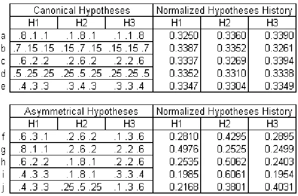
From the Q matrix calculations in the previous section, it is clear that the Q matrix values of a 1-sample simulation are the data likelihood values for each hypothesis. This leads to consistent patterns in the stationary distribution for particular types of hypotheses structures. Overall, the hypotheses structures investigated in this model can be broken down into two main categories; canonical and asymmetrical. Canonical hypotheses structures are ones where each hypothesis is defined by the same set of data likelihood values, but shifted so that each hypothesis’ peak is over a different data point. Examples of canonical hypotheses are in Table 2.16, a-e. Within a canonical hypotheses structure, each hypothesis has identical probabilities of transitioning to every other hypothesis and therefore, when there is no prior bias, each hypothesis is equally represented in the stationary distribution.

Asymmetrical hypotheses structure occurs when each of the hypotheses are not composed of the same values, and therefore have more complex transition probabilities among themselves. Examples of asymmetrical hypotheses are in Table 2.16, f-j. Figure 2.1 is also an asymmetrical hypotheses structure. The stationary distributions of this category of hypotheses are difficult to predict, however we have identified some general trends in the dynamics. Though, these trends may only hold for this particular model’s implementation, with an equal number of hypotheses as data points. The first concerns their relative peak height . The hypothesis with the highest peak likelihood value will be represented with the highest proportion in the stationary distribution. Likewise, the hypothesis with the lowest peak will be represented the least. The second concerns their relative overlap. When all hypotheses have peaks with equal likelihood values, but one has higher extreme likelihoods than the two hypotheses, as does H2 in example f, it will be represented with the greatest proportion in the stationary distribution. These relationships regarding hypothesis overlap and relative likelihood values probably have straightforward analytical solutions and are open points for further analyses.

Table 2.16

Differences in normalized hypothesis history for the two categories of hypotheses; canonical and asymmetrical. All results above were calculated with an unbiased prior.

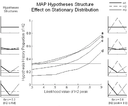
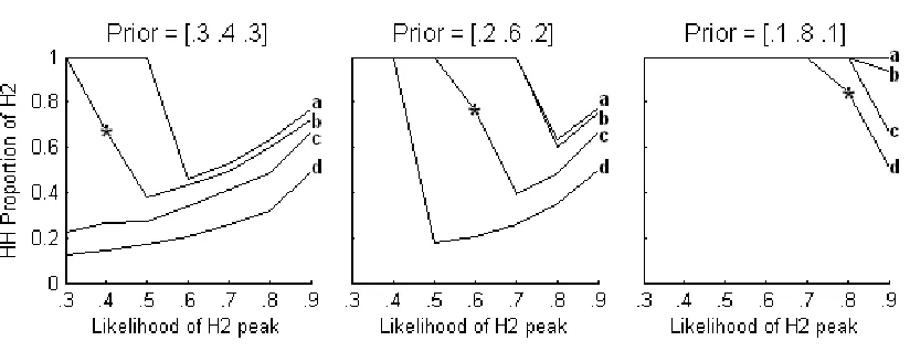
Because these relationships have to do with the entire hypotheses structure, the effect that one hypothesis’ likelihoods has on the stationary distribution always depends on its context, which is the other two hypotheses. This makes for a difficult analysis. Figure 2.2 shows the manipulation of just one hypothesis, H2, in 4 different contexts, and with an unbiased prior. Here, H2’s peak is slowly raised from likelihood value 0.33 (flat/no peak) to 0.9, as shown on the x-axis. The context hypotheses structures are displayed in the columns of graphs at the sides (these graphs display the hypotheses structure as introduced in Figure 2.1). The left column shows a snapshot of the hypotheses structure in order for lines a-d at x = 0.3. The right column shows the structures at x = 0.9. For a, H1 and H3’s peaks = 0.33 (flat), b peaks = 0.4, c

Figure 2.2

Proportion of H2 in the MAP stationary distribution as a function of H2’s hypothesis peak in 4 different hypotheses structures. Peaks of context hypotheses H1 & H3 in a = 0.33 (flat), b = 0.4, c = 0.6, d = 0.8. Prior is unbiased.

Figure 2.3

Hypotheses structure effect on the MAP stationary distribution, with added effects from prior biases.

Table 2.17 directly visualizes this threshold for line c (hypotheses = [.6 .2 .2; .2 .6 .2; .2 .2 .6] of the middle graph in Figure 2.3. Here, the posterior values are given for all possible data strings [1], [2], and [3]. The location of the maximum posterior values (in bold) are what determine the MAP hypothesis choice. Across this threshold, these posterior maxima make a shift, thus shifting the outcome of iterated learning for this model. When the prior value is anywhere lower than the H2 peak, as in prior = [.205 .59 .205], the dynamics remain completely determined by the hypotheses structure. However, nudging the prior up to [.2 .6 .2], which is the same level of the H2 peak, the posteriors move to favor H2 because the MAP is now faced with 2 maximum posterior values for 2 of the data strings and will choose them each 50% of the time. Finally, as soon as the prior bias for H2 exceeds the H2 likelihood peak, as in [.195 .61 .195], all posterior maxima are located under H2. At this point, all agents in the simulation will choose H2 for all possible data strings.

Posterior values under different priors

data Prior = [.205 .59 .205] Prior = [.2 .6 .2] Prior = [.195 .61 .195]

string H1 H2 H3 H1 H2 H3 H1 H2 H3

[1] 0.44 0.42 0.15 0.43 0.43 0.14 0.42 0.44 0.14

[2] 0.09 0.81 0.09 0.09 0.82 0.09 0.09 0.82 0.09

[3] 0.15 0.42 0.44 0.14 0.43 0.43 0.14 0.44 0.42

Table 2.17 Hypotheses = [.6 .2 .2; .2 .6 .2; .2 .2 .6]

Basic Sampler vs. Maximizer Conclusion:

hypotheses structure is canonical, then the probability of an agent choosing any given hypothesis in the stationary distribution is equal. When the hypotheses structure is of various, asymmetrical combinations, the stationary distribution reflects each of them differently. A prior bias adds yet more to the MAP dynamics, but only when it is stronger than the likelihood values.

2.4.3 The Bottleneck Effect

The number of data points that are transmitted between generations constitute the learning bottleneck. The bottleneck size, therefore, equals the number of data samples in the data string. Varying the bottleneck size directly effects the transmission dynamics. When the bottleneck is large, there is a much higher probability that the proportion of data samples in the data string faithfully reflects the likelihoods of hypothesis it was generated from. This leads to greater fidelity of transmission; where each generation usually chooses the same hypothesis as the generation before it. When very little data is transmitted over each generation, transmission fidelity is much lower, yielding many transitions between hypothesis choices within the simulation run. Transmission fidelity is directly visible in the diagonal axis of the Q matrix. A high probability of each hypothesis leading to itself equals high transmission fidelity and a lower number of transitions in the simulation run. As the bottleneck increases, transmission fidelity increases until it reaches 100% and Q matrix diagonals are all equal to 1. Depending on the strength of the bias and the distinctiveness of the hypothesis peaks, this increase occurs at different speeds (Figure 2.4). However, this rate does not seem to be affected by hypothesis choice strategy. All models will eventually reach 100% transmission fidelity at a certain bottleneck size.

Figure 2.4

Increase in transmission fidelity is slower for models with weak biases and likelihoods. Behavior is more determined more by these factors than by hypothesis choice strategy.

Strong: prior = [.7 .2 .1] and hypotheses = [.8 .1 .1; .1 .8 .1; .1 .1 .8] Weak: prior = unbiased and hypothesis = [.4 .3 .3; .3 .4 .3; .3 .3 .4]

For a finite number of generations, all simulations will appear to display complete transmission fidelity when the bottleneck is wide enough. This will occur when the probability of miscommunications (non-diagonal cell values) make it unlikely that they will appear within the given number of generations. For example, if one particular miscommunication has a probability of 0.01, it will usually not occur in a simulation of with less than 100 generations, but it likely to occur several times in a simulation of 10,000 generations.

Bottleneck effect differences between MAP and Sampler:

For both the MAP and Sampler, transmission fidelity increases as the bottleneck widens. The Sampler’s stationary distribution continues to mirror the prior, over all bottleneck sizes and priors tested. This confirms that the bottleneck has no effect on the outcome of iterated learning for the Sampler model. However, it does effect the internal dynamics of transmission and may well have an effect on the outcome of iterated learning over finite time spans. The MAP’s stationary distribution, on the other hand, continues to be affected both by the likelihoods and priors, but changes non-monotonically as the bottleneck widens. Though the MAP’s transmission fidelity steadily increases, the dynamics reflected by the stationary distribution are surprisingly unstable (Figure 2.5). Interestingly, this instability only occurs with asymmetrical hypotheses structures, where the slightest asymmetry leads to wildly different stationary distributions for each bottleneck size. For canonical hypotheses structures, all hypotheses continue to be equally represented in the stationary distribution. Unfortunately, the cause of this strange behavior has not been obtained.

Figure 2.5

MAP posteriors non-monotonically vary as bottleneck widens. The y-axis shows the proportion of H2 in the experimentally-calculated stationary distribution (normalized hypothesis history). Prior = unbiased, Canonical Hypotheses = [.6 .2 .2; .2 .6 .2; .2 .2 .6], Asymmetrical Hypotheses = [.6 .3 .1; .2 .6 .2; .1 .3 .6]

Bottleneck and data variance issues:

the stationary distribution, and transmission fidelity would have no effect. However this is impossible. For all of the data in the present report, all simulations were run for 10,000 generations. At this setting, variance begins to become a problem with Q matrix and stationary distribution approximation around a bottleneck of 6-10. Above this level, multiple runs must be averaged to gain a more complete picture of the model’s dynamics.

2.4.4 Population Size

When the population consists of multiple agents, which dynamics found in the single-agent models hold, and which do not? And what is the outcome of iterated learning when this population has heterogeneous biases? The remaining sections will answer, in terms of this model, these new questions regarding population size and heterogeneity.

In this model, each agent in a multi-agent population sees the same data string, separately calculates their posterior values, chooses their own hypothesis, and generates their own data. The data from each agent of the same generation are then concatenated into one unified data string, which is given to the next generation as their input. When the population parameter is set to any number x, all generations have x population members. When the number of data samples is set to y, each agent in the population produces y number of data samples, yielding a bottleneck size of

x*y.

Normalized Hypothesis History

MAP

H1 H2 H3

samples = 4 0.6352 0.2488 0.1160 population = 4 0.6304 0.2561 0.1135

Sampler

H1 H2 H3

samples = 4 0.6977 0.1918 0.1105 population = 4 0.8104 0.1254 0.0642

Table 2.18

Population size does not add new dynamics for MAP, but for Samplers it does – the stationary distribution no longer mirrors the prior. Prior [.7 .2 .1], hypotheses [.8 .1 .1; .1 .8 .1; .1 .1 .8], 10,000 generations.

Hypotheses Choice of Multi-agent Sampler vs. MAP

Sampler MAP

H1 H2 H3 H1 H2 H3

Hypotheses agent 1 7609 1579 812 8234 1496 270

Chosen agent 2 7674 1570 756 8234 1496 270

Table 2.19

MAP agents choose the same hypothesis, whereas Samplers do not. Prior [.7 .2 .1], hypotheses [.8 .1 .1; .1 .8 .1; .1 .1 .8], 10,000 generations.

For a homogeneous, multi-agent Sampler model, the dynamics are markedly different. Because samplers choose their hypotheses weighted by their posteriors, a homogenous population will not choose the same hypotheses each generation (Table 2.19). Therefore, the data samples do not come from the same set of likelihood values. This has interesting implications concerning the perfect Bayesian rationality of the agents. In the case of the MAP, the agents have all the possible sets of likelihoods that the data could be generated from, already given to them as their hypotheses. When a string of data is generated from a set of likelihoods which the agents are not explicitly given, then they are not longer perfect Bayesian reasoners. This is exactly the case with a multi-population of Samplers. When a data string in generated from 2 different hypotheses, these probabilities do not conform to the likelihoods as defined by any of their hypotheses. The result is, for a multi-population of Samplers, the stationary distribution no longer mirrors the prior (Figure 2.6).

Figure 2.6

The MAP model’s stationary distribution is invariant to population size. For Samplers, population size does affect the dynamics and the stationary distribution no longer mirrors the prior. Stationary distributions for populations 1 and 2, for MAP and Sampler models with: prior [.7 .2 .1], hypotheses [.8 .1 .1; .1 .8 .1; .1 .1 .8], 10,000 generations.

Additionally, some systematic variance was observed for the multi-agent Sampler model in regard to manipulations of the likelihood structure. Figure 2.7 shows that the stationary distribution mirrors the prior less and less as the hypotheses structure becomes strongly peaked and the prior more biased. However, for a combination of relatively flat hypotheses and weakly biased priors, the stationary distribution still mirrors the prior. Additionally, increasing the population size systematically amplifies the effect of the likelihoods on the Sampler’s stationary distribution (Figure 2.8).

Figure 2.7

Strong biases and peaked hypotheses lead the sampler away from converging to the prior.. a = prior [.3 .3 .3] b = prior [.6 .2 .2] c = prior [.7 .2 .1] d = prior [.8 .1 .1], Population = 2.

Figure 2.8

2.4.5 Heterogeneity

A heterogeneous ILM was implemented by taking a multi-agent model and assigning different prior vectors to each of the agents. This model, therefore, is the most complex of all models constructed. For this reason, only 2-agent heterogeneous populations will be used as examples in this section.

The main result is that heterogeneous agents’ hypotheses choices converge as they are allowed to share more and more data, despite having fixed and different priors from each other (Figure 2.10 and 2.12). This conforms to the general tradeoff between the likelihoods and prior in Bayesian induction; the more data that is seen, the less the effect of the prior on the posterior distribution over hypotheses. Because the behavior of both models is based on the posterior values, increasing the amount of data which the agents share produces increasingly similar posterior values, despite differences in agents’ priors. In the following analyses, convergence is measured by the Euclidean distance between each agent’s normalized hypotheses history vector.

Since agents’ behavior is converging, the natural question is, to what? To structure this question more, we decided to investigate whether or not the converged behavior of a heterogeneous ILM (where agent x and agent y each differ in their prior bias) is just an average of the behavior of one homogeneous run with agent x and one with agent y. It turns out, this is not a simple question. First, it is difficult to determine exactly what the true average of agent x and agent y’s behavior is, due to the variation among runs inherent in the simulation. Additionally, as discussed previously, the stationary distribution of a particular model changes as a function of bottleneck or population size. Therefore, we cannot just average the stationary distribution of agent

x and agent y for comparison to a 2-agent simulation composed of agent x and agent y. Instead, we should match for the number of samples in the data string. For the Sampler, it is established that manipulating bottleneck size does not effect the stationary distribution: it will continue to mirror the prior. However, manipulating the population size slightly effects the stationary distribution away from mirroring the prior. Although, this effect isn’t noticeable at a population of 2 for relatively flat hypotheses and a mildly biased prior. Therefore, the average behavior for Sampler agent x and Sampler agent y can be done with some confidence – by just averaging the priors of the two agents – but only when hypotheses are relatively flat and the bias is weak.

Heterogeneous Sampler behavior:

Looking at the last reliable run from Figure 2.9, at bottleneck 16, the normalized hypotheses history of each agent are displayed in Table 2.20. Here, it is clear that the convergence behavior is settling around the average of both agent’s priors.

Average of Converging Behavior

H1 H2 H3

agent 1 0.43 0.21 0.36

agent 2 0.37 0.21 0.42 Average of both Priors

average 0.40 0.21 0.39 0.4 0.2 0.4

Table 2.20

Hypotheses History of each agent at bottleneck = 16, from Figure 2.9, and the average of their priors.

Figure 2.9

Figure 2.10

Euclidean distance between the agents’ hypotheses histories, of which H1 is graphed in Figure 2.9.

In section 2.4.4 we discussed some parameter combinations, for the multi-agent Sampler, which did not result in a stationary distribution that mirrored the prior. Namely, strongly-peaked hypotheses structures plus strong biases. Some of these combinations were also analyzed in the heterogeneous model, however, the normal variance of each run subsumed the difference between the averaged priors and the average outcome of the multi-agent runs which did not mirror the prior. Therefore, it is impossible to determine a difference in convergence when comparing these two conditions.

Heterogeneous MAP behavior:

As we’ve demonstrated in previous sections, the dynamics of the MAP model are more complex than that of the Sampler, and the heterogeneous models are no exception. The MAP model behaves very differently over an increasing bottleneck depending on whether the hypotheses structure is canonical or asymmetrical (refer back to Figure 2.5). Due to the unexplained, non-monotonic variance over bottleneck size of MAP models with asymmetrical hypotheses, we will restrict the heterogeneous MAP analyses to canonical hypotheses structures.

distribution for single-agent, bottleneck = 2 model for agent 1 is [.83 .15 .03] and agent 2 is [.03 .15 .83]. The average of these vectors is [.43 .15 .43]. However, the hypothesis history of the heterogeneous model does not settle upon this average. Due to the variation over runs, it is difficult to determine what the actual convergence state is. However, it seems that the heterogeneous model is converging somewhere off of this average, rather then homing in on it as the Sampler model did.

Figure 2.12 shows some additional simulations, where each graph shows a simulation with a different set of agent priors. These also seems to converge somewhere off of the trivial average. Recall that MAP stationary distributions are differentially sensitive to whether the maximum prior value is higher or lower than the maximum hypotheses peak value (refer back to Figure 2.3). This differential sensitivity is also confirmed in the heterogeneous MAP model. In figure 2.12 and 2.13, models (a) and (b) have a bias which exceeds the maximum likelihood values of the hypothesis structure, whereas the bias in models (c) and (d) do not. The convergence behavior for these two sets of models are qualitatively different.

Figure 2.11

Figure 2.12

MAP convergence for 4 simulations, each where agents have a different set of priors. a-d: Hypotheses = [.6 .2 .2; .2 .6 .2; .2 .2 .6], a: prior agent 1 = [.4 .3 .3] and prior agent 2 = [.3 .3 .4], b: prior agent 1 = [.59 .205 .205] and prior agent 2 = [.205 .205 .59], c: prior agent 1 = [.6 .2 .2] and prior agent 2 = [.2 .2 .6], d: prior agent 1 = [.8 .1 .1] and prior agent 2 = [.1 .1 .8]

Figure 2.13

Summary Heterogeneous ILM:

For both the MAP and Sampler models, the behavior of 2 agents with heterogeneous biases converges as a function of the bottleneck size. The more agent’s share each other’s data, the more they choose the same hypotheses as each other. At very large bottlenecks, agents choose the exact same hypothesis throughout the simulation, showing that a sufficiently strong data likelihood value can override agent’s differences in prior biases. However, the inherent variance of a finite simulation over high bottlenecks, makes it impossible to obtain an exact distribution of hypotheses that is being converged to. It appears that the Sampler model tends toward convergence to a trivial average of the agents’ priors. The MAP model seems to converge slightly below this level. However, overall the behavior of the Sampler and the MAP in the heterogeneous model are qualitatively very similar. we’ve probably shied away from addressing the true complexity of convergence by limiting myself to 2-agent, bottleneck = 2 simulations, canonical hypotheses structures, and symmetrical prior sets. Undoubtedly, such simulations will yield more variance in behavior according to more fine-grained categories of parameter settings. However, these simulations are only a first step in addressing bias heterogeneity in a Bayesian ILM.

2.5 Model Discussion

This Bayesian ILM both replicated the general properties of previous existing Bayesian ILMs and provided new results regarding multi-agent populations and bias heterogeneity. The replications are that a single-agent Sampler model’s stationary distribution always mirrors the prior bias of the agent (Griffiths & Kalish, 2005), and a MAP model’s stationary distribution is determined both by the prior and the data likelihood values (Kalish et al., 2007). Also, for a range of parameters, the prior has no effect on the MAP stationary distribution (Smith & Kirby, 2008?), but above this threshold, iterated learning amplifies this bias (Kirby et al., 2007). Additionally, a strong bottleneck effect was observed, with the general effect of increasing transmission fidelity of both the Sampler and MAP models (Kalish et al., 2007). Last to note, the normalized history of all hypotheses choices over the course of the simulation yielded the same solution as analytically calculating the Q matrix, as in Nowak et al. 2001. All of these replications attest to this particular implementation as a valid Bayesian iterated learning model.

Throughout the replication work, new insights into the role of data likelihoods for both the MAP and Sampler were obtained. The focus of all previous research with Bayesian ILMs is the on prior and how its manipulations affect the stationary distribution. Kalish et al. (2007) manipulated the degree of hypotheses overlap, as well as noise level, but it appears their hypotheses correspond to what we call the canonical form in our analyses. Otherwise, the rest of the literature does not manipulate the data likelihoods of their model. My analyses of both canonical and asymmetrical hypotheses structure, and in the absence of noise, sheds new light on

in the case of asymmetrical hypotheses, this sensitivity to the bottleneck is surprisingly unstable.

The results of Smith & Kirby (2008) demonstrate that the MAP strategy of hypothesis choice is evolutionarily stable over that of samplers. However, the MAP parameters for which this result was proven, it seems, were derived from a canonical hypotheses structure and for the range of priors which are unaffected by bias strength (refer back to Figure 2.3). The result is consistent behavior of the Smith & Kirby’s MAP model over the bias values they selected. My results show that this is a subset of MAP behavior and that unstable behavior is easily obtained for the right relationship between hypotheses and priors. So, perhaps MAP would not be the evolutionary stable strategy in all cases. Or additionally, perhaps it can be shown that a certain range of MAP parameters is evolutionary stable over other MAP parameter sets. Knowledge of this kind would help guide the right choice of MAP parameter sets to use for iterated learning simulations, rather than convention (i.e. assuming one un-manipulated set of canonical hypotheses).

Another novel result was obtained from a manipulation in population size. By just increasing the population size to 2, the Sampler model’s stationary distribution does not strictly mirror the prior. The result is that the hypothesis with the highest prior becomes amplified in the stationary distribution, and some sensitivity to the likelihood structure emerges. This result is due to the fact that Samplers, according to this model’s multi-agent implementation, can no longer be classified as perfect Bayesian reasoners (refer back to section 2.4.4).

The population manipulation was also informative in terms of this paper’ ultimate question; what does cultural transmission add? Since population size, in part, defines the social structure and transmission dynamics of an ILM, any manipulation to population size that affects the stationary distribution can be taken as evidence for cultural transmission “adding” something. Referring back to Figure 2.6, it is clear that cultural transmission adds additional dynamics in the case of the Sampler, but not in the MAP. Interestingly enough, the existing literature claims the reverse: cultural transmission adds nothing to the Sampler model, but does to the MAP model.