Modelling of the behaviour of a welded joint subjected to reverse bending moment at high temperature

Modelling of the Behaviour of a Welded Joint subjected to Reverse Bending Moment at High

Temperature

Alan R. S. Ponter and Haofeng Chen

Department of Engineering, University of Leicester, Leicester, LE1 7RH, UK e-mail: asp@le.ac.uk ,Tel UK+1162522549, Fax UK+1162522525

Abstract.

Background. The paper is concerned with the modelling of the behaviour of welds when subjected to severe thermal and mechanical loads where the maximum temperature during dwell periods lies in the creep range. The methodology of the Life

Assessment Method R5 is applied where the detailed calculations are carried out using the Linear Matching Method, with the

objective of generating an analytic model.

Method of Approach. The Linear Matching Method (LMM) has been developed to allow accurate predictions using the methodology of R5, the UK Life Assessment Method. The method is here applied to a set of weld endurance tests, where reverse

bending is interrupted by creep dwell periods. The weld and parent material are both Type 316L(N) material and data was

available for fatigue tests and tests with 1hr and 5hr dwell periods to failure. The elastic, plastic and creep behaviour of the weld

geometry is predicted using the LMM using the best available understanding of the properties of the weld and parent material.

The numerical results are translated into a semi-analytic model. Using the R5 standard creep/fatigue model, the predicted life of

the experimental welds specimens are compared with experimental data.

Results. The analysis shows that the most severe conditions occur at the weld/parent material interface, with fatigue damage predominantly concentrated in the parent material, whereas the creep damage occurs predominantly in the weld material. Hence

creep and fatigue damage proceed relatively independently. The predictions of the model are good, except that the reduction in

fatigue life due to the presence of the weld is underestimated. This is attributed to the lack of separate fatigue date for the weld

and parent material and the lack of information concerning the heat affected zone. With an adjustment of a single factor in model,

the predictions are very good.

Conclusion. The analysis in this paper demonstrates that the primary properties of weld structures may be understood through a number of structural parameters, defined by cyclic analysis using the Linear Matching method and through the choice of

appropriate material data. The physical assumptions adopted conform to those of the R5 Life Assessment Procedure. The

resulting semi-analytic model provides a more secure method for extrapolation of experimental data than previously available.

1. Introduction

In the design and life assessment of structures of austenitic steels that operate at high temperatures, the performance of welds

design codes have taken welded joints into account by assigning increased factors of safety on allowable loads and temperatures

compared with the factors that apply when welds are absent. These factors are determined from experimental data and experience

in practice. When high temperature failures occur, there is a high probability that the failure will initiate at a weld. The practice of

increased factors of safety discourages designers from allowing a weld to become the primary carrier of load, but in many

circumstances the need to ensure welds are subjected to sufficiently low loads can dominate the overall design.

There is an urgent need to understand the various factors that effect weld strength. In this paper we are concerned with the effect

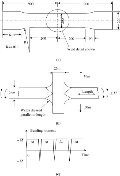
of variable load at high temperature. The problem under consideration is shown schematically in Figs. 1(a) and 1(b). A

continuous plate is divided, at its centre, into two parts each of which is welded to the surface of a third plate. Hence the weld

joint consists of two symmetrically placed identical welds. The simplest description of a typical weld subdivides the material into

three regions, the parent material, assumed uniform away from the weld, the weld material and a thin layer, the heat effected zone

(HAZ), between the weld and parent material. Each of these regions would be expected to have separate material properties.

Differences in elastic properties induce local stress raisers at the interfaces; differences in plastic deformation properties combine

with the elastic properties to produce local plastic strain concentrations. During dwell periods, differences in the creep

deformation properties as well as elastic properties will influence the location and magnitude of creep strain produced during

stress relaxation. The ultimate failure of the component then depends upon the fatigue and creep damage properties which, again,

will vary between the three component materials.

In modelling this situation the objective must be to gain an understanding of the relationship between possible variations in the

material within the weld and the lifetime of the component for a practical range of load variation and dwell time. There are two

difficulties in successfully completely such an analysis; the material behaviour may not be well understood and the analysis

required is very demanding. In the following we concentrate upon a geometry and loading history for which experimental data

exists, Bretherton et al [1,2], making use of a range of data for this particular material, Type 316L(N) austenitic stainless steel.

For analysis we use methods based upon the Linear Matching Method that have already been developed for creep/fatigue

interaction applications in the UK life assessment method R5, Chen and Ponter [3-8]. This allows the development of a model

that may be directly compared with tests conducted on welds and, at the same time, provides insight into the sensitivity of the life

upon material and loading parameters.

The assumptions in the analysis are very simple. Plastic strains are modelled by a Ramberg-Osgood expression. Creep is

modelled by a time hardening law. Failure assumes a linear summation of fatigue damage and creep damage. Creep damage is

modelled as strain exhaustion. There is no interaction between creep strain and plastic strain. Our main objective is to obtain, for

this particular weld geometry, a semi-analytic model of failure that may be developed for other geometries, material data and

2.

The Cruciform Weld Specimen

The geometry of the weld specimen is shown in Figs, (1a) and (1b), where a plate of width 200mm and length of 1.8m is divide

and welded to plate of length 100mm, as shown in Fig. (1b), forming a cruciform specimen. The arms of the specimen are

subjected to a bending moment history, Fig. (1c), consisting of a rapid reversal of bending moment of magnitude

Δ

M

=

2

M

separated by dwell periods of length

Δ

t

when the moment is maintained constant at

M

=

M

=

Δ

M

/

2

. The geometry of the welds is shown in Fig. (1b). A number of experiments had been carried out on such specimens made of 316N(L) austenitic

stainless steel at a constant temperature of

550

o

C

by Bretherton et al [1,2] and for various values of

M

and

Δ

t

, details of which are described below. The analysis described below was conducted to characterise the steady state response of these

specimens and the initiation of failure; the material data used is discussed in the next section.

3. Material

Description

The total strain was assumed to consist of the sum of elastic, plastic and creep components,

c ij p ij e ij

ij

ε

ε

ε

ε

=

+

+

(1)

where the elastic component

ε

ijewas characterised by Young’s modulus E and Poisson’s ratio ν . For the plastic component, two

separate descriptions were used. For the evaluation of standard structural strength parameters such as limit, shakedown and

ratchet limits, a perfectly plastic model was used with a von Mises yield condition and yield stress

σ

y. For the evaluation of the

amplitude of plastic strain, a Ramberg-Osgood expression was used between the plastic strain amplitude

Δ

ε

_ijpand stress

amplitude

Δ

σ

_ij,

ij p p

ij

ε

σ

σ

ε

Δ

Δ

Δ

=

Δ

2

3

,

ε

σ

β 1

2

2

⎟

⎠

⎞

⎜

⎝

⎛ Δ

=

Δ

A

p

(2)

where

Δ

σ

=

σ

(

Δ

σ

_ij

)

and

(

ijp

)

p

ε

ε

ε

=

Δ

Δ

and

(

σ

,

ε

)

refer to von Mises effective values. The two plasticity models are

related by defining the yield stress as half the stress range that results from a strain range of 0.2% in the steady state;

β

ε

σ

σ

_⎟⎟

⎠

⎞

⎜⎜

⎝

⎛ Δ

=

Δ

=

2

2

% 2 .

0 p

y

A

,

Δ

ε

p

=

0

.

2

%

(3)

Table 1 lists the material parameters for 316N(L) austenitic stainless steel at

550

o

C

for the parent, weld and heat affected zone. The Ramberg-Osgood parameters are measured from tests taken to failure and three sets of values are listed here, from the first

For the evaluation of the creep properties, separate relations were available for primary and secondary creep at

550

o

C

. The primary uniaxial creep was give by the Norton-Bailey equation,

18 . 4 42131 . 0 15

10

9618

.

2

σ

ε

_cr

=

×

−

t

(4)

where time t is in hours and stress in MPa. Hence the primary creep strain rate may be calculated by:

18 . 4 57869 . 0 15

10

2478

.

1

σ

ε

₌

_×

− −

t

cr

&

(5)

The time at the end of primary creep was determined by

t

=

4

.

4926

×

10

19

σ

−6.9467. For secondary creep, the creep rate is 2

. 8 28

10

29

.

5

σ

ε

₌

_×

−

cr

&

(6)

Based upon the cyclic stress strain data, for both parent and weld materials, semi-total stress range is less than 400MPa when the

semi-total strain range is less than 1%. In the experimental results to be discussed below, the maximum outer fibre total strain

range is 1%. Hence, the maximum cyclic stress at the stress concentration during the hold period is assumed to be no more than

400MPa, the minimum time at the end of primary creep

t

=

4

.

4926

×

10

19

×

400

−6.9467

=

38

hours

. As the hold periods are 1 or 5 hours only primary creep need to be considered for comparison with the test data.

4. Elastic

Analysis

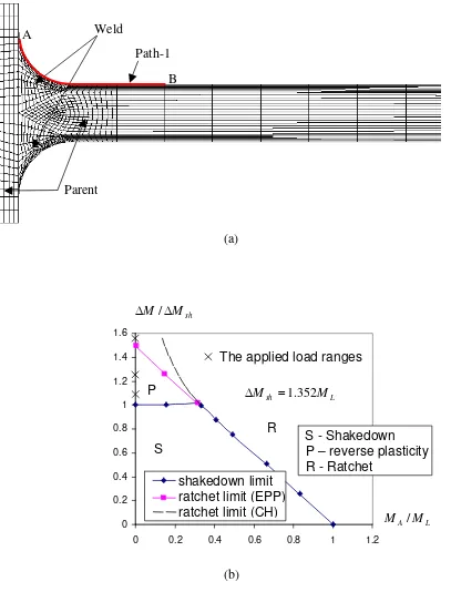
The finite element mesh for a two dimensional symmetric model of the cruciform specimen is shown in Fig. (2a) for the weld and

parent materials. The mesh comprises 8-noded generalised plane strain quadrilateral elements. We find that the inclusion of the

heat affected zone has a negligible effect on the solutions reported here.

5.

Shakedown and Ratchet Limit Analysis

The limit load, shakedown limit and ratchet limit was evaluated for a perfectly plasticity and a von Mises yield condition. The

history of bending moment consisted of a variation between

M

=

M

_A

+

M

and

M

=

M

_A

−

M

, i.e. a variation of

M

M

=

2

Δ

and a constant addition moment

M

A. The analysis was carried out using the Linear Matching Method, Chen and

Ponter [3,4], and the resultant boundaries are shown in the interaction diagram, Fig. (2b), in

(

M

_A

/

M

_L

,

Δ

M

/

Δ

M

_sh

)

space

where

M

L and

Δ

M

shdenote the limit moment and shakedown limit respectively,

kNm

M

_L

=

7

.

438

,

Δ

M

_sh

=

10

.

056

kNm

=

1

.

352

M

_L (7)

The diagram is divided into four regions, shakedown (including elastic) S, Reverse plasticity P, and Ratchetting R. Also included

is the boundary between the P and R regions assuming complete cyclic hardening (CH), Chen and Ponter [4]. For various degrees

(EPP). The

Δ

M

values corresponding to the experimental results are shown as crosses and all lie within the reverse plasticity region.

6.

Steady State Cyclic Plasticity

We first consider the case when creep deformation is ignored and the Ramberg-Osgood equation applies. Again the Linear

Matching Method, Chen and Ponter [4], was used where steady state cyclic hardening solutions are generated. For the case

sh

M

kNm

M

=

=

Δ

Δ

12

.

466

1

.

24

, the variation of

Δ

ε

p

=

ε

(

Δ

ε

_ijp

)

along the path A to B is shown in Fig, (3a). The

maximum plastic strain occurs at the parent/weld interface within the parent material. Within the weld, the plastic strain rapidly

decreases and remains negligible within most of the weld material. At the interface, however, there is a significant strain

concentration factor. The variation of the maximum von Mises stress along AB is shown in Fig. (3b). In this case the maximum

stress occurs at the weld interface within the weld material. This distinction between the position of the maximum strain range (in

the parent material) and the maximum stress (in the weld material), is important in understanding the two modes of damage due to

fatigue and creep and their interaction.

7.

Creep Relaxation during Dwell Period

During the dwell period, stress relaxation occurs as creep strains are substituted for elastic strains. The resulting overall

deformation can only be understood if the interaction between plastic and creep strains occurs. The analysis of such situations has

been discussed by Chen and Ponter [8] and applied to a number of problems, Chen and Ponter [5-8]. Here we adopt the same

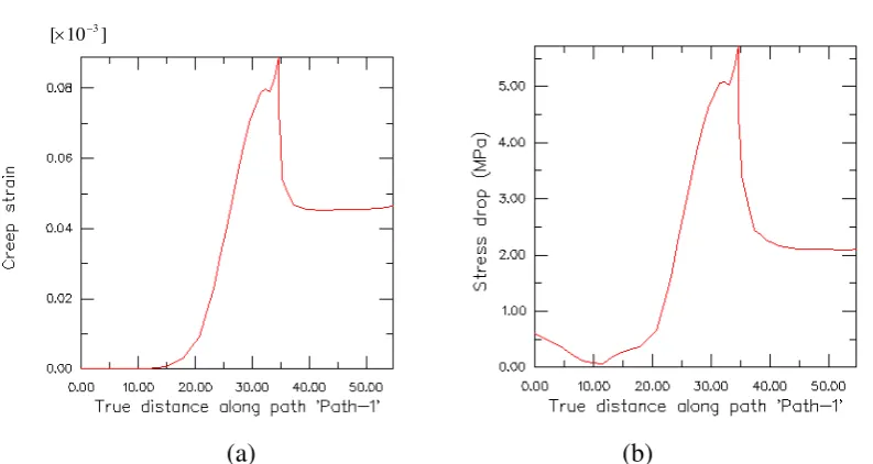
methodology as used in Chen and Ponter [8]. The numerical solutions for dwell periods of both 1hr and 5 hrs show that the creep

strains have a negligible effect on the plastic strain range. Figure (4) shows that the creep strains are small compared with the

plastic strains, Fig.(4a), and the stress drop is small compared with the initial stress, Fig.(4b). The maximum creep strain occurs,

as expected, at the position of maximum stress, i.e. at the weld/parent interface, but within the weld material, and not at the

position of maximum plastic strain. Hence the primary interaction between elastic/plastic and creep strains occurs through the

definition of the maximum stress by the elastic and plastic properties.

An important parameter that governs the interaction between creep and elasticity is the elastic follow-up factor

Z

, defined as

c c

E

Z

σ

ε

Δ

Δ

=

(8)

where

)

1

(

2

3

ν

+

=

E

E

denotes the effective elastic modulus,

Δ

σ

c is the drop in effective stress and

Δ

ε

cis the effective

at either side of the weld/parent interface. It can be seen that the values are sensitive to location but not to dwell time. The

variation with load will be discussed below.

8. Predicted

Lifetimes

On the basis of these deformation based calculations, it is now possible to predict the weld lifetime in terms of the number of

cycles to failure and dwell period. Where comparisons with experimental results are concerned, this presents a difficulty as the

fatigue behaviour of the weld material was not available. The number of cycles to failure

N

_f for tests with no dwell period for

the parent material was expressed in terms of the total strain range

Δ

ε

t in %;

(

)

(

)

2 _{2 3}

1

(

)

(

)

(%)

m

Log

N

m

Log

N

m

Log

Δ

ε

_t

=

_f

+

_f

+

(9)

where, for the parent material,

m

1

=

0

.

085943

,

m

2

=

−

0

.

94691

and

m

3

=

2

.

2274

.

The creep endurance

D

_c, the proportion of the creep ductility exhausted in each cycle, and

N

_c,the number of cycles to failure

due to creep alone, are given by

L c

c

D

ε

ε

Δ

=

,

c c

D

N

=

1

(10)

where, as before,

Δ

ε

cis the accumulated creep strain during relaxation and

ε

_Lis the creep ductility. Again, data was not

available for the weld material. For the parent material we adopt a value of 14%. This represents a minimum value in available

data and is regarded as an appropriate value for weld material. In the absence of data for the weld material, the same data is

adopted for both parent and weld. The estimate of total lifetime, corresponding to crack initiation, is given by a linear summation

of fatigue and creep damage i.e. the total number of cycles to failure

N

₀∗ is given by;

c

f

N

N

N

1

1

1

0

+

=

∗ (11)

As the creep strain is small, its inclusion in the total strain range

Δ

ε

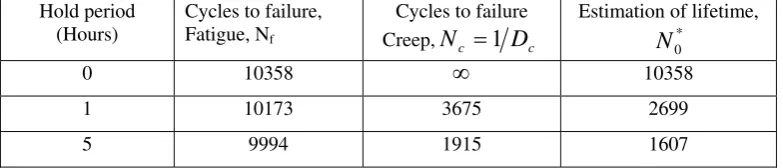
_thas a negligible effect on fatigue damage.

Table 3 and 4 show typical results for

Δ

M

=

1

.

24

Δ

M

_shfor the numbers of cycles to failure evaluated, again, on either side of the weld interface. The load level corresponds to a total strain range of

0

.

5

%

on the outer fibres of the parent material away

from the weld, i.e. at a fairly severe state of loading. There are two notable features of these results. For increasing dwell periods,

creep damage quickly dominates and, for a dwell period of 5hrs, the number of cycles to failure, ignoring fatigue, is close to the

predicted value. At the same time there is a movement of the critical location with increasing dwell time. In the absence of a dwell

the critical point moves to the weld material where the maximum stress occurs. For a 1 hr dwell period,

N

₀∗ is near equal at the

two locations, but for a 5hr dwell period, the critical position is in the weld. As the creep ductility of the weld material is likely to

be less than in the parent material, this implies that failure in the weld with a creep dominated mode is the most likely failure

mode.

In the following section, we develop a simple analytic description of the behaviour of key parameters in the parent material,

remote from the range. This allows a normalisation of the behaviour adjacent to the weld interface as deviations from the remote

behaviour, over a wide range of loads and dwell periods. This forms the basis for a semi-analytic solution to the life of the weld.

9.

Behaviour Remote from the Weld

Consider a beam problem where a section of beam of thickness h and breadth b is subjected to a reversing bending moment of

amplitude

Δ

M

.

Consider the Ramberg-Osgood relationship (1) and (2), repeated here for uniaxial or effective stress and strain,

β

σ

σ

ε

=

Δ

+

(

Δ

)

1

Δ

A

E

(12)

There are two extreme solutions. Consider the case when the plastic strain amplitude is ignored. The maximum linear elastic

stress amplitude is then given by;

M

bh

e

=

Δ

Δ

σ

_max

6

₂ ,

E

e

e max

max

σ

ε

=

Δ

Δ

(13)

The elastic shakedown limit

Δ

M

shRis given by a reverse plasticity limit when

Δ

σ

=

2

σ

y, i.e.

y R

sh

bh

M

σ

3

2

=

Δ

(14)

Comparisons with the LMM solution gives that

Δ

M

sh

=

1

.

015

Δ

M

shR, a 1.5% increase due to the elastic stress concentration at the weld interface.

Another extreme is given by the case when the elastic strain amplitude is negligible and the total strain range is given by the

second term in equ. (12). In this case a simple analytic solution is possible, Ponter and Chen [9]. The solution is best normalised

with respect to a reference plastic strain amplitude

Δ

ε

₀pcorresponding to a stress reference stress amplitude

Δ

σ

₀

=

2

σ

_y where

these quantities are related by

Δ

ε

₀p

=

A

(Δ

σ

₀

)

1β. In the following we will choose

Δ

ε

₀p

=

0

.

2

%

as this corresponds to the definition of

σ

_yused previously. The analytic solution, Ponter and Chen [9], may now be expressed in the following reference

y sh R

M

M

_σ

σ

0

.

6801

2

Δ

Δ

=

Δ

, Rp

p

ε

ε

=

Δ

Δ

_max

1

.

57

(15)

where β β

σ

σ

ε

1 1 0

6801

.

0

%

2

.

0

%

2

.

0

_⎟⎟

⎠

⎞

⎜⎜

⎝

⎛

Δ

Δ

=

⎟⎟

⎠

⎞

⎜⎜

⎝

⎛

Δ

Δ

=

Δ

sh R p R

M

M

(16a)

For the linear elastic solution, corresponding to

β

=

1

, equ. (15) still applies and equ. (16a) is replaced by

E

R e

R

σ

ε

=

Δ

Δ

(16b)

This suggests that a good approximation to the total strain range, in the case when both elastic and plastic terms in equ. (11) are

included, will be given by the combination of equ. (16a) and equ. (16b),

R

ε

ε

=

Δ

Δ

_max

1

.

57

where Rp

e R

R

ε

ε

ε

=

Δ

+

Δ

Δ

(17)

where the individual reference values are given by equ. (16a) and equ. (16b) corresponding to the same reference stress equ. (15).

In Figure (5) we show a comparison between this analytic solution for the plastic strain range and computed values from the

LMM solution for both the remote solution and the solutions at the weld interface for

0

≤

Δ

M

Δ

M

sh

≤

2

and

β

=

0

.

2996

. In Figure (6) we show the variation of the plastic strain amplitude, normalised with respect to the remote amplitude. Hence we see

that the analytic solution equs. (15), (16) and (17) compares well with computed values. At the parent weld interface the

maximum strain concentration occurs close to

Δ

M

/

Δ

M

_sh

=

1

in the parent material. Hence a conservative estimate of the

maximum strain amplitude adjacent to the weld

Δ

ε

W_maxis given by

max max

1

.

30

ε

ε

=

Δ

Δ

W

, in the parent material (18)

The factor 1.30 corresponds to the Fatigue Strength Reduction Factor (FSRF), usually extracted from feature tests conducted on

welds. Here we have derived this value from known elastic and plastic material properties.

For the creep damage calculations we require estimates of the maximum stress, prior to relaxation,

σ

_maxic

=

Δ

σ

_max

/

2

, and values of the elastic follow-up factor Z. Again these can be estimated analytically for the plate remote from the weld. The

following expression is derived by Ponter and Chen [9] for the relationship equ. (12), ignoring elastic strains,

R

σ

β

σ

⎟

Δ

⎠

⎞

⎜

⎝

⎛ +

=

Δ

3

2

015

.

1

max

, _y

Figure (6) shows a comparison between this equation, with

β

=

1

(linear elasticity) and

β

=

0

.

2996

(plastic strains only) with the computed values. The

β

=

1

case coincides with the computed solution for low loads, whereas the slope of the computed solution coincides with the case

β

=

0

.

2996

for

Δ

M

/

Δ

M

_sh

>

0

.

8

. The following solution provides a good approximation in the weld material, over the entire range of load;

⎪⎩

⎪

⎨

⎧

≤

Δ

Δ

Δ

Δ

=

≥

Δ

Δ

⎟⎟

⎠

⎞

⎜⎜

⎝

⎛

₊

−

Δ

Δ

+

=

α

σ

σ

α

β

α

β

σ

σ

sh sh y ic sh sh y ic

M

M

when

M

M

M

M

when

M

M

,

015

.

1

,

3

1

3

2

015

.

1

max

max (20)

where

α

=

0

.

45

. In Figure (8) the initial creep stress is normalised with respect to the remote value. The maximum stress

concentration at the weld occurs in the weld material as expected, for a practical load range, and a simple upper bound is given by

ic icW

max max

1

.

20

σ

σ

=

, in the weld material (21)

10. Estimates of the Elastic Follow-up Factor Z

The value of the elastic follow-up factor Z depends upon the non-linearity of the creep behaviour, i.e. the exponent n, and the

entire initial distribution of stress, governed by the elastic/plastic properties. Close analytic estimates are, in this case, more

difficult to obtain. However a suitable method is given by Ponter and Chen [9] for the case when plastic strains dominate. This

results in the following estimate;

1

2

−

+

=

n

n

Z

β

β

(22)

For low bending moments when elastic strains dominate, the corresponding Z value is given by

n

=

4

.

18

and

β

=

1

, i.e

94

.

1

=

Z

. For high moments, when plastic strain dominate,

n

=

4

.

18

and

β

=

0

.

2996

then

Z

=

12

.

86

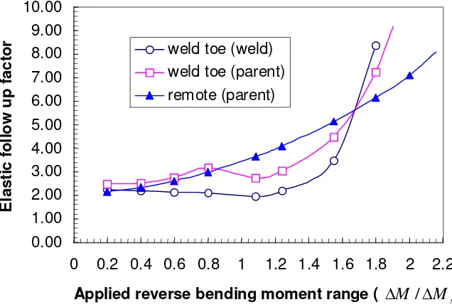
. Hence there is an expectation that Z will vary significantly with load level. The computed values are shown in Fig, (9), computed for a dwell time

of 5hrs, although the value is insensitive to dwell time. The values remote from the weld vary within this predicted range whereas

the values at the weld interface exhibit a rather different mode of behaviour. For low loads Z values are relatively constant and

[image:9.595.65.477.187.269.2]

Weld interface (weld):

Z=2,

<

Δ

Δ

<

sh

M

M

0

1.2 (24a)

3 2

30.68281

+

113.20737

-140.11189

+

-55.98168

_⎟⎟

⎠

⎞

⎜⎜

⎝

⎛

Δ

Δ

⎟⎟

⎠

⎞

⎜⎜

⎝

⎛

Δ

Δ

Δ

Δ

=

sh sh sh

M

M

M

M

M

M

Z

>

1

.

2

Δ

Δ

sh

M

M

(24b)

Weld interface (parent):

Z=3,

<

Δ

Δ

<

sh

M

M

0

1.2 (25a)

3 2

7.87641

+

24.75466

-27.52588

+

-8.04497

_⎟⎟

⎠

⎞

⎜⎜

⎝

⎛

Δ

Δ

⎟⎟

⎠

⎞

⎜⎜

⎝

⎛

Δ

Δ

Δ

Δ

=

sh sh sh

M

M

M

M

M

M

Z

2

.

1

>

Δ

Δ

sh

M

M

(25b)

With these expressions, it is now possible to evaluate the accumulated creep strain from the creep behaviour and initial stress,

equ.(20). A comparison between the predictions of this model and the experimental data for the tests on cruciform specimens

reported Bretherton et al [1], is shown in Fig. (10a). The axes are given by the number of cycles to failure and the plastic total

strain range at the surface remote from the weld.

The comparison between the predicted number of cycles and the experimental data for 1hr and 5hr dwell periods is satisfactory,

taking into account the small number of data points and the difficulties encountered in controlling the tests. The comparison for

the zero dwell time tests is less satisfactory, the model being non-conservative. The strain range for the parent material uniaxial

fatigue data and the tests differ by a factor, the Fatigue Strength Reduction Factor (FSRF) of approximately 1.65. The model

predicts a lower value of FSRF=1.30, equ. (17). This difference is important as FSRF=1.65 is currently in practical use; its

evaluation was a primary purpose of the tests of Bretherton et al [1,2].

Hence the model provides a good correlation with experimental data except in the case when the dwell time is zero. As fatigue

and creep damage appears to occur relatively independent at separate locations, a simple adaptation of the model may be achieved

value of 1.65. The results of the prediction of the model so adapted are shown in Fig. (10b). The behaviour within the creep

dominated region is unchanged, but the transition between creep and fatigue damage is effected.

Insight into the behaviour of the model so adapted can be gained from Fig. (11). Contours of constant number of cycles to failure

∗

0

N

is shown for a wide range of dwell times and applied moments. Two regions are identified, fatigue-dominated and

creep-dominated. The contour that divided these regions corresponds to the condition that predictions of lifetimes for fatigue and creep

alone are equal. It can be seem that the tests points for 1hr and 5hr dwell periods lie predominately in the creep dominated region.

The zero dwell period tests are, of course entirely dominated by fatigue damage. For reference purposes a 30 year service line is

included, i.e. assuming

N

₀∗

Δ

t

=

30

years

. The line is, of course, entirely within the creep-dominated region. For six month

dwell periods (

N

₀∗

=

60

) then

Δ

M

/

Δ

M

_sh

>

1

, i.e. the loading is well above the shakedown limit, local plastic strains are dominant, initial stresses are dominated by the prediction of the Ramberg-Osgood relationship (2), neglecting elastic strains and

the damage is dominated by creep damage. These 30 year calculations are included for purposes of illustration, as extrapolation of

the model well beyond the conditions of the test would require careful consideration of relevant material data.

11. Discussion

The calculations discussed in this paper demonstrate that it is possible to model the behaviour of a weld subjected to creep/fatigue

interaction, using basic material data and the Linear Matching Method. The assumptions in the model are simple, the

Ramberg-Osgood relationship from plastic behaviour and simple Norton-Bailey times hardening for stress creep relaxation. Failure,

understood as crack initiation, is modelled as a simple linear summation of fatigue and creep damage, creep damage being

included as ductility exhaustion. The LMM solutions are then used to derive an analytic model, using suitable reference stress

approximations to conditions remote from the weld. For the evaluation of the elastic follow-up factor Z, the behaviour is complex.

For high temperature applications, damage is dominated by creep damage and this is sensitive to the value of Z.

Comparisons between the prediction of the model and experimental data show that there is a satisfactory prediction of creep

dominated failure and a less satisfactory prediction of fatigue failure. There are a number of possible reasons for this. Although

elastic and plastic material data was available for the weld and parent materials, no such separate data was available for fatigue

life. Fatigue failure was predicted to occur in the parent material at the weld/fatigue interface where the heat affected zone (HAZ)

occurs. The HAZ may well have poorer fatigue properties than the parent material. This may be corrected, in a simple way by

adjusting the Fatigue Strength Reduction Factor of 1.30 in equ. (18) to 1.65, thereby making use of the cruciform data. The effect

of this change is shown in Fig. (10b) where, in comparison with Fig. (10a), it can be seen that the zero dwell time predictions

The analysis in this paper paves the way for the development of models for the reduction of strength of structures due to the

presence of welds that are consistent with material data variations, experimental data on welds and our mechanical understanding

of the interaction of plasticity and creep.

12. Conclusions

The precise prediction of the life of a weld when subjected to reverse plasticity and creep damage remains a very difficult

problem. A full understanding of behaviour requires, in principle, extensive failure and deformation data for the parent material

and weld materials as well as the heat affected zone. This is rarely, if ever, available. The approach here involves a simplified

analysis of the steady cyclic state, using the same material and structural assumptions that are used in the UK life assessment

method R5. The purpose of the work is to investigate the extent to which such a simplified analysis is capable of providing insight

into the interaction between material and mechanical aspects. By normalising the numerical solutions with respect to analytic

reference stress solutions for the behaviour remote from the well, the behaviour of the weld may be understood in terms of strain

and stress enhancement factors. The strain factor corresponds to the Fatigue Strength Reduction Factor (FSRF), currently in use in

design, whereas the stress enhancement factor gives the initial stress state at which creep induced stress relaxation occurs. An

estimate of the elastic follow-up factor then completes the analysis. An important result of the analysis is the observation that

creep damage and fatigue damage are dominant at differing locations on either side of the parent-weld material interface. This

provides a pathway towards models of weld behaviour that include a reasonable complex understanding of failure but retain

sufficient simplicity for direct use in design. The comparison between the simplified model and the experimental data on welds,

discussed here, indicates that this approach is capable of predicting weld lifetimes reasonable accurately.

13. Acknowledgements

The work of this paper was made possible by a grant in aid of research to the University of Leicester by British Energy Ltd, for

which the authors express their gratitude. Thanks are due to Dr R. A. Ainsworth, Manus O’Donnell, David Tipping and David

Dean for technical assistance and for the provision of material data and test results.

13.

References

1. Bretherton I, Knowles G, Hayes J P, Bate S K and Austin C J, 2004, “PC/AGR/5087: Final report on the fatigue and

creep-fatigue behaviour of welded cruciform joints”, Report RJCB/RD01186/R01, British Energy, Barnwood, Gloucester, UK, January

2004.

2. I Bretherton and P J Budden, 1999, “Assessment of creep-fatigue endurance of large cruciform weldments”, Trans. SMiRT

3. Ponter A. R. S. and Engelhardt M., 2000, “Shakedown Limits for a General Yield Condition: Implementation and Examples

for a Von Mises Yield Condition”, European Journal of Mechanics, A/Solids, 19, pp423-446.

4. Chen H. F and Ponter A. R. S.,2001,“A method for the evaluation of a ratchet limit and the amplitude of plastic strain for

bodies subjected to cyclic loading”, European Journal of Mechanics A/Solids, 20, pp555-572.

5. Chen H. F. and Ponter A. R. S., 2002, “The 3-D shakedown and limit analysis using the linear matching method”,

International Journal of Pressure Vessel and Piping, 78, pp443-451.

6. Chen H. F. and Ponter A.R.S., 2003, “Application of the Linear Matching Method to the Integrity Assessment for the High

Temperature Response of Structures”, ASME Pressure Vessels and Piping Division (Publication) PVP, 458, 2003, pp 3-12 7. Chen H. and Ponter A. R. S., 2004, “Integrity assessment for a tubeplate using the linear matching method”, International

Journal of Pressure Vessel Technology, 81, pp327-336.

8. Chen H. and Ponter A. R. S., 2004, “A simplified creep-reverse plasticity solution method for bodies subjected to cyclic

loading”, European Journal of Mechanics, A/Solids, 81, pp651-577.

9. Ainsworth R.A. (editor), 2003, “R5: Assessment Procedure for the High Temperature Response of Structures, Issue 3”,

British Energy Generation Ltd, Barnwood, Gloucestershire, UK.

10. Ponter A. R. S. and Chen H., “The Development of a Failure Model for Welds under Variable Load at High Temperature”,

[image:14.595.76.501.89.228.2] [image:14.595.72.504.287.341.2]

Table 1 Material parameters for elastic and plastic properties for 316N(L) at

550

o

C

.

Table 2. Values of the elastic follow-up factor Z on either side of the weld/ parent material interface at the surface for sh

M

M

=

Δ

Δ

1

.

24

.

Table 3. Life predictions evaluated at the weld toe (weld) for the weld specimen subjected to a cyclic bending moment for sh

M

M

=

Δ

Δ

1

.

24

producing a total effective strain range 0.5% at the remote outer fibre of the parent material

Table 4. Summary of life predictions evaluated at the weld toe (parent) for the weld specimen subjected to a cyclic bending moment of

Δ

M

=

1

.

24

Δ

M

_sh producing a total effective strain range 0.5% at the remote outer fibre of the parent material

E (MPa) A (MPa)

β

y

σ

(MPa) Parent Plate 1

100 Saturated

160000 160000 160000

289.20 3591.20 1741.96

0.13800 0.42792

0.29960 219.9 Weld

(MMA)

1 100 Saturated

122000 122000 122000

658.82 585.19 578.99

0.13384 0.09686

0.10162 286.9

Heat Affected

Zone

1 100 Saturated

154000 154000 154000

1577.05 1803.88 1632.31

0.27977 0.27451 0.25304

Location Z- Dwell time 1hr Z- Dwell time 5hrs

Weld material 3.01 3.04

Parent material 2.15 2.19

Hold period (Hours)

Cycles to failure, Fatigue, Nf

Cycles to failure Creep,

N

_c

=

1

D

_c

Estimation of lifetime,

N

₀*

0 26875

∞

26875

1 26066 3037 2719

5 25294 1573 1481

Hold period (Hours)

Cycles to failure, Fatigue, Nf

Cycles to failure Creep,

N

c

=

1

D

c

Estimation of lifetime, *

0

N

0 10358

∞

10358

1 10173 3675 2699

[image:14.595.61.446.422.509.2] [image:14.595.52.444.577.661.2]

(a)

(b)

[image:15.595.96.488.92.665.2]

(c)

Figure 1.

Dimensions of the cruciform weld specimens, (a) and (b), and schematic of the

assumed loading history, (c).

900

900

220

200

610

200

200

90

R

R=410.1

Weld detail shown

b l

26m

26m

Length

50m

50m

Welds dressed

parallel to length

M

±

Time

Bending moment

M

+

M

−

Δt

Δt

Δt

Δt

Weld

Path-1

A

B

Parent

(a)

[image:16.595.41.448.77.611.2]

(b)

Figure 2.

(a) Finite element mesh and (b) the shakedown limit interaction curve for weld specimen

subjected to cyclic reverse bending moment

Δ

M

and constant bending moment

M

_A

0 0.2 0.4 0.6 0.8 1 1.2 1.4 1.6

0 0.2 0.4 0.6 0.8 1 1.2

shakedown limit

ratchet limit (EPP)

L

A

M

M

/

sh

M

M

Δ

Δ

/

L

sh

M

M

=

1

.

352

Δ

ratchet limit (CH)

S

P

R

S - Shakedown

P – reverse plasticity

R - Ratchet

Pla

sti

c s

tra

in

ra

n

g

e

[_×10−3]

Initial c

re

ep

s

tr

es

s (M

P

a)

[image:17.595.75.449.91.277.2]

(a)

(b)

Figure 3.

The effective plastic strain range with saturated cycle data with no hold period, (a), and

maximum effective stress, (b), for saturated steady state cycle

Δ

M

=

12

.

466

kNm

=

1

.

24

Δ

M

_sh

. The

distribution corresponds to the surface values along the path AB in Figure 2(a).

[×10−3]

(a)

(b)

[image:17.595.68.465.398.609.2]

[image:18.595.91.442.119.321.2]

Figure 5.

Computed variation of the total effective strain range at critical locations and comparison

with the analytic solution, equs. (15), (16) and (17) remote from the weld.

Figure 6.

Computed variation of the total strain range at critical locations normalised with respect to

the solution remote from the weld.

0.0% 0.2% 0.4% 0.6% 0.8% 1.0% 1.2% 1.4% 1.6% 1.8%

0 0.2 0.4 0.6 0.8 1 1.2 1.4 1.6 1.8 2 2.2

Applied reverse bending moment range (

Δ

M

/

Δ

M

sh)

E

ffe

c

tiv

e

to

ta

l

s

tra

in

ra

n

g

e

weld toe (weld) weld toe (parent) remote (parent) analytical solution

0.0

0.2

0.4

0.6

0.8

1.0

1.2

1.4

0

0.2

0.4

0.6

0.8

1

1.2 1.4 1.6 1.8

2

2.2

Applied reverse bending moment range (

Δ

M

/

Δ

M

sh)

Total strain r

a

nge /

re

mote

strain rang

e

weld toe (weld)

weld toe (parent)

[image:18.595.83.449.472.679.2]

[image:19.595.77.416.130.360.2]

Figure 7.

The variation of the maximum stress from the plasticity calculation, the initial creep stress,

at critical locations and comparison with the analytic solution, equ. (19).

Figure 8.

The variation of the maximum stress from the plasticity, the initial creep stress, calculation

at critical locations and normalised with respect to the remote solution, equ. (20).

0.0 0.2 0.4 0.6 0.8 1.0 1.2 1.4

0 0.2 0.4 0.6 0.8 1 1.2 1.4 1.6 1.8 2 2.2

In

iti

a

l c

re

e

p

s

tre

s

s

/

re

m

o

te

in

it

ia

l

c

reep

st

ress

weld toe (weld) weld toe (parent) remote (parent)

Applied reverse bending moment range (

Δ

M

/

Δ

M

_sh)

0 100 200 300 400 500

0 0.2 0.4 0.6 0.8 1 1.2 1.4 1.6 1.8 2 2.2

Applied reverse bending moment range (

Δ

M

/

Δ

M

_sh)

v

o

n

M

is

e

s

in

it

ia

l c

re

e

p

s

tre

s

s

(MPa)

weld toe (weld) weld toe (parent) remote (parent) beta=1

[image:19.595.85.419.475.678.2]

[image:20.595.121.439.141.357.2]

Figure 9.

Variation of the elastic follow-up factor Z with load at critical locations.

0.00 1.00 2.00 3.00 4.00 5.00 6.00 7.00 8.00 9.00 10.00

0 0.2 0.4 0.6 0.8 1 1.2 1.4 1.6 1.8 2 2.2

E

lasti

c

fo

ll

o

w

u

p

facto

r _{weld toe (weld)}

weld toe (parent) remote (parent)

T

o

ta

l

ef

fe

ct

iv

e

st

rai

n

r

an

g

e

at

t

h

e

rem

o

te

o

u

te

r

fi

b

re

o

f

th

e

p

a

re

n

t

m

a

te

ri

a

l

t

Total lifetime N cycles

Parent Plate

Cruciform fatigue (test) Cruciform fatigue (numerical) Cruciform 1h dwell (test) Cruciform 1hdwell (numerical) Cruciform 5h dwell (test) Cruciform 5h dwell (numerical)

0.1 1 2

100 1000 104 105 10

6

(a)

.

To

tal

ef

fec

ti

v

e

st

ra

in

r

a

n

g

e

at

t

h

e

re

m

o

te

o

u

ter

f

ib

re

o

f

th

e

p

ar

e

n

t

m

at

er

ial

t

Total lifetime N cycles

Parent Plate

Cruciform fatigue (test) Cruciform fatigue (numerical) Cruciform 1h dwell (test) Cruciform 1hdwell (numerical) Cruciform 5h dwell (test) Cruciform 5h dwell (numerical)

0.1 1 2

100 1000 104 105 10

6

FSRF=1.65

[image:21.595.55.413.75.710.2]

(b)

[image:22.595.63.502.214.489.2]

Figure 11.

Contours of constant cycles to failure

N

₀∗

, based upon the analytic model. (Assuming

FSRF=1.65)

0 0.2 0.4 0.6 0.8 1 1.2 1.4 1.6 1.8 2 2.2 2.4

1.E-02 1.E-01 1.E+00 1.E+01 1.E+02 1.E+03 1.E+04 1.E+05

Dwell time (hours)

NT=155

NT=236

NT=375

NT=634

NT=1157

NT=2353

NT=5644

NT=18771

sh

M

M

Δ

Δ

Fatigue dominant

Creep dominant

30 years service line

Figure Captions

Figure 1.

Dimensions of the cruciform weld specimens, (a) and (b), and schematic of the assumed loading

history, (c).

Figure 2.

(a) Finite element mesh and (b) the shakedown limit interaction curve for weld specimen

subjected to cyclic reverse bending moment

Δ

M

and constant bending moment

M

_A

Figure 3.

The effective plastic strain range with saturated cycle data with no hold period, (a), and

maximum effective stress, (b), for saturated steady state cycle

Δ

M

=

12

.

466

kNm

=

1

.

24

Δ

M

sh

. The

distribution corresponds to the surface values along the path AB in Fig. 2(a).

Figure 4.

The effective creep strain after 5 hours hold period, (a), and the effective creep stress drop after 5

hours hold period, (b),

Δ

M

=

12

.

466

kNm

=

1

.

24

Δ

M

_sh

.

Figure 5.

Computed variation of the total effective strain range at critical locations and comparison with the

analytic solution, equs. (15), (16) and (17) remote from the weld.

Figure 6.

Computed variation of the total strain range at critical locations normalised with respect to the

solution remote from the weld.

Figure 7.

The variation of the maximum stress from the plasticity calculation, the initial creep stress, at

critical locations and comparison with the analytic solution, equ. (19).

Figure 8.

The variation of the maximum stress from the plasticity, the initial creep stress, calculation at

critical locations and normalised with respect to the remote solution, equ. (20).

Figure 9.

Variation of the elastic follow-up factor Z with load at critical locations.

Figure 10

. Comparison between the predictions of the model and experimental failure values , Bretherton

et

al

[1], for tests conducted at

550

o

C

(a) direct comparison with the model, (b) the model adapted so that

FSRF=1.65.