Outflows from young stellar objects: the case of DG Tauri

Marc C. White

A thesis submitted for the degree of

Doctor of Philosophy

of the Australian National University

Research School of Astronomy & Astrophysics

Submitted 19th May 2014

The Case of DG Tauri

Marc C. White

Supervisors:

Dr Raquel Salmeron (Chair), ANU

Professor Peter McGregor, ANU

Professor Geoff Bicknell, ANU

Advisors:

Dr Alex Wagner, Tsukuba University

Collaborators:

Dr Ralph Sutherland, ANU

Declaration and Author’s Notes

I hereby declare that the work in this thesis is that of the candidate alone, except where

indicated below or in the text of the thesis. The work was undertaken between March 2009 and May 2014 at The Australian National University, Canberra. It has not been submitted in whole or in part for any other degree at this or any other university.

Chapters 2, 3 and 4 have been submitted, accepted or published as papers inMonthly Notices of the Royal Astronomical Society (MNRAS). No permission is required to

in-clude these articles in a thesis, provided the thesis is not published commercially (http: //www.oxfordjournals.org/access_purchase/publication_rights.html). Therefore, commercial publication of any part of this thesis is strictly prohibited.

The initial reduction of the NIFS data used in this project was performed by Professor

Peter McGregor prior to the start of the candidature. Subsequent re-reductions were conducted jointly by the candidate and Professor McGregor, but did not constitute major changes to the reduction procedure, and used pre-existing reduction scripts written by

Professor McGregor. The data reduction sections of Chapters2 (§2.2) and4 (§4.2) were written by the candidate, based on notes provided by Professor McGregor.

The MAPPINGS IV shock models used in Chapter3were computed by Dr Ralph Sutherland of The Research School of Astronomy and Astrophysics, The Australian National University.

The text detailing the models (§3.3.1) was written by the candidate, based on notes provided by Dr Sutherland. The application of the results of these models to the mixing layer calculation in §3.3was performed by the candidate.

The kinetic models presented in Chapter §4,§4.4, were constructed by the candidate by adapting a Fortranscript written by Professor McGregor.

Appendix Bwas prepared by the candidate, based on a set of notes written by Professor Geoff Bicknell. The calculations based on this Appendix regarding the DG Tau jet (§2.4.1.5) were conducted by Professor Bicknell, based on data provided by the candidate.

For stylistic reasons, and as an acknowledgement of the status of Chapters 2, 3 and 4

as collaborative papers, this thesis retains the use of the pronoun ‘we’. The text of each

chapter was written solely by the candidate, with input and review by the supervisory panel and collaborators.

Due to the nature of published papers, there is some unavoidable duplication between the main chapters. I have endeavoured, as far as is possible, to avoid unnecessary duplication

between the main chapters and the thesis introduction.

This thesis was examined by a three-member panel, who unanimously recommended that it be accepted in September 2014. This version of the thesis incorporates minor suggestions

(White et al. 2014b), and some of the references that have been formally published since

the thesis was first submitted, have also been updated. This online, open-access version includes further reference updates, coloured links and references to aid in navigation, and

additional reproduction permissions that were not available at the time of submission.

Acknowledgements

Although University rules state that only one name gets to go on the spine of a thesis,

calling a PhD an entirely solo effort is about as truthful as claiming a Formula 1 driver operates entirely on his/her own. Whilst they are the one physically in the driver’s seat (and get in to the most trouble should the car slide into a wall), no driver can finish, let

alone win, without a huge team of people providing encouragement, support and expertise behind the scenes. Doing a PhD is no different, so I’d like to briefly thank those people

who have contributed the most to the creation of this thesis.

First and foremost, I should thank my wonderful supervisory panel — Dr Raquel Salmeron,

Professor Peter McGregor, and Professor Geoff Bicknell — for their unwavering guidance, tutelage and support over the last few years. I most definitely could not have done any of the work in this thesis without your expert knowledge and skill, so thank you, thank

you, thank you. Also, a big vote of thanks to my other collaborators, Dr Ralph Sutherland (RSAA), Dr Tracy Beck (STScI) and Dr Alex Wagner (RSAA/Tsukuba) for your input

and suggestions. I look forward to continuing to work with all of you in the future.

To the rest of the cast and crew of The Research School of Astronomy & Astrophysics,

thank you for making turning up to work each day an enjoyable and rewarding experience. Your collective ability to calm stressed-out students, give constructive feedback, and simply create a supportive environment for nascent researchers is unbelievable. In particular,

thanks to Bill Roberts and the RSAA Computer Section for the outstanding technical support they provide, as well as giving me a means of supporting myself towards the end

of my thesis.

Throughout my time in Canberra, I’ve lived in three great sharehouses. Thank you to

everyone who’s put up with living with me during my thesis. I know I wasn’t always the most attentive housemate whenever thesis milestones reared their heads, so I appreciate your collective ability to let some home matters slide, in the sure knowledge that I would

make time to clean that bathroom. . . eventually.

As my main non-astronomy outlet, I must, of course, acknowledge the role that my friends

in the Floorball ACT community have played in keeping me moderately sane throughout my thesis. In particular, thanks to my fellow organisers of Canberra floorball — Damien,

Merrin, Dave and Rob — for giving me something to do when I needed a break from astronomy, and for picking up my slack when astronomy took over. Big thanks too to all the players of floorball in the ACT, who make it a pleasure to compete with them each

week.

During the first few years of my thesis, I was privileged to be a member of the Australian

Detachment, Sydney University Regiment. I’d like to thank the Officers, Other Ranks and

Officer Cadets of SUR for making my time with Army so enjoyable, and such a welcome change from the world of academia.

To my family back home in Perth, Western Australia, thank you for your constant love and support, and particularly for being nice enough not to ask too many astronomy/PhD

questions whenever I showed up for Christmas. Since I was an astronomy-obsessed child, you guys have always been supportive, and have lead me to where I am today. To Mum: you are the single biggest reason why I am who I am. I wish you could have been here to

see this.

I would like to acknowledge the financial support of an Australian Postgraduate Award,

a Joan Duffield Research Scholarship, and an ANU Miscellaneous Scholarship during my thesis.

Abstract

Protostellar jets and winds play a crucial role in the dynamics and evolution of the

star-formation process. They may effectively regulate mass accretion by removing angular momentum from the circumstellar disc. Despite their importance, the physical processes driving the outflow phenomena remain poorly understood. This thesis presents a consistent

model for the outflow structure and dynamics of the young stellar object DG Tauri, using data of unprecedented spatial and spectral resolution from the Near-infrared Integral Field

Spectrograph (NIFS) on Gemini North.

The approaching outflow shows two components in [Fe II] 1.644µm emission. A stationary

recollimation shock is observed in the high-velocity jet, in agreement with previous X-ray and FUV observations. The pre-shock jet velocity, and inferred jet launch point (400–700 km s−1 _{and 0.02–0.07 AU, respectively), are significantly different from previous} estimates. Jet ‘acceleration’ beyond the shock is interpreted as intrinsic velocity variability. Careful analysis reveals no evidence of jet rotation, contrary to previous work. A wide-angle,

low-velocity blueshifted molecular outflow is observed in H2 1-0 S(1) 2.1218µm emission. Both outflows are consistent with a magnetocentrifugal disc wind origin, although an

X-wind origin for the jet cannot be excluded.

The lower-velocity [Fe II] component surrounds the jet, and is interpreted as a turbulent mixing layer generated by lateral jet entrainment of molecular wind material. An analytical

model of an entrainment layer is constructed, based on Riemann decomposition of directly observable outflow parameters. The model reproduces the velocity field of the entrained

material without invoking an arbitrary ‘entrainment efficiency’ parameter. The luminosity and mass entrainment rate estimated using the model are in agreement with observations.

Such lateral entrainment requires a magnetic field strength of order a few mG at hundreds of AU above the disc surface; independent arguments are advanced to support this conclusion.

The receding outflow of DG Tau takes on a bubble-shaped morphology. Kinetic models

indicate this structure is a quasi-static bubble with an internal velocity field describing expansion. It is proposed that this bubble forms because the receding counterjet from DG

Tau is obstructed by a clumpy ambient medium. There is evidence of interaction between the counterjet and ambient material, which is attributed to the large molecular envelope

around the DG Tau system. An analytical model of a momentum-driven bubble is shown to be consistent with observations. It is concluded that the bipolar outflow from DG Tau is intrinsically symmetric; the observed asymmetries are due to environmental effects.

The observational interpretations and comprehensive modelling of the DG Tau outflows presented in this thesis constitute a significant step forward in gaining a full physical

mass loss. The different morphology of the receding outflow has highlighted the role of

environmental factors in defining outflow characteristics. Together this work presents a new and more detailed view of the complex mechanisms associated with the formation of a

Contents

List of Figures . . . xi

List of Tables . . . xv

Glossary and Acronyms . . . xvii

1 Introduction 1 1.1 Star Formation . . . 3

1.1.1 Overview of the Star Formation Process . . . 3

1.1.2 The Classification of Protostars . . . 7

1.1.3 Disc Accretion and the Angular Momentum Problem. . . 13

1.2 Protostellar Outflows . . . 15

1.2.1 Observations of Protostellar Outflows . . . 17

1.2.2 Launch Models . . . 22

1.3 The Young Stellar Object DG Tauri . . . 27

1.3.1 Circumstellar Disc and Accretion . . . 30

1.3.2 Outflows. . . 32

1.3.3 Circumstellar Environment . . . 39

1.4 Near-infrared Integral Field Spectrograph (NIFS) . . . 39

1.5 Thesis Motivation . . . 41

2 DG Tau in the 2005 Observing Epoch 45

2.1 Introduction. . . 46

2.2 Observations and Data Reduction . . . 49

2.3 Results. . . 51

2.3.1 Stellar Spectrum . . . 51

2.3.2 Stellar Spectrum Removal . . . 53

2.3.3 Circumstellar Environment . . . 54

2.3.4 Fitted Line Components . . . 59

2.3.5 Approaching Outflow Electron Density. . . 64

2.4 Discussion . . . 66

2.4.1 The Approaching Jet. . . 66

2.4.2 Entrainment Region . . . 85

2.5 Conclusions . . . 92

3 Turbulent Mixing Layers in Supersonic Protostellar Outflows 95 3.1 Introduction. . . 96

3.2 Model . . . 98

3.2.1 Characteristic Equations. . . 100

3.2.2 Transverse Density, Velocity and Turbulent Stress Profiles . . . 101

3.2.3 Mass Flux and Entrainment Rate. . . 104

3.2.4 Turbulent Energy Production . . . 105

3.3 Comparison to Observations. . . 107

3.3.1 [Fe II] 1.644µm Shock Modelling . . . 107

3.3.2 Parameters of the DG Tau Outflow. . . 108

3.3.3 Model Estimates and Comparison for DG Tau . . . 113

3.4 Discussion . . . 116

3.4.1 Comparison with Earlier Models . . . 116

3.4.2 The Extent of the Laminar Jet . . . 117

4.1 Introduction. . . 122

4.2 Observations and Data Reduction . . . 125

4.3 Data Analysis . . . 129

4.3.1 Spectral Gaussian Fitting . . . 129

4.3.2 Electron Density . . . 130

4.3.3 Time-Evolution of the Receding Outflow. . . 131

4.4 Receding Outflow as a Bubble. . . 134

4.5 Origins of Asymmetric Outflows from AGN Modelling . . . 138

4.5.1 Bubbles Driven by AGN Jets . . . 138

4.5.2 Evidence for a Jet Driving the DG Tau Bubble . . . 140

4.6 Analytical Modelling . . . 142

4.6.1 Energy-Driven or Momentum-Driven Bubble? . . . 143

4.6.2 Bubble Evolution . . . 144

4.6.3 Comparison with Observations . . . 145

4.6.4 Bubble Expansion Velocity . . . 147

4.7 Discussion . . . 147

4.7.1 Alternative Mechanisms for Producing Bipolar Outflow Asymmetry 147 4.7.2 Implications for Episodic Ejections . . . 148

4.8 Conclusions . . . 150

5 Conclusions 153 5.1 Future Work . . . 157

Bibliography 161 Appendix A The F-Test 185 A.1 Applicability . . . 186

Appendix B Dynamical Calculations of a Turbulent Jet 189 B.1 Cooling After the Recollimation Shock . . . 190

B.2 Jet Turbulent Velocity . . . 190

B.4 Pressure-Driven Jet Acceleration . . . 191

B.4.1 Momentum Budget . . . 191

B.4.2 Bernoulli Equation-Type Analysis . . . 192

Appendix C Jet Acceleration by Embedded Magnetic Fields 193 Appendix D Turbulent Mixing Layer Supplementary Calculations 195 D.1 Characteristic Equations of MHD . . . 195

D.2 Dimensionless Functions . . . 196

D.3 Mixing Layer Transverse Velocity and Turbulent Stress Profiles . . . 196

List of Figures

1.1 The evolution of forming stars. . . 5

1.2 Example SEDs for pre-stellar and protostellar cores. . . 10

1.3 Typical SEDs for Class I–III protostars . . . 11

1.4 The magnetorotational instability . . . 14

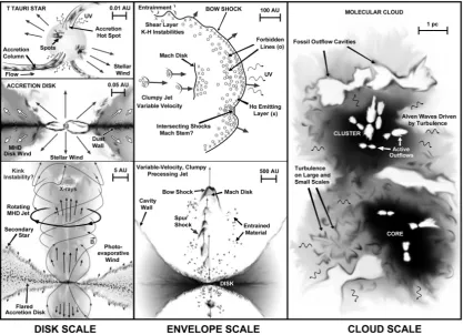
1.5 Outflows from YSOs at multiple scales . . . 16

1.6 Outflows in the HH 111 system . . . 18

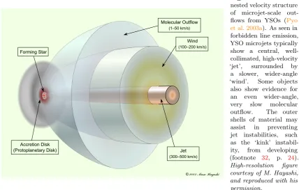
1.7 Nested structure of YSO microjets . . . 20

1.8 Rigid-wire analogy for MHD disc winds . . . 23

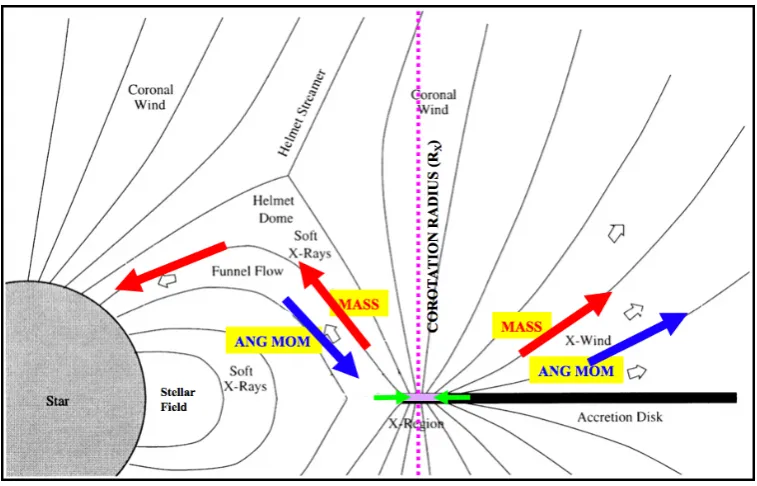
1.9 Schematic of the X-wind mechanism . . . 26

1.10 Spectral energy distribution of DG Tau . . . 29

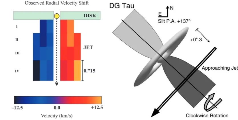
1.11 Investigations of rotation in the DG Tau outflows . . . 37

1.12 Herbig-Haro objects near DG Tau . . . 38

1.13 Integral-field unit designs . . . 40

2.1 Stellar spectrum of DG Tau, 2005 epoch . . . 52

2.2 Channel maps of the DG Tau outflow, 2005 epoch . . . 55

2.3 DG Tau approaching outflow, 2005 epoch . . . 56

2.4 DG Tau receding outflow, 2005 epoch . . . 59

2.5 Multicomponent Gaussian fits to approaching outflow emission . . . 60

2.6 Approaching outflow multicomponent line fits, 2005 epoch . . . 62

2.8 [Fe II] line ratios and electron density for approaching DG Tau outflows . . 64

2.9 Comparison of electron density measurements of the DG Tau jet . . . 65

2.10 Knots in the DG Tau microjet, 2005–2009 . . . 68

2.11 Knot evolution of the DG Tau microjet, 1997–2010 . . . 69

2.12 Launch radii estimates for innermost jet streamlines . . . 75

2.13 DG Tau approaching jet parameters, 2005 epoch . . . 77

2.14 DG Tau approaching jet mass flux, 2005 epoch . . . 78

2.15 Position-velocity diagram of approaching DG Tau outflow . . . 79

2.16 Velocity differences across the DG Tau jet ridgeline . . . 82

2.17 Cross-jet position-velocity diagrams . . . 83

2.18 Comparison of H2 and [Fe II] emission from DG Tau approaching outflow . 87 2.19 Position-velocity diagram of H2 and [Fe II] emission from approaching DG Tau outflow . . . 88

3.1 Schematic of mixing layer model . . . 99

3.2 Mixing layer boundary positions . . . 102

3.3 Mixing layer density, transverse velocity and turbulent stress profiles . . . . 103

3.4 Mixing layer entrainment velocity and mass gain . . . 104

3.5 Contribution to rate-of-change of mixing layer mass flux . . . 105

3.6 Growth rates of the approaching DG Tau outflow components . . . 110

3.7 Estimates of the DG Tau mixing layer [Fe II] 1.644 µm luminosity . . . 113

3.8 Theoretical estimates for DG Tau mixing layer parameters . . . 115

4.1 Channel maps of emission from the receding DG Tau outflow, 2005 epoch . 128 4.2 Single-component Gaussian fit to receding outflow emission, 2005 epoch . . 130

4.3 [Fe II] line ratios and electron density for receding DG Tau outflow . . . 131

4.4 Channel maps of emission from the receding DG Tau outflow, 2005–2009. . 132

4.5 The DG Tau receding bubble, 2005–2009. . . 133

4.6 Kinetic models of bubbles with expanding internal velocity fields . . . 135

4.7 Comparison of simulated IFS data of bubbles to observations . . . 137

4.8 H2 1-0 S(1) and [Fe II] emission from the DG Tau bubble . . . 141

4.9 Estimated bubble heights . . . 146

List of Tables

1.1 Properties of molecular clouds, clumps and cores . . . 4

1.2 Specific angular momentum through the star formation process . . . 13

1.3 Basic parameters of the DG Tau system . . . 27

1.4 Stellar and spectral parameters of the DG Tau system [Part I] . . . 28

1.4 Stellar and spectral parameters of the DG Tau system [Part II] . . . 29

1.5 Estimated disc accretion rates in DG Tau . . . 31

1.6 K-band CO bandhead emission/absorption in the spectrum of DG Tau . . 33

1.7 Estimates of the mass-loss rate in DG Tau approaching outflow [Part I] . . 35

1.7 Estimates of the mass-loss rate in DG Tau approaching outflow [Part II] . . 36

1.8 Available gratings for NIFS . . . 40

2.1 NIFS observations of DG Tau, 2005–2009 . . . 51

2.2 Knot positions in the approaching DG Tau jet, 2005 epoch . . . 57

2.3 Knot positions in the approaching DG Tau jet, 2005–2009 . . . 67

3.1 MAPPINGS IV shock model initial parameters . . . 107

3.2 Post-shock conditions and emission from MAPPINGS IV models . . . 109

Glossary and Acronyms

2MASS Two Micron All-Sky Survey AGN active galactic nuclei

ALMA Atacama Large Millimeter/Sub-millimeter Array

ALTAIR ALTtitude conjugate Adaptive optics for the InfraRed (Gemini North

AO system) AO adaptive optics

BE99 Bacciotti & Eisl¨offel(1999) method for determining gas parameters from

optical line ratios (see footnote 40, p.34) CTTS classical T Tauri star (§1.1.2.1)

FEL forbidden emission line FHSC first hydrostatic stellar core FUV far-ultraviolet

FWHM full width at half-maximum GMC giant molecular cloud

GMT Giant Magellan Telescope

GMTIFS Giant Magellan Telescope Integral Field Spectrograph

HH Herbig-Haro, e.g. Herbig-Haro object HST Hubble Space Telescope

HVC/I high-velocity component/interval

IFS integral-field spectrograph (IFU plus spectrograph; §1.4) IFU integral-field unit (§1.4)

IR infrared

IUE International Ultraviolet Explorer

IVC intermediate-velocity component

MHD magnetohydrodynamic(s)

MRI magnetorotational instability (§1.1.3) MVC/I medium-velocity component/interval

NICMOS Near Infrared Camera and Multi-Object Spectrometer (HST instrument) NIFS Near-infrared Integral Field Spectrograph (Gemini North instrument;

§1.4)

NIR near-infrared

PACS Photoconductor Array Camera and Spectrometer (Herschel instrument) PBRS PACS bright red source (Fig. 1.2)

PSF point spread function

SED spectral energy distribution (§1.1.2.2)

STIS Space Telescope Imaging Spectrograph (HST instrument)

TTS T Tauri star (§1.1.2.1) UV ultraviolet

VeLLO very low-luminosity object (Fig. 1.2)

WFPC2 Wide Field and Planetary Camera 2 (HST instrument) WTTS weak-lined T Tauri star (§1.1.2.1)

YSO young stellar object ZAMS zero-age main sequence

CHAPTER 1

Introduction

But if the matter were evenly disposed throughout an infinite space, it could never convene into one mass; but some of it would convene into one mass and some into another, so as to make an infinite number of great masses, scattered great distances from one to another throughout all of that infinite space. And thus might the sun and fixed stars be formed. . .

– Isaac Newton1

Collimated outflows are ubiquitous components of accreting astrophysical objects across a wide range of masses and energies. The masses of outflow-driving systems range from

supermassive black holes in active galactic nuclei to sub-solar mass protostellar cores and white dwarfs. The wide range of objects that are capable of launching jets, winds and

related outflow types2 _{suggest that some universal underlying mechanism is at work. This}

mechanism is believed to be tied to the gravitational accretion of material and the need for

an efficient method of removing angular momentum (Smith 2012). Although it is generally accepted that these outflows are launched via magnetohydrodynamic processes (e.g.Livio 1999), the exact details of this mechanism or mechanisms remain elusive.

Outflows are thought to play a particularly important role in the process of star formation. They are the means by which young stars clear their environment, allowing them to become

optically revealed to observers. The outflows are also used as a signature to ascertain the

1_{Letter to Richard Bentley (Jeans 1929;Larson 2003).}

2_{Throughout this thesis we use the following nomenclature. Outflowsencompass all types of collimated}

presence of forming stars before they are revealed. Outflows may modify the structure of

protostellar discs (Combet & Ferreira 2008), affect the penetration of ionizing particles and stellar radiation into the disc (Desch et al. 2004;Cleeves et al. 2013), lead to the formation of

a disc corona (Fleming & Stone 2003), lift and process dust particles (Safier 1993;Salmeron & Ireland 2012), accelerate disc dispersal (Suzuki & Inutsuka 2009), and limit the extent of

infalling gas via feedback (Arce & Sargent 2004). Finally, and perhaps most importantly, outflows are thought to aid in overcoming the angular momentum problem (§1.1.3) which would otherwise impede the ability of a protostar to accrete matter. Therefore, a thorough

understanding of the structure of outflows, and how they are launched, is vital to unravelling the mystery of how stars like the Sun, and potentially solar systems like our own, form.

Protostellar outflows have been studied extensively in the literature (§1.2) using spectro-scopic and imaging techniques. However, spectroimaging techniques (e.g. §1.4) remain relatively underutilized. The combination of structural and kinematic information that may be obtained using an integral-field spectrograph allows for a highly-detailed analysis of the structure, kinematics and, with the inclusion of multi-epoch data, variability in

protostellar outflows. The use of adaptive-optics systems allows the outflows to be resolved within tens to hundreds of AU of the driving source.

In this thesis, we present the deepest spectroimaging observations to date of the protostellar outflows associated with the actively-accreting young star DG Tauri. These data (§2) allow us to rigourously separate the emission from blended outflow components for the first time, and probe the parameters and structure of each in exquisite detail. We leverage these data to investigate critical questions in the field of protostellar outflows, such as the presence

of rotation, the launch radii of the outflow components, the interactions between outflow components and ambient media, the generation of periodic and time-variable structures,

and the self-similarity of the outflow components. The data motivate us to develop original analytical models of the processes by which the outflow components may interact with each

other (§3), and with the ambient medium surrounding the protostar (§4). We demonstrate that the intermediate-velocity component of the approaching outflow is consistent with the formation of a turbulent mixing layer, and that the receding outflow ‘bubble’ structure is a

sign of jet-ambient medium interaction. These models represent fundamental progress in the field of protostellar outflows, and have wide implications in the study of outflows from

other young stellar objects.

In the balance of this chapter, we provide an overview of the star formation process, and

the basic properties of low-mass protostars. We then discuss the role that outflows may play in star formation, as well as some key observations of these beautiful systems. We provide a summary of our object of interest, DG Tauri, as well as the instrument we used

1.1.

Star Formation

Star formation is one of the most important processes in astrophysics. Stars are the

fundamental units, indeed, ‘atoms’ of the Universe. They determine the structure and evolution of galaxies, play a dominant role in the generation of almost all observed luminosity, and possibly led to the reionization of the Universe. All elements beyond hydrogen and

helium are formed in stars, and the process of star formation is inextricably linked to the formation of planetary systems (McKee & Ostriker 2007). Therefore, determining the exact

nature of star formation is of central importance (Shu et al. 1987). Whilst the general picture of star formation is thought to be fairly well-understood (§1.1.1), there remain several outstanding problems (e.g.§1.1.3).

1.1.1. Overview of the Star Formation Process

The overarching picture of the process of star formation as the accumulation and collapse of overdensities in the interstellar medium has been around since at least the times of Newton

(Larson 2003). However, further significant advances in the theory of star formation were not made until the middle of the 20th _{century, when it was realized by Ambartsumian} (1947) that star formation was ongoing nearby in the Milky Way, and that contemporary

telescope technology allowed for the detailed analysis of these objects. Subsequently, millimetre-wave CO observations in the 1970s provided direct detection of the seed material

for star formation in clouds, clumps and cores (e.g. Lada 1987). The core concepts of the star formation process were reasonably well-understood by the 1980s, and are encapsulated

in the review ofShu et al. (1987). However, many details of the star formation process remain unclear, and the search for a complete model of star formation remains one of the most fundamental outstanding questions of astrophysics.

The remainder of §1.1.1 provides a brief outline of the basic concepts of star formation. It is not intended to address all the outstanding questions the field; the reader is invited to

consult the reviews ofLada(1987),Shu et al.(1987),Larson(2003) andMcKee & Ostriker (2007), as well as the recent textbook ofBodenheimer (2011), for a more comprehensive

account.

1.1.1.1. Molecular Clouds, Clumps and Cores

Massive (_∼107 _M

) bound structures condense from the diffuse interstellar medium in

galactic spiral arms due to large-scale gravitational instabilities (Larson 2003;

Ballesteros-Paredes et al. 2007). These structures inherit a large amount of turbulence from the diffuse ISM which, along with self-gravity, causes them to fragment into giant molecular

Table 1.1 Properties of molecular clouds, clumps and cores. Adapted fromBodenheimer(2011).

Giant molecular cloud

Molecular cloud

Molecular clump

Cloud core

Mean radiusa _{(pc) 20 5 2 0.08 (∼10}4 _AU)

Number density,a _n

H2 (cm

−3_{) 10}2 _3×102 ₁₀3 ₁₀5

Massa _(M

) 105 104 103 101

Linewidth (km s−1_{) 7 4 2 0.3}

Temperature (K) 15 10 10 10

a_{Values quoted are indicative only; a wide range of masses and sizes are possible.}

clouds may be formed by ram pressure from supersonic flows, which are potentially driven by an ensemble of supernova explosions, superbubbles and expanding HII regions

(Ballesteros-Paredes et al. 2007).

Molecular clouds are strongly structured, being dominated by density enhancements referred

to as clumps that are the progenitors of star clusters (McKee & Ostriker 2007). Two basic processes may be involved in the fragmentation of molecular clouds. Fragmentation may result from small inhomogeneities in the original molecular cloud distribution that

are amplified by self-gravity. Alternatively, the relationship of increasing linewidth, and inferred velocity dispersion, to increasing cloud size (Table1.1) suggests the presence of a hierarchy of supersonic turbulence within the clouds. Such supersonic turbulence would compress the gas in shocks, creating a hierarchy of compressed clumps. Both processes

almost certainly play a role in fragmenting clouds down to the clump regime (Larson 2003). The same processes lead the clumps to further fragment into molecular cores (§1.1.1.2), which are the progenitors of single- or multiple-star systems. Typical bulk properties of

molecular clouds, clumps and cores are listed in Table 1.1.3

1.1.1.2. Protostellar Collapse

The evolutionary steps by which a region of a molecular clump collapses to form an

optically-revealed, low-to-intermediate mass young stellar object (YSO) was first summarized in the review ofShu et al.(1987), and is shown in Fig.1.1. Our understanding of this overarching process has not changed significantly since then, although many of the underlying processes

are still actively investigated.

Two main models to explain molecular cloud core collapse exist (Fig.1.1a). The first, based on analyses of the stability of molecular clouds and the fragmentation process, suggests that an unstable or marginally stable clump of gas, in which gravity overcomes pressure,

3_{It is important to note that while this fragmentation process is expressed in terms of discrete stages, it}

1.1 Star Formation 5 by which angular momentum is transported outward as material is accreted is still unclear. The deeply embedded protostar undergoes slow hydrostatic compression and internal energy transport is largely radiative. The star and its encircling nebular disk continue to accrete gas and dust from the infalling envelope and the luminosity of this system is dominated by accretion processes. Radiation from matter as it falls through accretion shocks onto the protostar and disk is thought to produce the excess emission features in the spectral energy distribution that characterise the protostellar phase. Growth in the radius of the protostar ceases when matter outside the accretion shock becomes transparent and radiation escapes freely from the star, halting the heating and expansion of the outer layers.

Stage 3: Bipolar outflow and disk accretion (Figure 1.1c)

Deuterium ignites in the core of the protostar when compression under the growing mass generates the required temperature, and convective energy transport soon dominates the

1987ARA&A..25...23S

Figure 1.1 The four stages of star formation, illustrated by Shu in his detailed 1987 review paper. (a) The magnetic and turbulent support in molecular clouds is depleted by ambipolar di↵usion, initiating the contraction of gas into higher-density cloud cores. (b) The molecular cloud core collapses from the inside-out, when the small central region reaches unstable densities, and an accreting protostar and disk system forms inside the envelope of the gradually infalling cloud. (c) Material begins to accrete primarily onto the circumstellar disk, rather than directly onto the star, allowing stellar winds to be channelled into bipolar jets. (d) The new protostar is optically visible in the T Tauri stage. There is still significant encircling material in the disk, and accretion and outflowing jets continue to be active during early pre-main sequence evolution.

Figure 1.1 The evolution of forming stars (Shu et al. 1987). (a) Regions of molecular clouds become unstable, and begin to collapse to form protostellar cores. (b) The core develops a central density peak, which forms a protostar surrounded by a circumstellar disc. Material from the core continues to fall on to the circumstellar disc. (c) Disc accretion begins to drive bipolar outflows, which start to clear out the remnant protostellar envelope. (d) Infall from the envelope to the disc ceases, and the subsequent disc accretion then stops. The related outflows also terminate, leading to a pre-main-sequence protostar surrounding by a passive protostellar disc. Reproduced with the permission of Annual Reviews.

initiates a rapid runaway collapse (fast-collapse model; Hayashi 1966;Ward-Thompson 2002). The unstable clumps are formed as the result of supersonic turbulence within the molecular cloud complex (Larson 1981;Ballesteros-Paredes et al. 2007;Bodenheimer

2011). The second model states that cloud cores are initially magnetically supported, and condense slowly as magnetic support is leaked away via ambipolar diffusion (slow-collapse

model;Shu 1977;Shu et al. 1987,2004;Bodenheimer 2011; Li et al. 2014). In a magnetized plasma, the magnetic field is coupled to the charged particles, which are in turn coupled to the neutral particles via collisions. For weakly ionized plasmas, the neutrals and charged

particles become decoupled as the collision rate becomes negligible, removing the support of the magnetic field from the neutrals and leaving them subject to gravitational collapse

(Mestel & Spitzer 1956). Both of these models represent unphysical extremes; more realistic models are expected to be intermediate to the above scenarios (Larson 2003).

collapse (Shu 1977;Shu et al. 1987;Larson 2003). In the slow-collapse model of Shu et al.

(1987), the surface at which gas begins to fall quickly inwards propagates outwards through the quasi-static core at the sound speed (Shu 1977). In the fast-collapse scenario (Hayashi

1966), the mass infall rate on to the nascent protostar is much higher, and material falls in at a few times the sound speed from an already-infalling core (e.g.Larson 1969). Again,

reality is likely to exist somewhere between these two extremes (Larson 2003). Regardless, the net result of this collapse is the formation of a very low-mass (. 10−2 _M

;Larson

2003) protostar in the centre of the cloud core (Figure 1.1b; McKee & Ostriker 2007).4

The remainder of the cloud core continues to collapse inwards.

Most star-forming cores are rotating (Goodman et al. 1993), as would be expected for

turbulent molecular clouds (Burkert & Bodenheimer 2000). Material is present with sufficient angular momentum to prevent it from falling directly onto the protostar, instead

forming a circumstellar accretion disc (Figure 1.1b;Larson 2003; McKee & Ostriker 2007). As the collapse proceeds, material will fall preferentially onto the disc as opposed to the star (Shu et al. 1987). This occurs because material at greater distances from the star,

with greater angular momentum, begins to undergo infall (Terebey et al. 1984;Hartmann 1998). Subsequently, material accretes through the disc onto the central star, although the

method by which the material sheds excess angular momentum remains unclear (§1.1.3).5

Throughout the initial accretion phase, the central star remains heavily obscured by the

cloud core, making direct observation of this process difficult. Indeed, the star is typically not optically revealed until the majority of mass accretion has already occurred (Larson 2003).6 _{During this phase, the main contribution to the luminosity of the system comes}

from accretion shocks on the central star and circumstellar disc, which gives rise to the

4_{This actually takes the form of a two-phase collapse process. The first collapse ceases when the gas}

in the central density peak becomes hot enough to support the central hydrostatic core against further collapse. Once this gas reaches temperatures capable of dissociating molecular hydrogen, the value of the adiabatic index in the core drops below the critical value of 4/3 required for stability (Larson 2003), leading to the second collapse and the formation of the protostar (McKee & Ostriker 2007). The majority of the first hydrostatic core has collapsed into the second core within∼10 years (Larson 2003).

5_{It should be noted that, in the last decade, it has been realized that the strong magnetic fields of}

protostellar cores may effectively brake the core rotation as it collapses. Thismagnetic braking occurs when the magnetic field lines threading the disc are twisted by the disc’s rotational motion, loading up the tension in the field lines. Alfv´en waves then transfer angular momentum from the disc to the external medium, not unlike waves travelling along a taut, plucked rubber band (K¨onigl & Salmeron 2011). This would solve the angular momentum problem, but prevent the formation of Keplerian rotation discs. Given the fact that such discs are ubiquitous throughout star formation, and are even starting to be detected in Class 0 objects (e.g.Tobin et al. 2012,2013;Murillo et al. 2013), this is an outstanding issue, referred to as the ‘magnetic braking catastrophe’. Although ambipolar diffusion and the Hall effect have a significant effect on the collapse process (Li et al. 2011;Braiding & Wardle 2012a,b), it is currently thought that turbulence and Ohmic dissipation are the key physical mechanisms for limiting the effectiveness of magnetic braking, and allowing the formation of rotationally-supported discs around forming stars (Li et al. 2014, and references therein). Recent simulations using multiple levels of spatial refinement suggest a two-phase core collapse process; an initial efficient shedding of angular momentum until approximately half the initial protostellar mass is accreted, followed by the formation of a rotationally-supported protoplanetary disc at later stages (Nordlund et al. 2014).

6_{The advent of the Atacama Large Millimeter/Sub-millimeter Array (ALMA) is expected to begin to}

As the protostar continues to accrete matter, deuterium ignition will occur in the core when the required temperature is reached (approximately 1_×106 _{K; Shu et al. 1987),} approximately when the protostar reaches a mass ∼0.2 M. This is a significant source

of heat, which greatly slows protostellar contraction as accretion continues (Larson 2003).

Furthermore, differential rotation, coupled with the convection driven by deuterium burning, can produce dynamo action and generate strong magnetic activity. The energy released may power the intense stellar surface activity observed in YSOs (Shu et al. 1987). As material

preferentially falls on the circumstellar disc as opposed to the star, the ram pressure of the direct infall weakens above the rotational poles (Shu et al. 1987). This allows the outflows

from the central star/inner disc to break clear of the circumstellar envelope and begin clearing it (Fig.1.1(c)). In the original paradigm ofShu et al. (1987), these outflows were thought to be stellar winds, but it has been realized since that they are far more likely to be magnetohydrodynamic winds launched from the disc surface (§1.2;Li et al. 2014). As the envelope material is swept away, the star becomes optically revealed for the first

time, and is observed as a T Tauri star (TTS) or Herbig Ae/Be star, depending on the protostar mass and spectral properties (§1.1.2). These stars emerge on the ‘birthline’ of the Hertzsprung-Russell diagram, and descend steep Hayashi tracks towards the zero-age main sequence (ZAMS;Stahler 1983). After the envelope around the protostar is dispersed,

and full hydrostatic equilibrium is reached, the protostar contracts on a Kelvin-Helmholtz timescale until hydrogen fusion begins, and the star enters the main sequence.

1.1.2. The Classification of Protostars

1.1.2.1. By Mass and Spectral Features

The primary discriminant for the classification of YSOs is mass. High-mass YSOs, with masses&8–10 M, make up the ‘massive YSOs’. These objects may form via a scaled-up

version of the process described in §1.1.1.2, or via the so-called ‘competitive accretion’ process in dense clusters (Tan et al. 2014;Krumholz 2014).7 _{The low-mass YSOs are split}

into two further classes; the low-mass T Tauri stars, and the intermediate-mass Herbig Ae/Be stars. Conceptually, T Tauri and Herbig Ae/Be stars are differentiated by mass, with the mass cut between the two classes at _∼2–3 M.8 However, the formal separation

7_{A detailed discussion of the process of massive star formation is beyond the scope of this thesis. The}

interested reader is directed to the reviews ofHoare et al.(2007),Tan et al.(2014) andKrumholz(2014) for details.

8_{The exact mass break between the two classes varies between authors. Appenzeller & Mundt(1989)}

place the cutoff at 3 M,Feigelson & Montmerle(1999) adopt a value of 2 M, and bothHillenbrand et al.

(1992) andAlecian et al.(2007) allow Herbig Ae/Be stars to have masses as low as 1.5 M. Therefore, there

is made via spectroscopic properties. The balance of this section focuses on the T Tauri

class of protostars.

T Tauri stars (TTS) were first identified from the prototype object T Tauri by Joy (1945),

who proposed a set of relatively tightly-defined spectral and light-variation characteristics for the class. Herbig(1958), whilst noting their near-universal variability, determined that the classification of TTS should be made on spectroscopic properties alone, and provided a

broadened, but highly-prescriptive definition (Herbig 1962). Bastian et al.(1983) realized that this definition was unnecessarily dependent on transient spectral features, and also

excluded some TTS which were lacking one or two typical attributes of the class. Therefore, they determined a simplified definition of a T Tauri star:

Stellar objects associated with a region of obscuration; in their spectrum they

exhibit Balmer lines of hydrogen and the Ca II H and K lines in emission, the equivalent width of Hα being at least 5˚A. There is no supergiant or early-type (earlier than late F) photospheric absorption spectrum.9

This definition, whilst still frequently used, is not complete; e.g. the Balmer emission lines

of TTS are known to vary significantly with time (Appenzeller & Mundt 1989). Presently, the term TTS is synonymous with low-mass pre-main-sequence stars, irrespective of

their emission characteristics (Hartmann 1998); these objects are identified by a range of techniques such as objective prism surveys, X-ray surveys, proper motion, photometry and variability studies, and their classification is confirmed spectroscopically (Brice˜no

et al. 2007). Identification of young stars by comparison to theoretical stellar evolution models using colour-magnitude diagrams is the most common approach (e.g. Bouvier &

Appenzeller 1992;Hughes et al. 1994;Luhman et al. 2003).

TTS typically have late spectral classes (late F to M, Petrov 2003), with strong excess IR and UV emission. In some cases, the IR excess is so pronounced that the peak of the

spectral energy distribution is shifted into the far-infrared (§1.1.2.2;Rydgren et al. 1984; Bertout 1989), and the presence of hot dust, at an inferred temperature of hundreds of K,

must be invoked. The UV/blue excess is radiation released by free-free and free-bound transitions in a hot hydrogen plasma, most likely formed in the accretion process (Petrov 2003).

More specifically, the spectrum of a TTS may be broken into four components — a stellar continuum, a stellar absorption line spectrum, a superimposed non-photospheric continuum,

and an emission-line spectrum. The stellar absorption line spectrum is similar to that of a late-type (K to M) dwarf, with strongly enhanced Li I 6708 ˚A absorption (Appenzeller & Mundt 1989), which is indicative of the youth of the star (Skumanich 1972;Bertout 1989;

9_{TheBastian et al.(1983) definition of a Herbig Ae/Be star is similar, but the stellar object is earlier}

‘veiled’ by the non-photospheric continuum (e.g.Greene & Lada 1996;Doppmann et al. 2005).10 _{Approximately two-thirds of TTS show double-peaked Balmer lines (Appenzeller}

& Mundt 1989), which provide evidence for complex and time-varying gaseous flows in the envelopes of these stars (Bertout 1989). The emission-line profiles are broadened, and the

forbidden lines enhanced (§1.2).

TTS are further classified by their spectra intoclassical (CTTS) andweak-lined (WTTS)11

T Tauri stars. CTTS are those objects that broadly conform to the characteristics described

above. As the name suggests, WTTS exhibit weaker line emission, particularly in the Balmer and forbidden lines (Appenzeller & Mundt 1989;Bertout 1989;Cieza et al. 2007).

They also show little to no UV and IR excess in their spectral energy distributions. The physical reasons behind these differences are elaborated in §1.1.2.2.

1.1.2.2. By Spectral Energy Distribution

Starting in the 1980s, a classification scheme for YSOs was developed based upon the spectral energy distribution (SED, the product of wavelength, λ, and intensity at that wavelength, Fλ, as a function of λ) of the objects.12 This classification scheme was based

both on the observed SEDs and on theoretical modelling, and was hence perceived to be more meaningful as a measure of the evolutionary state of the YSO.Lada(1987) was the

first to introduce a three-tier class system, and Adams et al. (1987) proposed a similar classification scheme. The hallmark of both systems is the classification of stellar objects

using the slope of their SED in log-log space,

α≡ d log(λFλ)

d logλ , (1.1)

over the wavelength range 2.2 µm to 10–25 µm (e.g. McKee & Ostriker 2007). Andr´e

et al. (1993) added an additional class, Class 0, based on the sub-millimetre luminosity of deeply-embedded objects. Examples of the SEDs used to classify protostars are shown

in Figs 1.2 and 1.3. The resulting classification leads to an evolutionary track, where protostars begin as Class 0 objects, and move through Classes I, II and III as they evolve

(Andr´e et al. 2000). This system may be summarized thus (McKee & Ostriker 2007):13

10_{This veiling was first noted by Joy (1945). The term is now understood to refer to two distinct}

phenomena that cannot be easily differentiated in observations: (a) selective filling in of spectral lines, and (b) overlying continuum emission (Bertout 1989). Veiling in classical TTS can be so strong that it can only be explained by the presence of a non-photospheric continuum, which may exceed the photospheric continuum by a factor of several (Petrov 2003).

11_{These objects are occasionally referred to asnaked T Tauri stars (e.g.Walter et al. 1988).} 12_{SEDs may also be expressed in terms of frequency,νvs.F}

νν(Adams et al. 1990). λFλandνFνare units of energy, not energy density; SEDs are determined in these units to remove any dependence on the size of the wavelength/frequency bins used.

13_{There are variations on this classification scheme. For example,Allen et al.(2007),Williams & Cieza}

Fig. 1.—

Laun-hardt et al., 2013), a candidate first hydrostatic core (Pineda et al.,

2011), a very low-luminosity object (Dunham et al., 2008;Green

et al., 2013b), a PACS bright red source (Stutz et al., 2013), a

Class 0 protostar (Stutz et al., 2008;Launhardt et al., 2013;Green

et al., 2013b), a Class I protostar (Green et al., 2013b), a Flat-SED

source (Fischer et al., 2010), and an outbursting Class I protostar

(Fischer et al., 2012). The+and×symbols indicate photometry,

triangles denote upper limits, and gray lines show spectra.

core and disk material has dissipated.

Chen et al.

(1995)

proposed the following Class boundaries in

T

: 70 K

(Class 0/I), 650 K (Class I/II), and 2800 K (Class II/III).

With the sensitivity of

Spitzer

, Class 0 protostars are

rou-tinely detected in the infrared, and Class I sources by

α

are

both Class 0 and I sources by

T

(

Enoch et al.

, 2009).

Additionally, sources with flat

α

have

T

consistent with

1000 100 10

Bolometric Temperature (K)

10-5 10-4 10-3 10-2 10-1 100

Submillimeter / Bolometric Luminosity

Tbol Class 0

Tbol Class I

Tbol Class II

Lsmm/Lbol Class 0

Lsmm/Lbol Class I

c2d+GB HOPS PBRS

Fig. 2.—

in the c2d, GB, and HOPS surveys. The PBRS (§4.2.3) are the 18 Orion protostars that have the reddest 70 to 24 µm colors, 11 of which were discovered with Herschel. The dashed lines show the Class boundaries inTbol fromChen et al.(1995) and in

Lsmm/Lbol fromAndre et al.(1993). Protostars generally evolve

from the upper right to the lower left, although the evolution may not be monotonic if accretion is episodic.

Class I or Class II, extending roughly from 350 to 950 K,

and sources with Class II and III

α

have

T

consistent with

Class II, implying that

T

is a poor discriminator between

α

-based Classes II and III (

Evans et al.

, 2009).

T

may increase by hundreds of K, crossing at least

one Class boundary, as the inclination ranges from edge-on

to pole-on (

Jorgensen et al.

, 2009;

Launhardt et al.

, 2013;

Fischer et al.

, 2013). Thus, many Class 0 sources by

T

may in fact be Stage I sources, and vice versa. Far-infrared

and submillimeter diagnostics have a superior ability to

re-duce the influence of foreground reddening and inclination

on the inferred protostellar properties. At such wavelengths

foreground extinction is sharply reduced and observations

probe the colder, outer parts of the envelope that are less

optically thick and thus where geometry is less important.

Flux ratios at

λ

_≥

70

µ

m respond primarily to envelope

density, pointing to a means of disentangling these effects

and developing more robust estimates of evolutionary stage

(

Ali et al.

, 2010;

Stutz et al.

, 2013). Along these lines,

sev-eral authors have recently argued that

L

/

L

is a better

tracer of underlying physical Stage than

T

(

Young and

Evans

, 2005;

Dunham et al.

, 2010a;

Launhardt et al.

, 2013).

Recent efforts have vastly expanded the available 350

µ

m data for protostars via, e.g., the

Herschel

Gould Belt

survey (see accompanying chapter by

Andr´e et al.

),

sev-eral

Herschel

key programs (e.g.,

Launhardt et al.

, 2013;

Green et al.

, 2013b), and ground-based observations (e.g.,

4

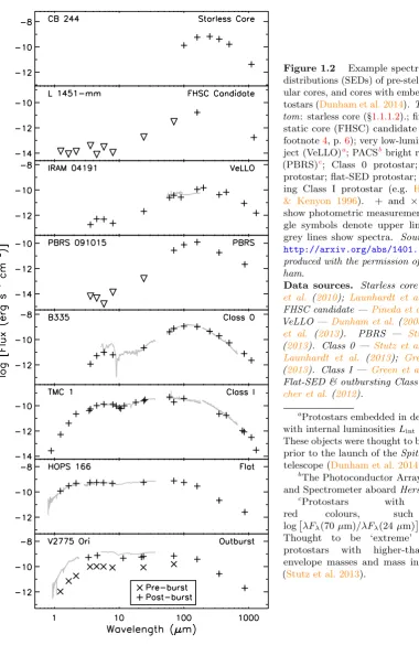
Figure 1.2 Example spectral energy distributions (SEDs) of pre-stellar molec-ular cores, and cores with embedded pro-tostars (Dunham et al. 2014). Top to bot-tom: starless core (§1.1.1.2).; first hydro-static core (FHSC) candidate (§1.1.1.2; footnote4, p.6); very low-luminosity ob-ject (VeLLO)a_{; PACS}b_{bright red source}

(PBRS)c_{; Class 0 protostar; Class I}

protostar; flat-SED protostar; outburst-ing Class I protostar (e.g. Hartmann & Kenyon 1996). + and _× symbols show photometric measurements, trian-gle symbols denote upper limits, and grey lines show spectra. Sourced from

http://arxiv.org/abs/1401.1809. Re-produced with the permission of M.

Dun-ham.

Data sources. Starless core — Stutz et al. (2010); Launhardt et al. (2013).

FHSC candidate —Pineda et al.(2011).

VeLLO —Dunham et al. (2008);Green

et al. (2013). PBRS — Stutz et al.

(2013). Class 0 —Stutz et al. (2008);

Launhardt et al. (2013); Green et al.

(2013). Class I —Green et al.(2013).

Flat-SED & outbursting Class I —

Fis-cher et al.(2012).

a_{Protostars embedded in dense cores}

with internal luminositiesLint≤0.1 L.

These objects were thought to be starless prior to the launch of theSpitzer space telescope (Dunham et al. 2014).

b_{The Photoconductor Array Camera}

and Spectrometer aboardHerschel.

c_{Protostars with very}

red colours, such that

log

λFλ(70µm)/λFλ(24µm)

> 1.65.

Figure 1.3 Typical spectral energy distribu-tions (SEDs) for Class I, II and III protostars (Lada 1987). Class I:SED broader than a blackbody, with positive spectral indices red-ward of 2µm. Class II:SED broader than a blackbody, with flat or negative spectral in-dices redward of 2µm. Class III: Well-fit by a reddened blackbody function. The con-tinued decrease of the infrared excess in the SED from Class I to Class III indicates the accretion and dissipation of the protostellar envelope (Class I to Class II) and circumstellar disc (Class II to Class III;Dunham et al. 2014).

Reproduced with the permission of C. Lada.

1987IAUS..115....1L

Class 0: Sources with a central protostar that is very faint in the optical/near-IR14_,

and a significant sub-millimetre luminosity15_{, L}

smm, such that Lsmm/Lbol >0.5%, where Lbol is the bolometric luminosity. Their SEDs resemble a single-temperature blackbody withT _∼15–30 K. Class 0 sources are condensations in molecular cores

that appear to be associated with formed, hydrostatic YSOs (Andr´e et al. 1993,2000). These objects are just beginning the process of star formation, with the central object

starting with significantly less mass than the final stellar mass (§1.1.1.2; Andr´e et al. 2000; White et al. 2007). A significant fraction of the stellar mass is accreted during

between Classes II and III is atα=−1.6, Class I hasα≥0.3, and a new class, termed ‘flat-SED’ sources, is inserted between Classes I and II for sources with₋0.3_≤α <0.3. Other reviews choose not to incorporate flat-SED sources in their classification system (McKee & Ostriker 2007), although some do note them as an interesting sub-class of objects (e.g.White et al. 2007). Flat-SED sources are discussed further at the end of§1.1.2.2.

14_{That is, effectively undetectable in these regimes using 1990s-era technology (McKee & Ostriker 2007).} 15_L

this stage (McKee & Ostriker 2007). These objects roughly correspond to Fig. 1.1(a).

Class I: Sources withα > 0. In this phase, material from the envelope is infalling on to the circumstellar disc (Dunham et al. 2014). The central protostar is relatively evolved, having accreted most of its mass during its Class 0 phase (McKee & Ostriker

2007;White et al. 2007). This stage corresponds to Fig. 1.1(b) and (c).

Class II: Sources with −1.5< α <0. These are pre-main sequence stars with significant circumstellar discs (classical TTS;§1.1.2.1). Both circumstellar discs and large-scale outflows are easily observable at this stage, whilst some accretion (.10−8 _M

yr−1)

is ongoing (Hartigan et al. 1995;McKee & Ostriker 2007). This stage corresponds to somewhere between Figs1.1(c) and (d).

Class III: Sources with α <₋1.5. This stage is reached when accretion onto the central star, and the resulting outflow activity, has largely ceased (weak-lined TTS;McKee

& Ostriker 2007). This results in the disappearance of the SED emission excesses and forbidden emission lines. Class III SEDs are well-fit with a reddened blackbody

function, indicative of a star close to the zero-age main sequence surrounded by a ‘passive’ protoplanetary disc which re-radiates stellar light (Petrov 2003). There may

also be a complete lack of circumstellar material (Dunham et al. 2014). This stage corresponds to Fig.1.1(d).

It should be noted that the above classification scheme is a binning of the continuous evolution of SED spectral index (Lada 1987), and by extension the continuous star formation

process. Indeed, some authors cite an additional evolutionary stage, the transitional Class I/Class II objects (also called the flat-SED objects, see footnote13, p. 11;Greene et al. 1994; Allen et al. 2007; Dunham et al. 2014). These objects have characteristics of Class II objects, such as well-collimated microjet-scale outflows (§1.2.1.3), but are more heavily obscured, or have higher mass accretion rates, or large remnant protostellar envelopes, like

Class I objects.

The linkage between the IR and UV excesses in YSO spectra is of particular importance.

It has been observed that YSOs with IR excesses almost invariably have strong optical/UV excess emission; conversely, all objects which display signs of active accretion also show

IR excesses associated with the presence of an accretion disk (Hartigan et al. 1995). This correlation reveals that the powering of excess emission, and the driving of jets and winds16_,

comes from the energy released in the accretion process (Cabrit 2007b). This motivates

the development of models which link the accretion process with the launch of collimated outflows (§1.2.2).

16_{Hartigan et al.(1995) found a strong correlation between mid-infrared excess emission and [O I] 6300 ˚A}

the process of star formation. There is a clear need for the loss of angular momentum throughout protostellar collapse and mass accretion. Adapted from Bodenheimer(2011).

Object Scale J/M (cm2 _s−1₎

Molecular clump 1 pc 1023

Cloud core 0.1 pc 1.5_×1021

Typical disc around 1 M protostar 100 AU 4.5×1020

T Tauri star (rotation) few R 5.0×1017

Sun (rotation) R 1015

Jupiter (orbit) 5.2 AUa ₁₀20

a_{Young & Freedman(2004)}

Much like the realization that different types of active galactic nuclei (AGN) represent

different viewing angles on to the same kind of object (Antonucci 1993;Urry & Padovani 1995), the geometry of a particular YSO, including inclination, aspherical geometry and foreground reddening effects, can confuse this classification system (McKee & Ostriker

2007;Dunham et al. 2014). For example, the simulations of protostellar collapse performed byMasunaga & Inutsuka (2000) showed that objects that would be assigned to Class I

conceptually based on their evolutionary state may have SEDs characteristic of Class 0 sources if the system is viewed ‘edge-on’ to the nascent circumstellar disc. White et al.

(2007) also point out that the properties of many Class I and Class II sources, such as effective temperature, photospheric luminosity and stellar mass, are similar, further suggesting that inclination effects may be confusing the classification system. There was

much discussion at the recent Protostars & Planets VI meeting on the need for a more robust and meaningful classification system. It is hoped sub-millimetre instruments such

as ALMA will be able to penetrate protostellar cores and reveal their true nature, allowing a classification system based on precise position on the star formation sequence to be

developed.

1.1.3. Disc Accretion and the Angular Momentum Problem

The mechanism of accretion on to the central protostar remains poorly understood. This is

due in large part to the accretion process being a complex interplay of magnetohydrodynam-ics, radiative transfer, chemistry, and possibly solid-state physics (McKee & Ostriker 2007). One clear constraint is that throughout the process of star formation, there is a continued

need to remove angular momentum from the collapsing protostellar system. Observations show that at each stage of the star formation process, from core to ZAMS, the system must

Fig. 3.The magnetorotational instability. Magnetic fields in a disk bind fluid el-ements precisely as though they were masses in orbit connected by a spring. The inner elementmiorbits faster than the outer elementmo, and the spring causes

a net transfer of angular momentum frommitomo. This transfer is unstable, as

described in the text. The inner mass continues to sink, whereas the outer mass rises farther outward. (Figure courtesy of H. Ji.)

separation of the displaced fluid elements, which is followed by the nonlinear mixing of gas parcels from different regions of the disk. The mixing seems to lead to something resembling a classical turbulent cascade, though the details of this process, with different viscous and resistive dissipation scales, remain to be fully understood.

Notice that angular momentum transport is not something that happens as a consequence of the nonlinear development of the MRI, it is the essence of the MRI even in its linear phase. The very act of transporting angular momentum from the inner to outer fluid elements via a magnetic couple is a spontaneously unstable process.

4.3 General Adiabatic Disturbances

IfΩis a function only of cylindrical radiusR, then for general magnetic field geometries, local incompressible WKB disturbances with space-time depen-dence

Figure 1.4 The magnetorotational instablil-ity (MRI, Balbus 2011). Disc magnetic fields bind fluid elements in the same fashion as springs may bind masses in orbit. As the in-ner element, mi, orbits the central mass, Mc, faster than the outer element, mo, the mag-netic field ‘spring’ causes a net transfer of an-gular momentum from mi to mo. This forces

mi to move inwards, and mo to move further out in an unstable, runaway process. Original figure courtesy H. Ji; sourced from Scholarpe-dia (http://www.scholarpedia.org/article/ Magnetorotational_instability). Reproduced with the permission of S. Balbus.

form around deeply embedded protostars (e.g.Tobin et al. 2012, 2013; Murillo et al. 2013).

In more evolved objects (Class I and II), envelope material falls on to the circumstellar disc, through which the majority of it is accreted onto the central protostar. This process,

referred to as disc accretion, must involve some mechanism for angular momentum transfer out of the disc in order to allow material to fall towards the protostar.

Angular momentum transport processes can be classified in to the following three broad

categories: purely hydrodynamic, gravitational, or magnetic mechanisms (Larson 2003; McKee & Ostriker 2007). Hydrodynamic turbulence, once thought to be a possible analogue for molecular viscosity, has been largely ruled out as a possible mechanism. A large body

of work has demonstrated that it is difficult to generate sustained hydrodynamic angular momentum transport, as discs are self-stabilised against the perturbations and vortices

that provide the transport by epicyclic motion (McKee & Ostriker 2007;Turner et al. 2014, and references therein).17 _{Furthermore, hydrodynamic mechanisms that rely on convection}

tend to transport angular momentum inwards (e.g. Ryu & Goodman 1992). On the other hand, self-gravitating transport mechanisms, such as gravitational Newton stresses, may be plausible, but are limited to disc regions of high surface density18 _{(McKee & Ostriker}

2007). This mechanism is most readily triggered in the outer reaches of the circumstellar disc, and may be important during the early Class I phase when material is rapidly fed

onto the disc from the envelope (Turner et al. 2014). However, both of these types of mechanism remain poor explanations for angular momentum shedding by the inner regions of the discs of evolved Class I/Class II objects.

The most promising candidate (e.g. Salmeron 2009) for the outward radial transport of

angular momentum in low-mass protostellar discs is the magnetorotational instability (MRI; Balbus & Hawley 1991, 1992; Hawley & Balbus 1991,1992). The MRI operates

17_{More recently, some other classes of hydrodynamic disc instability, such as the Rossby wave instability,}

the Goldreich-Schubert-Fricket instability, and baroclinic vortex formation, have been investigated for their ability to transport angular momentum, but they are dependent upon radiative driving, which has yet to be adequately calculated (Turner et al. 2014).

18_{Formally, for a disc with surface density Σ, thermal speed (equivalent to the sound speed in an}

isothermal gas)σth, and epicyclic frequency κ, gravitational Newton stresses are suppressed when the

is differentially rotating, such that angular velocity decreases outwards21 _{(Balbus 2011;}

K¨onigl & Salmeron 2011;Turner et al. 2014). MRI perturbations result from the action

of magnetic fields in the disc connecting fluid elements located at different radii like a spring.22 _{Consider, in a differentially rotating disc, two masses orbiting a central body}

Mc, one (mi) inside the other (mo), connected by a spring. As the mass mi orbits faster than mo, the spring stretches, pulling backwards on mi and forward on mo. The negative torque onmi extracts angular momentum from it and forces it to move radially inward,

whilst the positive torque on mo causes it to gain angular momentum and move radially outward (Fig.1.4). This process increases the tension in the spring, which in turn increases the torque on the fluid elements, leading to a runaway process. The MRI results from an entirely analogous mechanism, where the magnetic tension force between the two fluid

elements acts like a spring (Balbus 2011).

As mentioned above, MRI requires that the disc magnetic field be weak, and well-coupled to the material in the disc interior, and is likely most important in the thermally-ionized

gas within 0.1–1 AU of the central protostar, and beyond 10 AU in the less-dense material where non-thermal ionization is efficient (Turner et al. 2014). If these conditions are not

met, then the MRI is suppressed. Angular momentum may alternatively be extracted vertically in outflows (§1.2).23

1.2.

Protostellar Outflows

Outflows are a ubiquitous component of young stellar objects (McKee & Ostriker 2007).

They are observed in young stellar objects at every stage of evolution, until the circumstellar disc activity tapers off in Class III sources (§1.2.1). These outflows can be immense, some having greater mass than the related protostar (§1.2.1.1), and others extending up to a few parsecs from the outflow source (§1.2.1.2). Modern telescopes, such as the Hubble Space Telescope (HST), and ground-based telescopes equipped with adaptive-optics systems have been able to resolve these outflows to within tens to hundreds of AU of the driving source (§1.2.1.3). A summary of various observations of protostellar outflows, and suggested

19_{The degree of this coupling is parametrized by the Elsasser number, Λ}

≡v2

A,0/η⊥ΩK, wherevA,0 is

the initial disc midplane Alfv´en speed,η⊥≡c2/(4π

p

σ2

H+σ2P) is the ‘perpendicular’ diffusivity,σHand

σP are the Hall and Pedersen conductivities respectively, and ΩK is the disc Keplerian angular velocity.

For MRI to radially transport angular momentum, Λi&1 (Salmeron et al. 2007;K¨onigl et al. 2010, and

references therein).

20_{A magnetic field is considered ‘strong’ in this context when the ratio of the disc midplane Alfv´en speed,}

vA,0, to the isothermal sound speed,cs, is not much smaller than unity. A ‘weak’ field is wherevA,0cs

(K¨onigl et al. 2010).

21_{The angular momentum condition is relaxed in the ambipolar diffusion regime (Kunz & Balbus 2004).} 22_{Formally, the equations of motion for a differentially rotating, magnetized accretion disc are identical to}

those for two bodies bound together with a spring of frequencykvAwhilst in orbit around a third, central body, wherevA=B/√4πρ is the Alfv´en speed in the disc (Balbus 2011).