Evaluating, Accelerating and Extending the Multispecies Coalescent Model of Evolution

(1)

Evaluating, Accelerating and Extending the

Multispecies Coalescent Model of Evolution

Huw Alexander Ogilvie December 2017

A thesis submitted for the degree of Doctor of Philosophy

of The Australian National University.

(2)

(3)

Declaration

The length of this thesis is 30,924 words, exclusive of footnotes, tables, figures, maps,

bibli-ographies and appendices. The abstract, introduction and conclusion of the thesis are my

own original work, with input and advice from my chair supervisor, Professor Craig Moritz.

Each chapter was based on research conducted jointly with others, and all chapters have been

published in or submitted to peer-reviewed journals.

Chapter 1 was published in 2016 in Systematic Biology as “Computational Performance

and Statistical Accuracy of *BEAST and Comparisons with Other Methods” (volume 65,

is-sue 3, pages 381–396). The authors are Huw A. Ogilvie, Joseph Heled, Dong Xie and Alexei

J. Drummond. DX and AJD designed, conducted, and analysed the results of Experiment 1.

JH and HAO analysed the results of Experiment 2, which was designed and conducted by JH.

HAO designed, conducted, and analysed the results of Experiment 3. All authors contributed

to the writing of the manuscript.

Chapter 2 was published in 2017 in Molecular Biology and Evolution as “StarBEAST2

Brings Faster Species Tree Inference and Accurate Estimates of Substitution Rates”

(vol-ume 34, issue 8, pages 2101–2114). The authors are Huw A. Ogilvie, Remco R. Bouckaert

and Alexei J. Drummond. HAO and RRB wrote the StarBEAST2 software. HAO designed,

conducted and analysed the results of all experiments with advice and input from AJD. The

(4)

Chapter 3 was published online in 2017 in Molecular Biology and Evolution as “Bayesian

Inference of Species Networks from Multilocus Sequence Data”. The authors are Chi Zhang,

Huw A. Ogilvie, Alexei J. Drummond and Tanja Stadler. The SpeciesNetwork software was

written by HAO and CZ with input from AJD and TS. The birth-hybridization process was

derived by TS and CZ. CZ designed, conducted and analysed the results of all experiments

with input from HAO and AJD. The manuscript was written by CZ and HAO with input

from TS and AJD.

Chapter 4 has been submitted to Systematic Biology as “Inferring Species Trees Using

Inte-grative Models of Species Evolution”. The authors are Huw A. Ogilvie, Timothy G. Vaughan,

Nicholas J. Matzke, Graham J. Slater, Tanja Stadler, David Welch and Alexei J. Drummond.

The integrative model of species evolution was formulated by AJD, TS and HAO. Software to

support the model was developed by HAO with input from AJD. TGV designed, conducted

and analysed the results of experiments to test the correctness of the implementation, with

input from HAO. HAO designed, conducted and analysed the results of all other experiments

with input from AJD, NJM and GJS. The manuscript with written by HAO with input from

all other authors, and parts of the introduction were based on a grant application authored by

and awarded to AJD, NJM, TS, TGV and DW.

(5)

Acknowledgments

This thesis is large and contains multitudes. By that I mean although I am the

nominal author and wrote much of the text and code, it is the product of everyone who has

supported me. Of course I rst have to thank my doctoral committee of Craig Moritz, Alexei

Drummond and Jason Bragg. Each of them believed in me, and I hope I have absorbed some

of their copious knowledge and wisdom in the process of completing my PhD. Thanks also to

Tanja Stadler who, although not an o cial member of my committee, oversaw a good chunk

of my PhD research. Prior to my PhD my honours supervisors Michael Djordjevic and Nijat

Imin, and my honours examiners John Rathjen and Ulrike Mathesius, taught me much about

research and academia — preparing me for what was to come.

For the last ve years I have been part of a community of honours students, PhD students,

and postdocs, and it was understood by everyone that we are all in this together. In

alpha-betical order, the following people from this community made life and work much easier for

me: Adam, Alex P, Alex G, Ana, Ariel, Armand, Bec, Bo, Chi, Christiana, Connie, Damien,

Dan, David, Duncan, Eli, Fábio, Ian, Izzy, Jack, Jared, Jessica, Jessie, Jo, Joëlle, John, Jordan,

Josh, Jūlija, Karen, Kelly, Kevin, Lauren, Leo, Liam, Louisa, Marta, Meenu, Megan, Michael

T, Mitzy, Mozes, Nadia, Nick, Nicola, Ollie, Paul, Regina, Sally, Sasha, Stephen, Susan, Tim,

Vero, Veronica, Veronika, Viri, and Xia. If anyone is missing from that list, it is because my

(6)

My parents, Teresa and Ian, my late grandparents, Graeme and Pix, and my brother Martin

made me who I am today. My grandfather was a research scientist at CSIRO, and my

admira-tion for him certainly predisposed me towards a career in science.

In addition to my family and academic buddies, thanks to everyone I know in a non-science,

non-blood-relative capacity (although one of them has a PhD, it’s in evolutionary

compu-tation and not compucompu-tational evolution). Especially Rico, Shan Shan, He Chuan, Robbie,

John, Ben, Nick, Dzung, Darryl, Yin, Damien, Ron and Miri. Benji, the best dog in the world,

helped too.

I am legally required to acknowledge that “This research is supported by an Australian

(7)

Abstract

So much research builds on evolutionary histories of species and genes. They are used in

genomics to infer synteny, in ecology to describe and predict biodiversity, and in molecular

biology to transfer knowledge acquired in model organisms to humans and crops. Beyond

downstream applications, expanding our knowledge of life on Earth is important in its own

right. FromNaturalis HistoriatoOn the Origin of Species, the acquisition of this knowledge has been a part of human development.

Evolutionary histories are commonly represented as trees, where a common ancestor

pro-gressively splits into descendant species or alleles. Time trees add more information by using

height to represent genetic distance or elapsed time. Species and gene trees can be inferred

from molecular sequences using methods which are explicitly model-based, or implicitly

as-sume or are statistically consistent with a particular model of evolution. One such model, the

multispecies coalescent (MSC), is the topic of my thesis. Under this model, separate trees are

inferred for the species history and for each gene’s history. Gene trees are embedded within

the species tree according to a coalescent process.

Researchers often avoid the MSC when reconstructing time trees because of claims that

available implementations are too computationally demanding. Instead, the species history is

inferred using a single tree by concatenating the sequences from each gene. I began my thesis

research by evaluating the effect of this approximation. In a realistic simulation based on

pa-rameters inferred from empirical data, concatenation was grossly inaccurate, especially when

estimating recent species divergence times. In a later simulation study I demonstrated that

(8)

To address reluctance towards using the MSC, I developed a faster implementation of the

model. “StarBEAST2” is a Markov chain Monte Carlo (MCMC) method, meaning it

char-acterizes the probability distribution over trees by randomly walking the parameter space. I

improved computational performance by developing more efficient proposals used to traverse

the space, and reducing the number of parameters in the model through analytical integration

of population sizes.

Despite its sophistication, the MSC has theoretical limitations. One is that the substitution

rate is assumed to stay constant, or uncorrelated between lineages of different genes.

How-ever substitution rates do vary and are associated with species traits like body size. I addressed

this assumption in StarBEAST2 by extending the MSC to estimate substitution rates for each

species. Another assumption is that genetic material cannot be transferred “horizontally”, but

a more general model called the multispecies network coalescent (MSNC) permits

introgres-sion of alleles across species boundaries. My collaborators and I have developed and evaluated

an MCMC implementation of the the MSNC.

My final thesis project was to combine the MSC with the fossilized birth-death (FBD)

pro-cess, which models how species are fossilized and sampled through time. To demonstrate the

utility of the FBD-MSC model, I used it to reconstruct the evolutionary history of Caninae

(9)

0

Introduction

Phylogenetic trees are one of the fundamental structures used to understand biology. They

can represent the evolutionary history of species and genes, where they are dubbed “species

trees” and “gene trees” respectively. Trees can even be used to model the evolution of

epi-demics (Stadleret al., 2012) and languages (Bouckaertet al., 2012). The unifying theme of my thesis is the inference of species trees, and the more general case of species networks, using

a probabilistic model called the multispecies coalescent or the multispecies network coalescent

respectively.

Each species tree is part of the “tree of life” that connects all life on Earth. In the case of

humans, species trees place us within great apes, great apes within primates, primates within

mammals, and so on through to the origin of life on Earth (Sibley and Ahlquist, 1984;

(14)

Knowledge of our origins, and those of other organisms, is something worth striving for

in and of itself. Charles Darwin travelled around South America and the world for five years

to acquire this knowledge (Darwin, 1839). Evolutionary history is the subject of successful

popular science books such as The Monkey’s Voyage (de Queiroz, 2014), and film and

televi-sion documentaries such as Life on Earth (BBC and Warner Bros., 1979). The coverage of and

interest in evolutionary findings outside academia reveals a deep desire know where species

come from.

Accurate species trees underpin comparative biology and genomics, and inform value

judge-ments in conservation biology. One measure of biodiversity is phylogenetic diversity (PD),

which uses the distance between species in a tree to quantify evolutionary diversity. PD can be

used to map biodiversity across a landscape, which identifies geographic areas most in need of

conservation protection (Rosaueret al., 2017).

Another practical application is to inform research into agronomically important traits.

Species trees reveal that the predisposition to evolving nitrogen-fixing nodulation symbiosis is

limited to the nitrogen-fixing clade of angiosperms (Doyle, 2011). Phylogenomic differences

between this clade and other angiosperms, and between sister species within this clade where

only one species is capable of nodulation symbiosis, may reveal its molecular basis (Geurts

et al., 2012).

0.1 Inferring trees from data

Trees can inferred from multiple sequence alignments (MSAs) using probabilistic or

non-probabilistic methods. In the past non-non-probabilistic methods were more common as they

require less computational power or were easier to implement and understand. Maximum

parsimony identifies the tree or trees which minimise the number of mutations necessary to

(15)

heuristically from the tips upwards based on the genetic distances between pairs of taxa in an

MSA (Saitou and Nei, 1987).

Phylogenetic likelihood methods are probabilistic methods based on the likelihood of

ob-serving an MSA, conditional on a phylogenetic tree and a substitution model (Felsenstein,

1981). Maximum likelihood methods use a heuristic algorithm to identify the single most

likely tree, and Bayesian likelihood methods characterise the posterior distribution of trees.

Ideally the posterior distribution will include all plausible clades.

All of these methods can be used to estimate the topology of a tree, which for a species tree

corresponds to the taxonomic relationships. Maximum parsimony is a statistically

inconsis-tent estimator of the species tree topology (Felsenstein, 1978), whereas in practice

neighbor-joining appears to be a good estimator of the species tree topology (Rusinko and McPartlon,

2017).

Likelihood methods are able to estimate time trees by adding one or more clock rate

param-eters. The branch lengths, and the distance from a node to the tips of the tree, of a time tree

are in units of time, making likelihood methods indispensable for inference where absolute or

relative times are important (Drummondet al., 2006). This is the case for many applications, including molecular epidemiology, historical biogeography and studies of speciation.

The characters used for any of these methods can be phenotypic or molecular. Molecular

characters are extremely popular for phylogenetic inference because the cost of sequencing

DNA has fallen super-exponentially over the past 15 years (Hayden, 2014). It is now possible

for approximately 5,000 USD to sequence and produce a largely completede novoassembly

of a 722 million base pair genome (Paajanenet al., 2017). In contrast phenotypic data sets are typically limited to tens or hundreds of characters. Besides their low cost and massive scale,

molecular sequences are a good source of data for phylogenetic inference because time trees

(16)

2006).

0.2 Inferring species trees

Inferring a tree from a single genomic locus (a gene tree), or from mitochondrial DNA (mtDNA)

alone, is relatively straightforward. We assume that recombination is rare enough within short

loci that all sites will share a common genealogy, and there is evidence to support at least a

correlation in genealogy within individual exons (Scornavacca and Galtier, 2017). Likewise

mtDNA recombination is thought to be only occasional in plants, and rare to non-existant

in animals (Barret al., 2005). Therefore the inference of a single tree is likely an appropriate

model for single genes or mitochondrial genomes. Note that protein and mRNA sequences

may include multiple exons spanning megabases of genome, so a single genealogy cannot be

assumed in those cases (Springer and Gatesy, 2016).

Species trees are typically inferred from multiple genomic loci, and one approach is to

con-catenate the MSAs from each locus to create a supermatrix, and inferring a single tree using

phylogenetic likelihood or other methods. However genomic loci recombine during meiosis,

so for any clade with sexually reproducing species, each genomic locus will have a distinct

ge-nealogy. Therefore concatenating MSAs and inferring a single tree, or “concatenation” for

short, is only an approximation of the truth.

Concatenation is a statistically inconsistent estimator of the species tree topology because of

discordance between the gene and species trees (Mendes and Hahn, 2017). Concatenation also

overestimates species divergence times in proportion to effective population sizes (Arbogast

et al., 2002).

A more sophisticated model is the multispecies coalescent (MSC), where separate gene trees

are estimated for each locus. Each gene tree must be compatible with a proposed species tree

(17)

event between two individuals of different species must be older than the divergence time of

those two species.

The species tree is estimated from the gene trees using the MSC likelihood. The coalescent

likelihood is the probability of an observed distribution of coalescent times given an initial

number of gene lineages and effective population size (Kingman, 1982). Under the MSC,

each species tree branch has an initial number of gene lineages and a distribution of coalescent

times, and the MSC likelihood is simply the coalescent likelihoods for each branch multiplied

together (Degnan and Rosenberg, 2009).

Some Bayesian MSC methods like *BEAST (Heled and Drummond, 2010), StarBEAST2

(Chapter 2) and BPP (Yang, 2015; Rannala and Yang, 2017) jointly estimate gene trees from

MSAs together with the species tree. I will refer to them as “fully Bayesian” methods. The

fully Bayesian species tree probabilityP(S|D)can be expressed as:

P(S|D) = Πi(P[Di|Gi]·P[Gi|S])·P(S|θ). (1)

The likelihood of a gene is the phylogenetic likelihoodP(Di|Gi)whereDiis the MSA for

theith gene treeGi. The MSC likelihood for that gene tree isP(Gi|S)whereSis the species

tree. The prior probability of the species tree isP(S|θ), whereθis a vector of parameters (for

example the speciation and extinction rates under a birth-death model).

Other methods have been developed which do not calculate phylogenetic or MSC

likeli-hoods in order to quickly analyse large data sets. MP-EST (Liuet al., 2010) and ASTRAL (Mirarabet al., 2014a; Mirarab and Warnow, 2015; Zhanget al., 2017) take frequency counts

of gene tree topologies as input instead of MSAs, discarding much of the information

con-tained in the molecular sequences. Another method, SVDquartets (Chifman and Kubatko,

2014), combines the theory of phylogenetic invariants (Cavender and Felsenstein, 1987; Lake,

(18)

topolo-gies from single nucleotide polymorphism (SNP) matricies or concatenated MSAs.

All these methods are motivated by coalescent theory and are statistically consistent

esti-mators of the species tree topology. However they cannot estimate branch lengths in units

of substitutions, and hence cannot estimate branch lengths or node heights in units of time

either.

0.3 Evaluating and accelerating the multispecies coalescent

The rapid improvement in cost and capabilities of next generation sequencing means it is

now possible to sequence thousands of loci from representative individuals (or a handful of

loci from thousands of individuals) for phylogenetic studies. Researchers are reluctant to use

fully Bayesian MSC methods with data sets this large because such methods are perceived to

be too computationally demanding. This is despite the fact that for dated species trees, the

only options are concatenation or fully Bayesian MSC methods. Objections to running these

methods in the peer reviewed literature have included the following:

“We did not use the methods *BEAST (Heled and Drummond, 2010) or

STEM (Kubatkoet al., 2009), because the former has shown poor performance

with phylogenomic-scale data (O’Neillet al., 2013), which was confirmed in this case by preliminary exploratory analyses.”

— Pyronet al.(2014)

“A true coalescence method such as that implemented in *BEAST (Heled

and Drummond, 2010) is not possible given these data, first because the number

of loci is prohibitive and because we do not have each species represented for

each gene, a requirement1_{for these methods.”}

— Mandelet al.(2015)

1_{StarBEAST2 does not have this requirement at all, and neither does *BEAST if blank sequences (where all}

(19)

“Species-tree analysis can be problematic for UCE data sets in that the large

number of loci precludes use of many coalescent-based species-tree methods”

— Streicheret al.(2016)

To discover if there was any basis for these concerns in reality, in Chapter 1 my colleagues

and I conducted a study to quantify (1) the computational performance of the fully Bayesian

method *BEAST and (2) the statistical accuracy of *BEAST compared with concatenation. If

*BEAST is slow and concatenation is just as accurate, there is no reason to use fully Bayesian

MSC methods.

We did find that the computational performance of *BEAST scales poorly as the number

of loci is increased, following a power law. If the number of loci in a given analysis is increased

from 16 to 256, we predict that it would require approximately 2400×more CPU time.

Be-cause of the way *BEAST is implemented it cannot effectively use more than one CPU core so

CPU time will be the same as wall time. This means that an analysis that took 2 weeks with 16

loci would take roughly 92 years with 256.

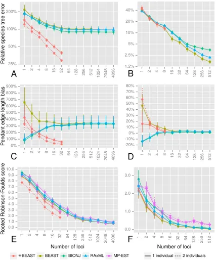
However we also found that concatenation can be far less accurate than *BEAST when

analysing simulated data designed to resemble an empirical data set from the Sino-Himalayan

plant cladeCyathophora(Eaton and Ree, 2013). For the same number of loci, *BEAST was

more accurate than concatenation at estimating species tree topologies (Figure 1.4E). For any

number of loci we tested (up to 4096), concatenation was less accurate than *BEAST using as

few as 4 loci when estimating branch lengths (Figure 1.4A). The major component of this

er-ror was the length of branches at the tips of the tree; concatenation overestimated the lengths

of tip branches by approximately 350% (Figure 1.4C).

It makes no sense to use concatenation in order to use more loci, given it will never be as

accurate as fully Bayesian MSC methods, no matter how many more loci are used. Lemmon

(20)

model choice in order to increase accuracy. That said, it would be an easier pill to swallow if

fully Bayesian MSC methods were faster, so in Chapter 2 my colleagues and I developed a

replacement for *BEAST with better performance called StarBEAST2.

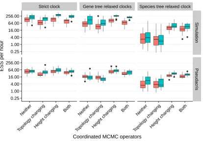
We improved the computational performance of StarBEAST2 through a combination of

analytical integration, new operators and better defaults. Support for analytical integration

sizes was first introduced in BEST (Liu, 2008), and we added it to StarBEAST2. Because

Star-BEAST2 is a Markov chain Monte Carlo (MCMC) method, it requires operators to traverse

the space of phylogenetic trees. If an operator proposes a change to the species tree that is

in-compatible with a gene tree (orvice versa), the change will be rejected. So we designed new

op-erators that make coordinated changes to the species and gene trees which will not be rejected

because of incompatibility. MCMC operators each have a default weight, and we adjusted

those weights through trial-and-error to improve performance.

The combination of those improvements increased the performance of StarBEAST2 by

more than 13-fold when analysing empirical data sets, relative to *BEAST. StarBEAST2 is

al-ready being used by researchers to infer species trees (Tougardet al., 2017; Laveret al., 2017a,b;

de Magalhãeset al., 2017; Perrot-Minnotet al., 2017) and species delimitation (Afonso Silva

et al., 2017), in some cases from previously intractable data sets of many loci and individuals (e.g. Moritzet al.2017).

0.4 Extending the multispecies coalescent

While the MSC is a more sophisticated model than concatenation, it still makes some

assump-tions which may be violated in reality or restrict the sources of data used for phylogenetic

in-ference. The latter chapters of my thesis describe extensions to the multispecies coalescent

(21)

0.4.1 Species tree relaxed clocks

Previous fully Bayesian implementations such as *BEAST and BPP assumed a fixed clock, or

relaxed clocks for gene trees that were uncorrelated with the species tree. However species

traits such as body size, and (arboreal) tree height are known to be associated with molecular

clock rates (Bromham, 2011; Lanfearet al., 2013). So when relaxed clocks are used, it makes little sense for the rate of a gene tree branch to be uncorrelated with the species tree branches it

is embedded within.

In Chapter 2 my colleagues and I introduced a new model where relative clock rates are

estimated for each species tree branch. The rate of each gene tree branch is derived from the

species tree branches it is embedded within, multiplied by a scaling factor to allow for rate

variation between loci. We called this model “species tree relaxed clocks” and implemented it

in StarBEAST2. We demonstrated that concatenation was less accurate than StarBEAST2 at

estimating per-species clock rates simulated under this model, and that using concatenation

with unphased molecular data was acutely bad at estimating those rates.

0.4.2 Multispecies network coalescent

A core assumption of the multispecies coalescent is that gene flow ceases immediately and

irrevocably after a species divergence. This assumption is violated in the case of

introgres-sion where migration/mating occurs between separate lineages of a species tree, or by

hy-brid species where a new species evolves with roughly equal genetic inheritance from parental

species.

More and more examples of introgression and hybrid species in both plants and animals are

being reported. Two North American species ofCanis,C. rufusandC. lycaon(red wolf and great lakes wolf) are the result of hybridisation between theC. lupus(grey wolf) lineage and

(22)

dis-covered for six bird species, most recentlyBranta ruﬁcollis(red-breasted goose; Ottenburghs

et al.2017). Three species ofHelianthusare the result of hybridisation betweenH. annuus

(common sunflower) andH. petiolaris(prairie sunflower), which are not even sister lineages

(Rieseberg, 1991).

Extending the MSC, the multispecies network coalescent (MSNC) introduces reticulation

nodes which have two parents and a single child, and aγvalue indicating the proportion of

inheritance from each parent (Yuet al., 2011, 2012, 2014). These reticulation nodes can model introgression and hybrid species. In Chapter 3 my colleages and I introduced a fully Bayesian

implementation of the MSNC called “SpeciesNetwork”.

This implementation is the first to use the birth-hybridization prior, which is also the first

process based prior for species networks. We demonstrated its power by confirming that the

purple cone sprucePicea purpureais a hybrid ofP. wilsoniiandP. likiangensis. Because it is

a fully Bayesian implementation, the absolute times of thePiceaspeciation and hybridisation events could be estimated as well as the network topology.

0.4.3 Fossilized birth-death-multispecies coalescent

Fully Bayesian implementations of the MSC have until now assumed that all the data are

col-lected from present-day organisms. However the fossil record is also a rich source of

mor-phological character data and time calibration. It is also, increasingly, a source of ancient

DNA (Shapiro and Hofreiter, 2014). The fossilized birth-death (FBD) process can be used

to model the evolution of species trees containing fossil data. Bayesian FBD implementations

can be used to estimate species trees containing and calibrated by fossil data (Gavryushkina

et al., 2014; Matzke and Wright, 2016). They can also be used with concatenated molecular sequence data for “total evidence” analyses (Gavryushkinaet al., 2017).

These concatenated total evidence studies will of course suffer the same problems as

(23)

of evolution that combines the FBD and MSC models. I implemented this model which we

dubbed the “MSC” in a new version of StarBEAST2 (version 14). We applied the

FBD-MSC and other models (i.e. without the FBD and/or without the FBD-MSC) to a total evidence

data set of the dog and fox subfamily Caninae.

We showed that estimated branch lengths and divergence times within Caninae differ

be-tween concatenation and the MSC, and that these differences are exactly what one expects due

to coalescent processes. Specifically, concatenation estimates of species divergence times were

consistently older than MSC estimates. The failure to account for coalescent processes

quali-tatively and quantiquali-tatively effected lineages-through-time curves of Caninae evolution when

(24)

(25)

1

Computational Performance and Statistical

Accuracy of *BEAST and Comparisons with

Other Methods

Abstract

Under the multispecies coalescent model of molecular evolution, gene trees have independent

evolutionary histories within a shared species tree. In comparison, supermatrix concatenation

methods assume that gene trees share a single common genealogical history, thereby equating

gene coalescence with species divergence. The multispecies coalescent is supported by

previ-ous studies which found that its predicted distributions fit empirical data, and that

(26)

of the multispecies coalescent, is popular but computationally intensive, so the increasing

size of phylogenetic data sets is both a computational challenge and an opportunity for

bet-ter systematics. Using simulation studies, we characbet-terize the scaling behaviour of *BEAST,

and enable quantitative prediction of the impact increasing the number of loci has on both

computational performance and statistical accuracy. Follow-up simulations over a wide range

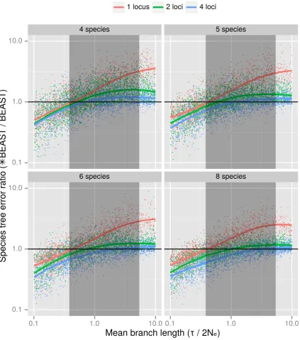
of parameters show that the statistical performance of *BEAST relative to concatenation

im-proves both as branch length is reduced and as the number of loci is increased. Finally, using

simulations based on estimated parameters from two phylogenomic data sets, we compare the

performance of a range of species tree and concatenation methods to show that using *BEAST

with tens of loci can be preferable to using concatenation with thousands of loci. Our results

provide insight into the practicalities of Bayesian species tree estimation, the number of loci

re-quired to obtain a given level of accuracy and the situations in which supermatrix or summary

methods will be outperformed by the fully Bayesian multispecies coalescent.

1.1 Introduction

In recent years a number of new techniques have applied next-generation sequencing to

phy-logenetics and phylogeography (McCormacket al., 2013). These new methods include target enrichment strategies (Mamanovaet al., 2010) like exon capture (Biet al., 2012), anchored

phylogenomics (Lemmonet al., 2012) and ultra-conserved elements (Fairclothet al., 2012), as well as RAD sequencing (Bairdet al., 2008; Daveyet al., 2011). As a result genome-wide samples of large numbers of loci from multiple individuals and multiple species have become

increasingly common. This trend is rapidly shifting themodus operandiof systematic biology from phylogenetics to phylogenomics. This move to phylogenomics has also heralded a rapid

development and uptake of species tree inference methods that acknowledge and model the

(27)

acceptance that probabilistic model-based methods are preferable, however the amount of

data produced by next-generation technologies has also spurred the development of faster

methods that do not utilize all the available data and employ statistical shortcuts such as

ad-mitting no uncertainty in individual gene trees (Kubatkoet al., 2009; Liuet al., 2009b).

1.1.1 Bayesian species tree estimation

The theory of incomplete lineage sorting and its implications for phylogenetic inference has

been appreciated for some time (Pamilo and Nei, 1988), and early approaches to applying this

theory inferred the species tree that minimizes deep coalescences using gene tree parsimony

(Maddison, 1997; Page and Charleston, 1997; Slowinski and Page, 1999). The fully

probabilis-tic application of the theory to molecular sequence analysis has only begun more recently with

the introduction of Bayesian implementations of the multispecies coalescent (Rannala and

Yang, 2003; Edwardset al., 2007; Liu, 2008; Liuet al., 2008; Heled and Drummond, 2010). This model embeds gene trees within a birth-death or pure Yule species tree, and within each

lineage (or branch) of the species tree, gene trees are assumed to follow a coalescent process

(Heled and Drummond, 2010). Prior to the development of these methods it was necessary to

assume that the history of each gene is shared and equal to the history of the species tree being

studied.

However, gene trees evolve within a species tree and the approximation of equating them

becomes increasingly problematic as one samples more loci, when in reality each have distinct

gene tree topologies and divergence times. The multispecies coalescent brings together

coa-lescent and birth-death models of time-trees into a single model. It describes the probability

distribution of one or more gene trees that are nested inside a species tree. The species tree

de-scribes the relationship between the sampled species, or sometimes, sampled populations that

have been separated for long periods of time relative to their population sizes. In the latter

(28)

The initial implementations of the multispecies coalescent made very simple assumptions

including no recombination within each locus and free recombination between loci. While

these simple assumptions can be robust to violation, including some forms of gene flow (Heled

et al., 2013) (but see Leachéet al.(2014)), researchers have begun to acknowledge that addi-tional processes (such as hybridization) may need to be incorporated (Jolyet al., 2009; Ku-batko, 2009; Chung and Ané, 2011; Yuet al., 2011; Camargoet al., 2012). A number of

sim-ulation studies have also looked at various facets of performance of Bayesian species tree

esti-mation including the influence of missing data (Wiens and Morrill, 2011), the influence of low

rates and rate variation among loci (Lanieret al., 2014) and comparisons of performance with

“supermatrix” concatenation approaches (DeGiorgio and Degnan, 2010; Largetet al., 2010; Leaché and Rannala, 2011; Bayzid and Warnow, 2013).

Although these modelling advances are exciting, in the face of a next-generation data

del-uge, this study asks and answers the following, heretofore unanswered questions: (i) How do

fully Bayesian multispecies coalescent methods scale to data sets of hundreds of loci? (ii) How

much more accurate will phylogenetic species tree estimates be with more sequence data? (iii)

When should one use a multispecies coalescent approach instead of computationally more

ef-ficient Bayesian supermatrix approaches, or summary methods which do not use all available

data? To address the first of these questions we investigate the computational performance of

the *BEAST implementation of the multispecies coalescent (Heled and Drummond, 2010), so

as to assess the feasibility of conducting phylogenomic analyses using existing computational

tools. To shed light on the second question we investigate how estimation accuracy improves

with increasing loci.

To address the final question, we investigate how the statistical accuracy of the multispecies

coalescent compares with concatenation across a broad range of conditions. We also

(29)

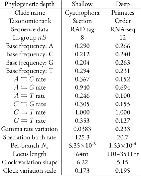
meth-ods using simulations based on two published sequence data sets; RAD tag sequences from a

study of the Sino-Himalayan plant cladeCyathophora(Eaton and Ree, 2013), and RNA-seq assemblies from a study of primates (Perryet al., 2012).Cyathophora, a section of the genus

Pedicularisoriginating in the late Miocene or the Pliocene, is probably no older than 8 Ma (Yang and Wang, 2007) and is therefore a shallow study system. In contrast primates are a

deep study system, as the oldest split in this order is estimated to have occurred in the

Creta-ceous around 80 Ma (Tavaréet al., 2002; Steiper and Young, 2006; Wilkinsonet al., 2011).

1.2 Methods

Using simulation, we investigated the trends in computational performance and statistical

accuracy of the multispecies coalescent model as implemented in BEAST 2 (*BEAST), and

its statistical accuracy relative to other methods of species tree inference. In designing these

simulation studies there were a number of parameters to consider. The key parameters that

might determine performance of inference under the multispecies coalescent are:

n: The number of species.

ni: The number of individuals sampled per species.

nl: The number of independent loci.

ns: The number of sites in a single locus.

Ne: The effective population sizes of extant and ancestral species.

τ : The branch lengths in units of time or expected substitutions.

Another factor which may influence *BEAST performance is whether the molecular

evo-lution of each locus has been more or less clock-like. Of all these parameters it is the number

(30)

nithat are largely determined by experimental design. In addition, a complete specification

of a multispecies coalescent model requires a speciation model (parameterized model of the

species tree), a substitution model (model of the relative rates and base frequencies) and a

clock model describing the absolute rate of evolution across the branches of each gene tree. In

the following sections we describe the choices of parameters, models and simulation

condi-tions for our computational experiments.

Species and gene trees for all experiments were simulated using biopy1_{, which simulates}

gene trees contained within species trees according to the multispecies coalescent process.

Sequence alignments were also simulated using biopy for experiment 1 and 2, and Seq-Gen

(Rambaut and Grassly, 1997) was used to simulate nucleotide alignments for experiment 3.

1.2.1 Experiment 1: Performance of *BEAST with increasing numbers of loci

The first set of simulations we performed was primarily aimed at understanding the effect that

increasing the number of loci has on the computational performance and statistical accuracy

of Bayesian species tree estimation. We simulated 100 random (rapidly speciating) species trees

of each of three different sizes,n = 5,8,13, using the birth-death process (Kendall, 1948; Nee

et al., 1994; Gernhard, 2008). In all cases the speciation rate wasλ = 1and the extinction rate wasµ = 0.2(nominally per million years). For 5-species trees we consideredni = 2,4,8, for

8-species treesni = 2,4and for 13-species treesni = 2. For each combination ofnandniwe

simulated up to 256 gene trees. Gene alignments were simulated from these gene trees using

an HKY substitution model (Hasegawaet al., 1985) and a strict clock. All sequences were

sim-ulated with a substitution rate of 1% per lineage per million years, a transition/transversion

ratioκof 4, equal base frequencies and a strict clock. For each *BEAST analysis, the

substi-tution rate was fixed at 1%, and a singleκvalue and set of base frequencies for all loci was

es-timated. The locus length was 200 sites each to mimic short-read next-generation sequence

(31)

data. Finally, we drew successively larger subsets of each group of alignments to form a set of

*BEAST analyses (Heled and Drummond, 2010). We considered increasing numbers of loci

on a logarithmic scale, i.e.nl ∈ {2,4,8,16,32,64,128,256}.

If the effective sample size (ESS) of either the log posterior or the age of the species tree

in an analysis was not≥200 after the initial MCMC chain was completed, we used the re-sumefunction in BEAST 2 (Bouckaertet al., 2014) to extend the MCMC chain from the final state of the previous run, until sufficient samples were obtained to achieve a minimum ESS

of 200. For each combination ofnl,nandni, MCMC chains were resumed until at least 90

out of 100 replicates had sufficient ESS values. All statistics and trees were logged at a

sam-pling rate of 1 sample per 25000 states, and the MCMC chains that needed extension were

combined into a single long chain. Pseudocode for the experimental protocol can be found in

Algorithm S1 in supplementary information.

ESS per hour was not calculated using the total CPU time for the combined chain because

resumed runs were not restricted to a single type of CPU and hence were not directly

com-parable. Instead, the initial MCMC chain for each condition and replicate was restricted to a

single type of CPU (Intel E5-2680 @ 2.70 GHz), and million states per hour of CPU time was

calculated based on the number of states and CPU time of the initial chain. To calculate ESS

per million states, the ESS of the age of the species tree was divided by the million post-burnin

states in the combined chain. To calculate ESS per hour, ESS per million states was multiplied

by million states per hour. All replicates were used to calculate average ESS rates, including

those with ESS values<200.

The main measure of error used in this study, “relative species tree error,” incorporates

both topological and branch length error by building on the previously described measure

“rooted branch score” (RBS; Heled and Bouckaert, 2013). Given two treesT1andT2, the

(32)

branch which extends rootward from the most recent common ancestor (MRCA) of a clade

is defined asb(c). Given these definitions, the rooted branch score is defined as the sum of all

absolute differences in branch lengthsb(c)between treesT1andT2:

RBS(T1, T2) = ∑

c∈C1∪C2

|b(1)(c)−b(2)(c)| (1.1)

By convention, the branch length of a clade that is missing from a tree is zero, so the

topo-logical error of absent or erroneous clades will be weighted by the true or estimated branch

length respectively. We define the relative species tree erroreT to be the posterior expectation

of the rooted branch score distanceRBSbetween the estimated species treeTˆand the true

species treeTtrue, normalized by the tree length of the true species treeLtrue:

eT = 1 k ·

∑k

i=1RBS(Ttrue,Tˆi) Ltrue

(1.2)

This measure summarizes the error over the entire posterior distribution by averaging the

RBS for eachiposterior sampleTˆidrawn from the entire set of posterior samples of sizek.

We normalize by the length of the true species tree to make the error comparable between

species trees of differing units and/or number of species. Replicates with insufficient ESS

val-ues were excluded when calculating average relative species tree error, because the posterior

distributions of species trees for those replicates might be inadequately sampled.

A post-hoc analysis was performed to investigate the residual variation in ESS rates and

rel-ative species tree error, after accounting for the number of loci, individuals and species in each

replicate. Spearman’s rank correlation was used to calculate correlation coefficients between

the residuals and various tree and alignment parameters. P-values for each correlation were

computed using asymptotictapproximation, and then corrected for multiple comparisons

(33)

Mean population size was calculated as the mean of all per-branch effective population

sizes. Species tree asymmetry is the varianceσ2

N in the number of nodes between each tip and

the tree root (Kirkpatrick and Slatkin, 1993). Mean tree height difference is the mean

differ-ence in height between each gene tree and the species tree. Mean deep coalescdiffer-ences is the mean

number of deep coalescences for each gene as calculated by DendroPy 4.0.3 (Sukumaran and

Holder, 2010). The mean parsimonious mutations is the parsimonious (minimum) number

of mutations required per site given the true gene tree, again calculated by DendroPy. Mean

variable site count is the mean number of sites per locus with more than one extant allele, and

mutations per variable site is the total number of parsimonious mutations required divided by

the total number of variable sites.

Experiment 1 was performed using the Pan cluster provided by New Zealand eScience

In-frastructure and hosted at the University of Auckland2. This high performance compute cluster provides access to Linux compute nodes with 2.7 and 2.8GHz Intel Xeon CPUs, and

approximately 8GB of RAM per CPU core.

1.2.2 Experiment 2: Comparing a Bayesian multispecies coalescent approach

with a Bayesian supermatrix approach

In the second set of simulations we compare the statistical accuracy of the multispecies

co-alescent to partitioned concatenation, both as implemented in BEAST 2. We refer to these

methods as *BEAST and Bayesian supermatrix respectively. Specifically we tested the

hypoth-esis that the comparative accuracy would depend on mean branch length in coalescent units

ofτ(2Ne)−1.

For every combination ofn = 4,5,6,8andnl = 1,2,4we simulated species trees with a

range of branch lengths in coalescent units. In order to vary branch lengths, species trees were

2_{https://www.nesi.org.nz/services/high-performance-computing/platforms}_{— accessed}

(34)

simulated with expected root heights ofR = 1₂,1,2,4,8,16(nominally in millions of years)

and population sizes chosen fromNe = 1₄,1₂,1(nominally in units of million individuals),

changing the coalescent branch length unit numerator and denominator respectively.

Addi-tional expected root heights were included where the most accurate method switches from

*BEAST to Bayesian supermatrix, to obtain denser sampling in that part of parameter space.

Species trees were generated under the pure birth Yule model (Yule, 1924). The birth rate

for each combination of parameters was set toλ = _R1 ∑n_k₌₂ 1_k, that is, the birth rate which

generates trees with an expected root height ofR. These settings roughly correspond to

mam-malian nuclear genes of species with an effective population size of one-quarter, one half or

one million individuals.

A single individual per species was simulated for all loci. We used the Jukes-Cantor

substi-tution model (Jukes and Cantor, 1969) and a strict clock model for each locus, but with rate

variation between loci. The mutation rate for the first locus was fixed atµ0 = 0.01, and the

rates for other loci drawn from the range[µ0/F, µ0 ×F]. We usedF = 3, giving a factor

of 9 between the fastest and slowest possible rates. The rate was drawn in log space, so there

is equal density of slower and faster rates aroundµ0. The number of sites per alignment (ns)

was fixed at 1000.

We generated 100 replicates for each combination ofn,nl,RandNe. For each unique

com-bination ofn,RandNeonly one set of 100 species trees was generated and used (regardless

ofnl) to minimize species tree sampling error when analyzing the effect of increasingnl. Gene

trees and extant sequences were generated separately for each replicate and for each value of

nl.

Both Bayesian supermatrix and *BEAST analyses used a Yule prior on the species tree, with

a uniform prior of[1_/

100,100]onλ, and a separate partition per locus each with a strict clock

(35)

were estimated. The *BEAST effective population size hyperparameter (popMean) was given

a uniform prior in the range[1₅,5], and all population sizes were estimated.

The Bayesian supermatrix analysis used a fixed chain length of 4 million states, sampling

every 1000 states. The *BEAST analysis used a fixed chain length of 40 million states,

sam-pling every 10,000 states. The ESS values of the posterior, likelihood and prior statistics of

each chain were estimated, and replicates where the ESS was<200 for any of those statistics

were discarded. For each combination ofn,nland method there were never more than 4%

of replicates discarded for this reason (Figure S10). As with experiment 1, this experiment was

performed using the NeSI Pan cluster.

1.2.3 Experiment 3: Many-method comparison of species tree inference using

parameters estimated from two phylogenomic data sets

The purpose of the third set of simulations was two-fold: to check that the trends in statistical

accuracy observed for the first two sets of simulations held for empirically derived simulations,

and to compare statistical accuracy across a range of species tree inference methods. To

sim-ulate more realistic trees and sequences, we derived a range of properties and phylogenetic

parameters from two empirical phylogenomic data sets for use as simulation parameters.

The biallelic species tree inference method SNAPP (Bryantet al., 2012) was used to esti-mate speciation birth rates and effective population sizes because it did not require phasing

the sequence data. To estimate base frequencies, substitution rates, between-site rate variation

and between-locus rate variation we used a Bayesian supermatrix analysis with a Yule prior on

the species tree. A detailed description of sequence data processing and SNAPP and BEAST

settings is given in supplementary information.

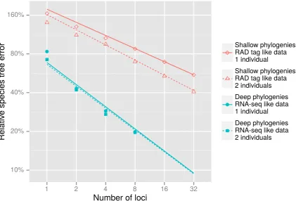
We simulated 100 replicates each of “deep” and “shallow” Yule species trees ofn = 12

andn = 8respectively, using the inferred empirical birth rates, with per-branch population

(36)

population sizes. For the deep species trees we simulated 512 gene trees, and for the shallow

species trees we simulated 4096 gene trees within each species tree, each with two individuals

per species.

For each simulated gene tree we chose a strict clock rate from the gamma distribution

de-fined by the inferred shape parameters and scale parameters. Nucleotide sequences were

sim-ulated for every locus using the empirically derived GTR+G base frequencies, substitution

rates and gamma rate variation from the applicable study. As the shallow study used 64nt

RAD tags, we picked that fixed length for sequence simulations based on that study. For

sim-ulations based on the deep study, each simulated alignment length was randomly sampled

(with replacement) from the original alignment lengths of the deep study.

Species trees were reconstructed from simulated sequences using five different multi-locus

inference methods; *BEAST, Bayesian supermatrix, MP-EST (Liuet al., 2010), RAxML ver-sion 8 (Stamatakis, 2014) and BIONJ (Gascuel, 1997). We tested *BEAST performance given

nl = 1,2,4,8for the deep study based simulations andnl = 1,2,4,8,16,32for the shallow

study based simulations. For all simulations, we tested the performance of Bayesian

superma-trix givennl = 1,2,4,8,16,32,64,128,256,512. For the deep study simulations we tested

RAxML, BIONJ and MP-EST withnl = 1,2,4,8,16,32,64,128,512. For the shallow

study simulations we also analyzednl = 1024,2048,4096. Both *BEAST and MP-EST can

infer species trees utilizing more than one individual per species, and we tested both methods

usingni = 1,2.

All GTR+G rates were estimated for *BEAST and Bayesian supermatrix analyses. For

RAxML analyses, only GTR+G substitution rates were estimated and empirical base

fre-quencies were used. Clock rate distribution parameters and clock rates for each locus were

esti-mated for *BEAST and Bayesian supermatrix analyses. Loci were not partitioned for RAxML

(37)

maxi-mum likelihood algorithm used was “new rapid hillclimbing”. Pairwise distances matrices

cal-culated by RAxML were used to generate neighbor-joining trees using the BIONJ algorithm

implemented in PAUP* version 4.0a1423_{. *BEAST and BEAST trees are implicitly rooted}

because they are ultrametric, and RAxML and BIONJ trees were midpoint rooted.

MP-EST uses gene trees as input data, which were inferred using RAxML. The same

set-tings used for RAxML species tree inference were used for gene tree inference, and gene trees

were midpoint rooted. For each replicate MP-EST was set to make 10 independent runs, and

the species tree with the highest pseudo-likelihood was retained for further analysis.

The BEAST and *BEAST chains were run on the Raijin cluster provided by the National

Computational Infrastructure4_{. This cluster provides access to Linux compute nodes with}

2.6GHz Intel Xeon Sandy Bridge CPUs, and 4GB of RAM was requested per run. Further

details of BEAST and *BEAST chains are provided in supplementary information. RAxML

and MP-EST were run on the cluster provided by the Genome Discovery Unit of the

Aus-tralian Cancer Research Foundation Biomolecular Resource Facility. Jobs on this cluster ran

on Linux compute nodes with a variety of Intel Xeon and AMD Opteron CPUs, and 2GB of

RAM was requested per RAxML or MP-EST job.

1.3 Results

1.3.1 Experiment 1: Performance of *BEAST with increasing numbers of loci

Computational performance

We evaluated the scaling of computational performance of *BEAST as a function of the

num-ber of loci analyzed. We recorded the elapsed computational time for each replicate analysis

running in a single thread. This was then used to calculate the effective number of samples per

hour (ESS per hour), to measure the computational effort required to produce a sample from

3_{http://paup.phylosolutions.com/}_{— accessed 15th December 2017}

(38)

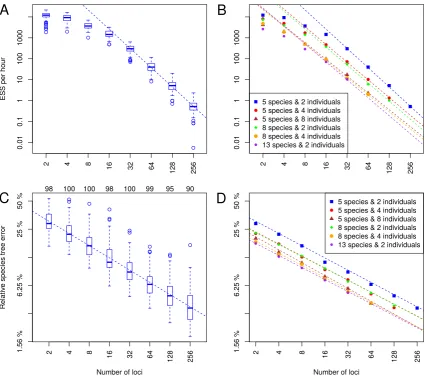
the posterior for a given number of loci. The ESS per hour relationship (Figure 1.1a,S3)

sug-gests that a power law fits the scaling of computational performance. The linear relationship

in the log-log plot indicates that a power law fits well for the range from 32 to 256 loci. We

ex-trapolate that forn = 5,ni = 2andnl ≥ 32, ESS per hour follows a power law with a slope

and intercept of−3.06±0.04and16.34±0.18respectively.

2 4 8 ₁₆ ₃₂ ₆₄

128 256 0.01 0.1 1 10 100 1000 ● ● ● ● ● ● ● ● ● ● ● ● ● ● ● ● ● ● ● ● ●

5 species & 2 individuals 5 species & 4 individuals 5 species & 8 individuals 8 species & 2 individuals 8 species & 4 individuals 13 species & 2 individuals

ESS per hour

2 4 8 ₁₆ ₃₂ ₆₄

128 256 0.01 0.1 1 10 100 1000

Number of loci

Relativ

e species tree error

2 4 8 ₁₆ ₃₂ ₆₄

128 256

1.56 %

6.25 %

25 %

50 %

98 100 100 98 100 99 95 90

Number of loci 2 4 8 ₁₆ ₃₂ ₆₄

128 256 1.56 % 6.25 % 25 % 50 % ● ● ● ● ● ● ● ● ● ● ● ● ● ● ● ● ● ● ● ● ●

5 species & 2 individuals 5 species & 4 individuals 5 species & 8 individuals 8 species & 2 individuals 8 species & 4 individuals 13 species & 2 individuals

A

C

B

[image:38.595.57.483.208.584.2]

D

Figure 1.1:Trends in ESS per hour and relative species tree error as a function of the number of loci. (a) ESS per hour

for analyses of 5 species each with 2 individuals. Each box-and-whisker shows the variance in mixing across a hundred replicate data sets for each number of loci. (b) The median ESS per hour as a function of number of loci, with trend lines for each combination of number of species and individuals per species. Solid shapes indicate the median value for each category, and regression lines were calculated using all replicates for each category. (c) Relative error for 5 species each with 2 individuals, with each box-and-whisker showing the variance in relative error between replicates. Numbers above the graph area indicate how many replicates were included for each number of loci. (d) The relative error in the estimated species tree as a function of the number of loci, with trend lines for each combination of number of species and individu-als per species. Solid shapes indicate the median value for each category, and regression lines were calculated using all replicates for each category with sufﬁcient ESS.

Applying this functional relationship, we could estimate the computational cost to analyze

(39)

in the simulation, the predicted ESS per hour is 0.54 for 256 genes, which indicates it would

take approximately 369 CPU hours to attain an ESS of 200. We can therefore estimate that a

similar analysis of 1024 loci would take roughly 1064 CPU days. Nevertheless an analysis this

size might be achieved within two months by parallelizing the problem into 20 independent

MCMC chains for two months each and discarding a few days of burnin from each of them,

to achieve on the order of ten independent samples from each chain.

Variation in ESS per hour between replicates was observed under all tested conditions

(Fig-ure S3). The slowest replicate relative to the median rate for any condition was a 5 species, 2

individuals and 256 genes outlier, 94×slower than the median rate for that combination

(Fig-ure 1.1a). This replicate would require approximately 1500 CPU days to attain an ESS of 200.

However, this was an extreme case as the next slowest replicate for that combination was

an-other outlier only 6.4×slower than the median rate, and would require only 100 CPU days to

attain the same ESS value.

The slope of the expected computational performance as a function of number of loci does

not vary with the number of species or the number of individuals (Figure 1.1b), although a

larger range ofnandniwould need to be examined to understand the scaling relationship

of computational performance with those quantities. For analyses larger than 5 species and

2 individuals, the power law range appears to begin atnl ≥ 16. Combining all simulation

results, a multiple linear regression describing a response variableY (e.g. ESS per hour) as a

function of three explanatory variables: number of locinl, number of speciesn, and number

of individuals per speciesni, can be constructed as follows:

log(Y) =β1log(nl) +β2n+β3ni+α (1.3)

Taking the ESS per hour as the response variable, the linear regression estimates of the

(40)

α = 17.98±0.13. At least within the range of parameters examined here, it appears that the

β1coefficient is not greatly influenced bynandni(Figure 1.1b).

We also considered the scaling of the number of effective samples per million states (ESS per

million states) in the MCMC analyses. This quantity is complementary to our first result; it

is easier to investigate as it does not require running all simulations on identical and dedicated

hardware. Computational time for methods like *BEAST is dominated by the phylogenetic

likelihood, which is calculated for all site patterns given a proposed tree (Yanget al., 1994).

Because *BEAST infers a separate gene tree for each locus, the time per state will be linear with

the number of loci assuming the average number of site patterns per locus is independent of

the total number of loci. This assumption of independence holds for experiment 1 because

loci were subsetted uniformly.

Adapting the terminology of Equation 1.3, the slope of ESS per hour (β1h) will be simply

related to the slope of ESS per million states (β1s):β1h = β1s + 1. However because CPU

time per site pattern depends on the specific hardware employed, the intercept of ESS per

hour (αh) cannot be predicted from that of ESS per million states (αs).

As expected, ESS per million states also exhibits a power law in the number of loci

(Fig-ure S4). By assigning the ESS per million states toY in the multiple linear regression in

Equa-tion 1.3, the estimated coefficients areβ1 = −1.87±0.02,β2 = −0.28± 0.01,β3 =

−0.24±0.01, and the estimated intercept isα = 9.07±0.12. The difference in slope

be-tween ESS per million states and ESS per hour is(−1.87)−(−2.81) = 0.94, very close to 1

as predicted. As with ESS per hour, observations used for the linear regression were restricted

tonl≥32for the 5 species, 2 individual case andnl ≥16for other cases.

Using the example of 5 species and 2 individuals, the slope and intercept are−1.97±0.04

and7.86± 0.18respectively, so the predicted ESS per million states for 256 individuals is

(41)

of 200. We can extrapolate that a similar analysis of 1024 loci would require an MCMC chain

of roughly4.3×(1024₂₅₆)1.97≈66billion states.

Statistical accuracy

We also calculated the relative error in the species tree estimate for each replicate. For some

larger analyses it was challenging to achieve acceptable ESS values for every replicate, even with

chain lengths of several billion states and access to high performance computational

infrastruc-ture. To retain the larger analyses without biasing statistical accuracy, we excluded replicates

in which the ESS of either the log posterior or the species tree age was smaller than 200. All

remaining replicates were used for a linear regression analysis of the contribution of the

num-ber of loci to relative species tree error. This analysis revealed a power law relationship from

2 to 256 loci (Figure 1.1c,S5). Given 5 species and 2 individuals, the slope and intercept are

−0.435±0.007and−0.889±0.026respectively, so the relative species tree error predicted

by the power law for 256 loci is 0.037. By extrapolation we would therefore estimate that the

relative error of a 1024 loci analysis would decrease to0.037×(1024₂₅₆)−0.435 ≈0.020.

Linear regression analysis of relative species tree error for all combinations ofnandnl

showed little variation in the trend line slope between conditions (Figure 1.1d). By assigning

the relative species tree error toY in the multiple linear regression in Equation 1.3, the

esti-mated coefficients areβ1 =−0.433±0.003,β2 =−0.066±0.002,β3 =−0.070±0.002,

and the estimated intercept isα = −0.481 ± 0.022. More details for all multiple linear

regression models are available in supplementary information. Trends in topology-only

accu-racy inferred using rooted Robinson-Foulds (rRF) scores are also presented in supplementary

information (Figure S9, Table S12).

Finally, we also analyzed the number of species tree topologies sampled in each posterior

distribution. It appears that for the analyses involving 8 and 13 species there is a rapid

(42)

it does not follow a power law (Figure S7).

Post-hoc analysis of convergence and species tree error

Experiment 1 was designed to investigate the relationship between the number of locinl,

number of speciesnand number of individualsnion ESS rates and statistical accuracy. While

these variables explained most of the variation in ESS rates and accuracy, residual variation

was present between the 100 replicates of each combination ofnl,nandni(Figure 1.1a,c).

The correlations between this residual variation and a collection of phylogenetic statistics that

could be extracted from the simulated trees and alignments were studied in a post-hoc

analy-sis.

Table 1.1:Spearman correlation of tree and alignment parameters with ESS per hour.

5n,2ni 5n,4ni 5n,8ni 8n,2ni 8n,4ni 13n,2ni

Species tree height 0.068 0.222∗∗∗ 0.362∗∗∗ −0.036 0.180∗∗∗ 0.120

Mean population size 0.075 −0.048 −0.086 −0.020 −0.101 0.121

Species tree asymmetry −0.238∗∗∗ −0.088 −0.045 −0.125∗ 0.013 −0.068

Mean deep coalescences −0.122∗∗ −0.225∗∗∗ −0.295∗∗∗ 0.020 −0.079 0.044

Mean parsimonious mutations 0.099 0.148∗∗∗ 0.122∗ −0.013 0.124∗ 0.074

Mean variable site count 0.088 0.228∗∗∗ 0.294∗∗∗ −0.045 0.146∗∗ 0.042

Mean tree height difference 0.246∗∗∗ 0.355∗∗∗ 0.315∗∗∗ 0.421∗∗∗ 0.340∗∗∗ 0.398∗∗∗

Mutations per variable site 0.030 −0.066 −0.123∗ 0.046 0.016 0.057

*:p <0.05, **:p <0.01, ***:p <0.001.

The only tree or alignment statistic that was significantly correlated with ESS per hour

con-sistently across all conditions was mean tree height difference (Table 1.1). This statistic is the

mean difference in height between each gene tree and the species tree. The positive correlation

observed for this parameter suggests that when gene trees are taller relative to the species tree,

the ESS rate will be higher and *BEAST will converge more quickly.

In contrast to ESS per hour, several statistics were consistently significantly correlated with

relative species tree error (Table 1.2). The height of the species tree and the number of variable

sites per locus were negatively correlated with relative error. This result is somewhat intuitive,

Evaluating, Accelerating and Extending the Multispecies Coalescent Model of Evolution