This is a repository copy of Towards a real-time microscopic emissions model. White Rose Research Online URL for this paper:
http://eprints.whiterose.ac.uk/2555/
Article:
Marsden, G, Bell, MC and Reynolds, SA (2001) Towards a real-time microscopic
emissions model. Transportation Research. Part D: Transport & Environment, 6 (1). 37 - 60. ISSN 1361-9209
https://doi.org/10.1016/S1361-9209(00)00012-2
[email protected] https://eprints.whiterose.ac.uk/
Reuse
Unless indicated otherwise, fulltext items are protected by copyright with all rights reserved. The copyright exception in section 29 of the Copyright, Designs and Patents Act 1988 allows the making of a single copy solely for the purpose of non-commercial research or private study within the limits of fair dealing. The publisher or other rights-holder may allow further reproduction and re-use of this version - refer to the White Rose Research Online record for this item. Where records identify the publisher as the copyright holder, users can verify any specific terms of use on the publisher’s website.
Takedown
If you consider content in White Rose Research Online to be in breach of UK law, please notify us by
White Rose Research Online
http://eprints.whiterose.ac.uk/
Institute of Transport Studies University of Leeds
This is an author produced version of an article published in Transportation Research Part D. It has been peer reviewed but does not contain the publishers formatting or pagination.
White Rose Repository URL for this paper:
http://eprints.whiterose.ac.uk/2555/
Published paper
Marsden, G.R.; Bell, M.C.; Reynolds, S.A. (2001) Towards a real-time
TOWARDS A REAL-TIME MICROSCOPIC EMISSIONS MODEL
Greg Marsden, Margaret Bell and Shirley Reynolds
ABSTRACT
This article presents a new approach to microscopic road traffic exhaust emission modelling. The model described uses data from the SCOOT demand-responsive traffic control system implemented in over 170 cities across the world. Estimates of vehicle speed and classification are made using data from inductive detector loops located on every SCOOT link. This data feeds into a microscopic traffic model to enable enhanced modelling of the driving modes of vehicles (acceleration, deceleration, idling and cruising). Estimates of carbon monoxide emissions are made by applying emission factors from an extensive literature review. A critical appraisal of the development and validation of the model is given before the model is applied to a study of the impact of high emitting vehicles. The article concludes with a discussion of the requirements for the future development and benefits of the application of such a model.
INTRODUCTION
Air pollution is estimated to cost the European Union approximately 37 BECU (0.6% of Gross Domestic Product) every year (DGVII, 1995). As much as 90% of these costs are estimated to be attributable to road transport. In recent years serious pollution episodes have become more commonplace in major cities around the world. Traffic management policies and vehicular restrictions have been introduced to minimise the severity of such episodes (Henderson and Bull, 1996). Within the UK, the Environment Act of 1995 (HMSO, 1995) has placed a mandatory requirement on local authorities to establish Air Quality Management Areas (AQMA) where air quality standards, provided by the National Air Quality Strategy (NAQS) are exceeded or are likely to be exceeded (DoE, 1997).
Within the framework described above, it has been recognised that there is a need to establish air quality monitoring and management systems. One element of such systems is a long range forecasting model that will predict the onset of periods of poor air quality that are potentially hazardous to health. In the UK, a national forecasting service has been established (Stedman et al., 1998) using data from the National Atmospheric Emissions Inventory (Goodwin et al., 1999). In addition, more detailed local models of air quality are being developed, such as the Airviro model in Leicester (Hodges and Reynolds, 1999). Traffic emissions estimation can be performed on a number of different levels, from individual vehicle emission estimation through to city wide emission estimation (Lesort et al., 1996). The level of detail selected for the emissions estimation model should correspond to the corresponding transportation system effect that is being modelled (Sturm et al., 1996).
to a vehicle emissions model capable of operating in real-time over a city centre network. Such a model will enable on-line estimation of the exhaust emission impacts of incidents on the road network and the effectiveness of dynamic emission reduction strategies to be assessed by the network operator.
The paper begins with a discussion of the main factors to be considered in exhaust emission estimation. Next, the results and implications of a previous five-year investigation into estimating CO emissions from traffic data are discussed. The rationale for the approach taken is then presented, drawing the main issues from the previous two sections together. Then, the application of real-time inductive detector loop data as an input to the vehicle simulation model used is presented. Next, a description of the vehicle simulation and exhaust emissions model is provided. Results of a comparison of queue formation at a signalised intersection using the existing model and the enhanced model are presented. Vehicle emission factors are presented and discussed before the model is tested against road-side concentration measurements over a one week period in Leicester. A small-scale application of the model to examine the importance of high emitting vehicles is then reported. The conclusions discuss the methodological problems in the validation of emissions models through the use of pollutant concentration sensors and the wider implications of this work
VEHICLE EXHAUST EMISSION ESTIMATION
The formation of vehicle exhaust emissions depends on a number of factors. Of particular importance, for a well maintained engine, is the fuel to air ratio. Modern petrol engine vehicles have electronically controlled fuel injection systems that optimise fuel flow rates to ensure stoichiometric combustion conditions (Heywood, 1988) where there is just enough oxygen available to completely oxidise the fuel. Under such conditions, Carbon Dioxide (CO2), water and Nitrogen are the main products of combustion.
Diesel engine emissions take a different profile to those from petrol engines due to the process of compression ignition that is used, rather than the spark ignition used in petrol engines. Diesel engines operate with a lower fuel to air ratio than petrol engines using lean burning fuel and air mixtures (Heywood, 1988). Principal pollutants from diesel engines are Nitrogen Oxide (NO), Particulates and Sulphur Dioxide (SO2). This paper presents a model to estimate carbon monoxide (CO) emissions, which are negligible from diesel engines, and so the process of diesel combustion is not considered further.
enriched conditions lowers the temperature of the engine slightly (through the presence of unburned hydrocarbons) to avoid damaging the catalyst and thus reduces NO2 emissions. Exhaust emissions are significantly lower than engine out emissions due to the introduction of catalytic converters. Vlieger (1997), estimated that in real traffic conditions emissions for cars with three-way catalysts were 70% lower than for non catalyst cars. Cold start emissions, before the catalyst has warmed up, are therefore particularly elevated as there are enriched, non-catalyst exhaust out emissions.
Commanded enrichment occurs during a number of circumstances. Periods of hard acceleration from idle are particularly important in urban driving. Several studies (Kelly and Groblicki (1993), Vlieger (1997), Barth et al. (1996) and Lesort et al. (1996)) have highlighted the importance of enrichment emissions to the overall emission profile for a journey. In addition, these studies suggest that current fixed bed driving cycle testing in the US and Europe do not adequately represent typical driving conditions measured on the road today. Kelly and Groblicki (1993) measured exhaust emissions during a typical journey and found that enrichment events can increase CO emissions by a factor of 2500 while hydrocarbon (HC) emissions increased by a factor of 40 and NO emissions remained unchanged. Vlieger (1997) found overall emissions from aggressive driving were up to four times higher than those from normal driving. Ross et al. (1998) showed that a brief high power commanded enrichment event can produce more CO than 500 seconds of moderate driving.
The state of maintenance of an engine has also been found to be an important variable within the fleet relating to emissions. Bishop and Stedman (1996) and Muncaster et al. (1994) have used roadside remote sensing techniques and have estimated that 10% of the vehicle fleet could be responsible for 50% of vehicle emissions (for CO). An and Ross (1996) also estimated that 40% to 50% of vehicle emissions are due to deterioration of the vehicle emission control system.
PREVIOUS RESEARCH INTO PREDICTING CO LEVELS FROM SCOOT
Reynolds (1996) investigated the development of a semi-empirical model to predict carbon monoxide levels using data from the Split, Cycle and Offset Optimisation Technique (SCOOT) demand-responsive traffic signal control system (Hunt et al., 1981). The SCOOT system measures vehicle flow arriving on a link and uses a well established traffic model to estimate vehicle flows within the network and to optimise the traffic signals to minimise delays and vehicle stops. The research by Reynolds used data on collected directly from the SCOOT traffic model (FLOW, DELAY (average delay per vehicle), STOPS (vehicle stops), CONGESTION (when traffic is stopped over the detector) and CYCLE (cycle time)) and compared this directly with carbon monoxide data from roadside pollution monitors. The monitors were located five metres upstream of the stopline and were 1.5 metres above kerb level.
Initially, the distribution of the roadside carbon monoxide data was investigated and it was found to conform to a lognormal distribution. This finding meant that statistical tests that rely on assumptions of normality had to be used with care.
Several regression techniques were explored in an attempt to produce an empirical relationship between carbon monoxide levels and SCOOT traffic parameters. These were linear and multiple regression and ARIMA (AutoRegressive Integrated Moving Average). The most promising technique was the ARIMA which could produce an adequate model to fit historic data, but could not predict future levels at all.
At this point it was decided not to continue testing empirical relationships, but instead to take an alternative approach and develop a semi-empirical model. A linear model was proposed, which used SCOOT parameters to provide estimates of the vehicle operating mode, ie whether the vehicles passing a point were idling, accelerating, decelerating or cruising.
The definitions of the SCOOT parameters STOPS, DELAY, FLOW, CONGESTION and CYCLE were used to derive estimates for the number of vehicles passing the monitor in each operating mode. The model also took into account the operating mode of vehicles travelling on the opposite side of the road and the contribution of lingering pollution from previous time periods.
The proposed model was as follows:
yt = ß0 + ß1 Mi,t + ß2 Mc,t + ß3 Ma,t + ß4 Oi,t + ß5 Oc,t + ß6 yt-1 + ß7 yt-2 + εt
where
yt = predicted pollution level at time t (ppm)
yt-1 = pollution level predicted in the previous time interval, t - 1 (ppm)
yt-2 = pollution level predicted at time t - 2 (ppm)
Mi,t = number of vehicles idling on the monitoring side of the road
Mc,t = number of vehicles cruising on the monitoring side of the road
Ma,t = number of vehicles accelerating on the monitoring side of the road
Oi,t = number of vehicles idling on the opposite side of the road
Oc,t = number of vehicles cruising on the opposite side of the road
ßn = constants
Data collected over the course of one month in Nottingham was used to derive coefficients for the model using least squares regression analysis. However, further investigation showed that some variables were collinear and the residuals were significantly autocorrelated.
Several possibilities were considered for the unexplained variance in the model. These included (urban) background levels of carbon monoxide and meteorological variables. Only the temperature was found to improve the model accuracy. The other factor that could have an effect is the emissions of the individual vehicles, and particularly the contribution of dirty vehicles. However, it was not possible to investigate this further as the SCOOT data, by its nature, does not give any information about vehicle type.
The work carried out by Reynolds left many questions unanswered. No meaningful relationships were established between the traffic model summary parameters (e.g. average delay per vehicle per cycle) and the CO levels. Had such a relationship been established, the data collection and regression procedure would have been required for every link in the network. The research described in this paper builds on the experience gained by Reynolds and addresses these issues through a different approach.
MODEL PARAMETERS
The model proposed within this paper incorporates the key findings from the studies into real-world vehicle emissions and the work performed by Reynolds. The proposed model for estimating CO emissions therefore includes factors to take account of: • Vehicle operating mode (acceleration, cruise, idle, deceleration);
• Enriched acceleration;
• State of repair of the vehicle emission control system; and • Type of engine (petrol or diesel)
The effects of cold start have not been considered as the model validation site was located on an in-bound link in a city centre where it was assumed that there would be very few vehicles operating with a cold catalyst. Typical light off times for catalysts are in the order of two minutes (Ross et al., 1998). The absence of a significant number of cold start vehicles has removed a potentially significant variable in this preliminary modelling assessment and this will need to be incorporated as the model is extended. Work is currently underway in the UK to improve the emissions factors for cold start vehicles (Cloke et al., 1998) which will support this process.
strategies may change the pattern of activity in a network and thus the instantaneous speed and acceleration profiles (Hallmark and Guensler, 1999).
The model proposed here overcomes the potential problem of inadequately representing flows within a network by using data from inductive loop detectors (rather than from the traffic model as in Reynolds (1996)), which is available in real-time from the SCOOT demand-responsive traffic signal control system. SCOOT has been installed in over 170 cities around the world (Bretherton and Bowen, 1998) and therefore, this model could see widespread application.
TRAFFIC INPUT DATA
The SCOOT traffic control system uses data on vehicle occupancy produced by inductive detector loops located at the upstream end of every link within a SCOOT network. The inductive detector loops sample for occupancy (whether a vehicle is over the loop or not) every quarter of a second registering a 1 for vehicular presence, otherwise a 0. Inductive detector loops are often used for counting vehicles on inter-urban roads where speeds are high. One study in America by Klein (1993) stated that “The accuracy of the inductive loop with respect to count was 99.4%”. This result was
consistent with that of Cherrett et al. (1996).
If vehicle arrival time is provided to a traffic simulation model then the estimation of queue formation should be enhanced. This could be improved further by estimating vehicle arrival speed and classification. The potential application of inductive loop data in providing these estimates was investigated.
Vehicle Counts from SCOOT Occupancy
Traffic travelling across SCOOT loops was monitored using video recordings made using a roadside video camera whilst collecting the raw quarter second occupancy data (Marsden, 1998). Using specially designed software, automatic data capture into computer memory directly from visual surveillance of the videos was made possible. Various detector loop configurations were studied over a range of traffic flow and on-street conditions. The real-time visually observed data were then matched with the SCOOT occupancy data and a comprehensive statistical analysis performed.
300 400 500 600 700 800 900 1000
300 400 500 600 700 800
Manual Count (vehicles/hour)
Occupancy flow (vehicles/hour)
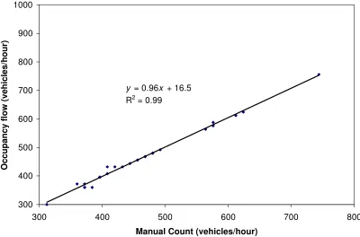
[image:9.595.95.495.89.353.2]y = 0.96x + 16.5 R2 = 0.99
Figure 1: Inductive detector loop flow against manual count flow
Inductive detector loops that span one lane of traffic produced good quality estimates of flow over a wide range of flow conditions. These were estimated to represent 70% of loops within a network. Investigations at three other sites found similar high correlation between the occupancy based and the manual count.
Vehicle Classification from SCOOT occupancy
L
2
2
v (m/s)
v (m/s)
Time
Time
loop
Ψ
δδ
l
δδ
l
δδ
t
[image:10.595.87.494.70.269.2]t
t +
Figure 2: Vehicle crossing an inductive detector loop
The zone of detection for the loop is equal to Ψ + δl, where δl is the total length
beyond the physical dimensions of the loop which has a magnetic field of sufficient magnitude to measure vehicular presence. The value of ψ for all SCOOT loops is 2m.
The time δt (seconds) which the vehicle spends over the zone of influence of the inductive detector loop (Ψ+δl) is given by:
δt δl L
v
= (Ψ+ + ) (1)
As sampling of the inductive loop occurs every quarter of a second, the number of occupancy bits registered by a vehicle (Θ) is therefore given by:
Θ = 4(Ψ+ +δl L)
v (2)
Clearly, the number of occupancy bits registered per vehicle is inversely proportional to its speed and directly proportional to the combined length of the vehicle and loop measurement zone. The theory above demonstrates that vehicles of significantly different lengths, travelling at a constant speed, will register different values of Θ.
Previous studies have used detector signal strength (Davies, 1986) and comparison of profiles of strength based on much faster sampling rates (Pye, 1984). The quarter second resolution of the 0 or 1 output from SCOOT meant classification decisions were based on different types of vehicle having significantly different lengths. Vehicle classification was based on the three groups defined as follows:
LGV commercial minibuses, 2 axle goods vehicles, short, multiple axle goods vehicles (e.g. refuse collectors); and
HGV single and double deck buses, articulated goods vehicles, long multiple axle goods vehicles.
[image:11.595.85.479.226.325.2]The distribution of the length of the UK fleet according to the three groups was obtained from vehicle manufacturer specifications and measurements of light and heavy goods vehicles made at a Post Office depot, a commercial vehicle rental company and a local chemical factory. The statistics for the resulting distributions are shown in Table 1 along with those presented by (Bell, 1977).
Table 1: Vehicle Length Information Vehicle
Classification
Mean Length (m)
(1997)
σσ length (1997)
Mean Length (m)
Bell (1977)
σσ length Bell (1977)
CAR 4.21 0.39 4.20 0.40
LGV 7.05 1.15 7.68 1.08
HGV 15.71 2.52 13.35 1.36
Traffic Queue Estimate
SIGSIM Traffic Model
Max. Car Safe Speed
Model Update
Detector Data
Car Speed Estimate
LGV Speed Estimate
HGV Speed Estimate
Vehicle Identified
Yes No
Vehicle Identified
No
Max. LGV Safe Speed
Max. HGV Safe Speed
Yes
Probabilistic Classification Decision
[image:12.595.91.503.79.449.2]SCOOT Detector Data
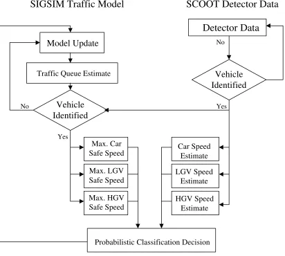
Figure 3: Flow Diagram of Vehicle Classification from Occupancy Data
99% of the traffic at the validation site was cars of which 98% were estimated correctly. Some incorrect classification of cars as LGVs resulted in a 39% overestimate in the number of LGV. There was also an 11% overestimate of HGV. However, as less than 2% of vehicles at the site were HGV and LGV these errors were not significant enough to affect the emission estimates. The observed mean and modelled mean speeds for vehicles travelling over the loop with Θ less than or equal to six was not statistically significantly different at a 95% confidence level except for Θ equal to three where there was no statistically significant difference at a 99% confidence level.
QUEUEING MODEL IMPROVEMENTS
Following the adaptation of SIGSIM to generate speed, classification and arrival time information (available from the time stamped SCOOT message) from the inductive loop detector data an assessment of the improvements to the traffic modelling was made. The car following model within SIGSIM produces estimates of the vehicle speed and acceleration every two-thirds of a second and is based on the Gipps car following algorithm (Gipps, 1981).
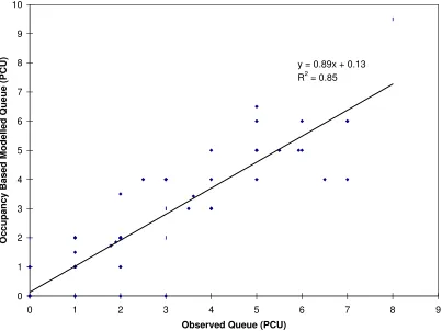
An assessment was made of the changes to the queue length at the start of the green traffic phase that resulted from using traffic characteristics from actual vehicles using the SCOOT occupancy data rather than the generic shifted negative exponential function normally used within the SIGSIM model to generate arrival rates. The assessment was performed on a single lane link. The traffic signal timings were obtained from the SCOOT system and were therefore synchronised with the vehicle occupancy data. The results of this comparison are shown in Figure 4 and Figure 5.
y = 0.89x + 0.13 R2 = 0.85
0 1 2 3 4 5 6 7 8 9 10
0 1 2 3 4 5 6 7 8 9
Observed Queue (PCU)
[image:13.595.96.499.333.635.2]Occupancy Based Modelled Queue (PCU)
y = 0.09x + 1.75 R2 = 0.02
0 1 2 3 4 5 6 7 8
0 1 2 3 4 5 6 7 8 9
Observed Queue (PCU)
[image:14.595.95.500.81.385.2]Distribution Based Modelled Queue (PCU)
Figure 5: Shifted Negative Exponential derived queue measure against observed queue
In modelling traffic at an intersection, SCOOT produces an estimate of the queue on each link. However, this measure uses the combined link profile units (thus losing the individual vehicle definition required for this work) but, more importantly, models the queue as a vertical queue at the stop-line. An assessment of SCOOT modelled queue against observed queue showed the SCOOT model to estimate just over half of the modelled queue (y = 0.50x + 0.26, R2 = 0.62). Estimates of vertical queue can be converted to a horizontal queue if the arrival flow rate is known (Bell, 1997). However, the presence of a greater degree of variation of modelled SCOOT queue at the lower levels of observed queue (where vertical and horizontal queue are closest) precluded the measure from further study.
EMISSION FACTORS
Within Europe, the COST 319 initiative (Joumard et al., 1999) has gathered together the state-of-art of vehicle emission measurement. The most significant databases that exist (e.g. Jost et al., 1992) relate to flat bed dynamometer testing where specific urban driving cycles were specified. However, despite increasing co-operation and development of databases, no suitable European database was available at the time, that took account of driving mode, enriched driving and vehicle maintenance. Much of the pioneering work in this area has been carried out in the USA.
[image:15.595.94.458.335.379.2]Stephens et al. (1996) analysed second-by-second emission data from 73 light duty cars and trucks in the USA. The results were obtained using the laboratory FTP test. Pollutant levels were given for the driving cycles split by the driving modes accelerating, decelerating, idling and cruising. The average emission concentrations at the exhaust were estimated and these are shown in Table 2.
Table 2: Modal average concentrations during warm running (Stephens et al., 1996)
Pollutant Acceleration %
Deceleration %
Cruise %
Idle %
CO 0.17 0.12 0.10 0.07
It is now widely acknowledged that the FTP driving cycle does not adequately represent enrichment events commonly found on street (EPA, 1993). The maximum acceleration in the test cycle was 3.3 mph/s (1.48m/s2). The US Environmental Protection Agency has since commissioned a review of the procedure.
A study carried out to determine a more suitable driving cycle for Los Angeles and to sample vehicle emissions for the current fleet in California is described by An et al. (1995). 165 vehicles were tested covering a wide range of models with a mileage of between 3 200 and over 200 000 miles. 41 of the vehicles tested did not have a catalytic converter. An et al. (1995) split the vehicles tested into five categories:
1. “ ‘P-cars’, representing the properly functioning cars whose tailpipe emissions are less than the 1983-1992 FTP standards, corresponding to 7.0g/mile for CO. A P-car is most likely to be a well-maintained new car with mileage less than 50 000
miles, typically the manufacturers guarantee mileage;
2. ‘M-cars’, representing cars with malfunctioning emission controls, resulted in severe tailpipe emission levels;
3. ‘D-cars’, representing cars whose emission control devices are naturally
deteriorated. A D-car is most likely to be an older car with an odometer reading
above 50 000 miles and its emission system not severely damaged;
4. ‘R-cars’, imaginary cars to represent the real-world average fleet emissions,
composed of a mixture of the P-, M-, and D- cars characteristics;
5. ‘N-cars’, representing cars without catalytic converters. All cars in the previous
Rather than approaching the modal emission definition in terms of acceleration, deceleration, cruise and idle, An et al. (1995) define the four main driving modes as:
1. stoichiometric emissions; 2. cold/warm-start emissions;
3. high-power enrichment emissions; and
4. lean-burn emissions
[image:16.595.92.491.277.354.2]The stoichiometric operating condition represents the behaviour of the vehicle throughout the drive cycle with the exception of start-up events and brief enrichment periods. Table 3 shows the correlation between the four driving states defined above for the traditional engine driving modes.
Table 3: Correlation between emission modules and driving modes (An et al., 1995)
idle start cruise acceleration deceleration
stoichiometric ++ ++ ++ +
cold/warm start +++
enrichment +++ + ++ +
lean-burn ++ ++ +++
Where:
+++ represents strong correlation; ++ represents moderate correlation; and + represents weak correlation.
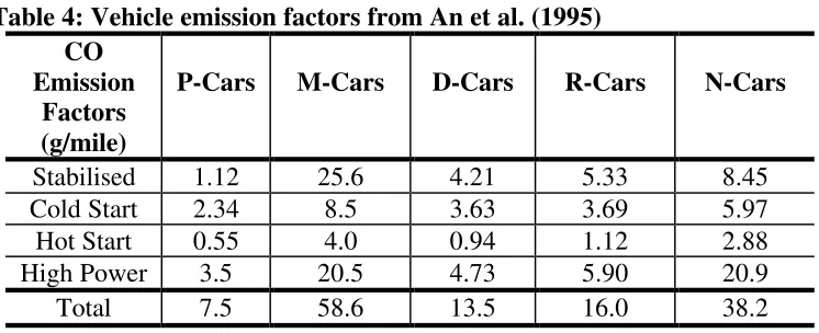
Estimated emissions factors for each of the five vehicle types listed above were developed for CO, HC and NOx. The CO emissions factors for each of the five vehicle
types are shown below in Table 4. Stoichiometric and stabilised operation and enrichment and high power operation are analogous.
Table 4: Vehicle emission factors from An et al. (1995) CO
Emission Factors (g/mile)
P-Cars M-Cars D-Cars R-Cars N-Cars
Stabilised 1.12 25.6 4.21 5.33 8.45
Cold Start 2.34 8.5 3.63 3.69 5.97
Hot Start 0.55 4.0 0.94 1.12 2.88
High Power 3.5 20.5 4.73 5.90 20.9
Total 7.5 58.6 13.5 16.0 38.2
[image:16.595.94.467.504.656.2]types to be considered were obtained from the Stephens factors by multiplying the ratio of the average vehicle to the vehicle type considered as follows:
Stabilised Stabilised m
m
Rcar Pcar E
E (PCar)= (Stephens)× (3)
A further extension to this was the introduction of a harsh acceleration mode. The value for harsh acceleration was obtained by multiplying the acceleration figure for the vehicle engine type by the ratio of high power emissions to the stabilised emissions from Table 4.
The definitions of the boundaries between driving modes were taken from Stephens et al. (1996) for acceleration, deceleration, cruise and idle. The definition of enriched driving was found to vary between studies. An et al. (1995) estimated that enriched engine performance occurs 2.4% of the time, Kelly and Groblicki (1993) estimated that such conditions exist for 1.2% of a typical urban journey whilst Ross et al. (1998) estimate commanded enrichment for 3.6% of the time. The acceleration distributions within SIGSIM are specified by parameter values provided by the user. Although they may not be truly representative of 1999 traffic behaviour, we adopted Gipps' original values for the model. An examination of the acceleration rates produced by the SISGSIM traffic model for a sample data run was used to estimate the 98th percentile of acceleration levels. Accelerations above this value (2.24m/s2) were taken to result in enriched operation. This compares to a threshold value of 2.69m/s2 estimated by Hallmark and Guensler (1999).
Occupancy Data Vehicle Generation
Figure 3
Update Vehicles
New Speed New Acceleration
Driving Mode
Emission
Emission Factor Location
Assign Engine Type (Petrol/Diesel) and Emissions Type (P, M, D, N)
Figure 6: SIGSIMPLE Schematic Diagram
METHODOLOGICAL APPROACH FOR THE EMISSIONS MODEL VALIDATION
The limitations of using USA based emission factors in a UK study are acknowledged. Perhaps it is reasonable to assume that the relative levels of pollutant emission for the different vehicle modes are similar. Although the absolute emission levels may be incorrect, the shape of the distribution of emissions will be the same. Another complication in validating the emissions estimated by the model is that due to chemical reactions and dispersion, pollutant concentrations measured at the roadside are not the same as emissions.
A further complication occurs if any attempt is made to compare the level of emissions predicted for a period of time with that measured simultaneously in the same period of time. This is created by the contribution to emissions of gross emitting vehicles. Whilst 10% of vehicles can be labeled as gross polluters (Bishop and Stedman, 1996), the actual labeling of vehicles is random (and this is unlikely to correspond to actual passing gross emitting vehicles). The same will apply to cold start vehicles when they are incorporated.
This study was also restricted to the estimation of CO emissions for the reasons described in the section on vehicle exhaust emissions estimation. An assumption was made that all light and heavy goods vehicles were diesel and therefore contributed a negligible amount of CO. A manual traffic count of the proportion of diesel cars found in the validation site was undertaken. Observations of over 3500 vehicles showed 17% of passenger cars to be diesel vehicles.
The vehicle split between car and light and heavy goods vehicles was determined using the SCOOT occupancy data. Assumptions about the state of repair of the engines for cars within the catalyst classification were taken to be those from An et al. (1995). The proportion of non-catalyst cars was estimated from observations of the vehicle fleet age and knowledge of the rate of introduction of catalytic converters. For the research described within this paper, the split between engine types within the car category was therefore estimated to be:
• 36% non-catalyst petrol-engine cars • 14% P-type cars;
• 8% M-type cars; • 25% D-type cars; and • 17% diesel cars.
MODEL ASSESSMENT
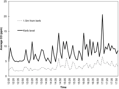
0 5 10 15 20 25
12:05 12:20 12:35 12:50 13:05 13:20 13:35 13:50 14:05 14:20 14:35 14:50 15:05 15:20 15:35 15:50 16:05 16:20 16:35 16:50 17:05 17:20 17:35 17:50
Time
Average CO (ppm)
1.5m from kerb
[image:20.595.95.487.82.378.2]Kerb level
Figure 7: Comparison of ground level and 1.5m above ground CO concentration measurements
Other analysis from Marsden (1998) did not show any evidence of significant re-circulation of pollutants at the site (the site is not a narrow canyon). It was also found that the wind had a significant effect on pollutant concentration readings at 1.5m that was not evident at ground level. Whilst the future development of the model would incorporate a dispersion model to provide estimates of pollutant concentrations, as well as emissions, a limited validation of the model was attempted using the ground level CO monitors. The CO sensors were used to measure pollutant concentrations at floor level over a period of one week. SCOOT occupancy data was collected simultaneously. Details of the survey periods and sensor locations are shown in Table 5.
Table 5: Validation survey details
Date Monitor Location Survey Period Duration
(hours:mins) 28th July 1997 5m from stop-line 13:10 – 16:00 2:50 29th July 1997 5m from stop-line 12:00 – 18:00 4:00 5m from stop-line 11:40 – 14:00 2:20 30th July 1997
25m from stop-line 11:40 – 13:45 2:05 31st July 1997 5m from stop-line 12:00 – 18:00 6:00 1st August 1997 5m from stop-line 11:00 – 17:00 6:00
[image:20.595.85.513.589.714.2]minute by minute basis showed that on average, consecutive minute readings differ by between 12.9% and 19.6% with maximum differences of between 66.7% and 126%. This shows the importance of modelling exhaust emissions every traffic signal cycle. However, given the limitation of the time resolution of the pollutant sensor, the predicted exhaust emissions (estimated every 0.67 seconds) were also summed up and aggregated to a five-minute average. The five-minute averages were calculated for each 10 metre section of road. A sample output from the SIGSIMPLE is shown in Figure 8.
0 1 2 3 4 5 6 7 8 9
07:35 07:55 08:15 08:35 08:55 09:15 09:35 09:55 10:15 10:35 10:55 11:15 11:35 11:55 12:15 12:35 12:55 13:15 13:35 13:55 14:15
Time of Day
5 minute average CO level (%)
Figure 8: Sample output of the exhaust emissions estimation model
The distributions of estimated emissions were compared directly to the pollutant concentration measurements taking no account of dispersion of the emissions. The hypothesis was made, in the light of the comparative study of monitor types and locations, that monitoring readings at kerb level would be related to exhaust out emissions. The units of estimated emissions and pollutant concentrations are different so the distributions were standardised before comparison. Spiegel (1992) states that “These (standardised variables) are of great value in the comparison of distributions.” Standardising two samples (such as observed and modelled CO) gives
both samples the same x-axis scale and the same mean (zero). Spiegel (1992) defines a standardised variable as:
z X X s
where:
X is the variable (in this case CO); X is the sample mean; and
s is the sample standard deviation.
[image:22.595.97.478.400.691.2]The maximum number of observations available to compare the measured with the modelled results was 72 (all day 31st July). This sample size makes the 2 test unsuitable for comparing the shape of the distributions. The Kolmogorov-Smirnov test is more appropriate for testing discrete or finely aggregated distributions. This test is employed for all further comparisons. The Kolmogorov-Smirnov test assesses the differences in cumulative distribution functions. The critical value for the Kolmogorov-Smirnov test is obtained from look-up tables (e.g. Kanji, 1993) where the number of degrees of freedom equals the combined measured and modelled sample size. The null hypothesis that the modelled standardised distribution is not different from the measured standardised distribution was tested. The 95% confidence limits were calculated by adding to and subtracting from the standardised distribution line, the 95% confidence measure.
Figures 9 shows a typical plot of the standardised distributions for 31st July at the measurement point 5m and the modelling section 0 to 10m. Figure 10 shows the plot for the whole week of surveys combined. Table 6 shows the results for the whole week of surveys.
-0,2 0 0,2 0,4 0,6 0,8 1 1,2
-2,1 -1,8 -1,5 -1,2 -0,9 -0,6 -0,3
0
0,3 0,6 0,9 1,2 1,5 1,8 2,1 2,4 2,7 3 3,3
Standardised CO
Cumulative frequency
Standardised observed Standardised modelled Lower 95% confidence limit Upper 95% confidence limit
-0,2 0 0,2 0,4 0,6 0,8 1 1,2
-2,2 -1,9 -1,6 -1,3 -1 -0,7 -0,4 -0,1 0,2 0,5 0,8 1,1 1,4 1,7
2
2,3 2,6 2,9 3,2 3,5
Standardised CO
Cumulative frequency
[image:23.595.97.480.81.378.2]Standardised observed Standardised modelled Lower 95% confidence limit Upper 95% confidence limit
[image:23.595.90.511.459.597.2]Figure 10: Standardised Observed (5m) and Modelled (0 to 10m) CO levels – whole week combined
Table 6: Minimum and maximum differences between observed and modelled standardised CO distributions
Kolmogorov-Smirnov test
Standardised (observed - modelled)
Date 95% critical value min. Max.
28th July 1997 ±0.26 -0.21 0.29
29th July 1997 ±0.19 -0.31 0.31
30th July 1997 ±0.24 -0.13 0.13
31st July 1997 ±0.11 -0.08 0.13
1st August 1997 ±0.12 -0.06 0.11
All ±0.07 -0.07 0.06
-0,4 -0,2 0 0,2 0,4 0,6 0,8 1 1,2 1,4
-1,3 -1,1 -0,9 -0,7 -0,5 -0,3 -0,1 0,1 0,3 0,5 0,7 0,9 1,1 1,3 1,5 1,7 1,9 2,1 2,3
Standardised CO
Cumulative frequency
[image:24.595.96.479.80.374.2]Standardised observed Standardised modelled Lower 95% confidence limit Upper 95% confidence limit
Figure 11: Standardised Observed (25m) and Modelled (20 to 30m) CO levels 300797
The results show that the distributions of modelled standardised emissions are not statistically significantly different from the measured standardised pollution distribution to the level of 95% confidence on two of the five survey periods. The differences on two of the other survey periods are small and the combined distributions for the five survey periods are not statistically significantly different. Whilst this does not validate the model, it lends confidence to the approach taken to assess exhaust emissions against measured kerbside, ground level measurements and of determining emissions according to driving mode.
The approach taken in attempting to validate the model requires further investigation, particularly with regard to the application of this model at a site independent of any of the calibration procedures. However, whilst the majority of the monitoring comparisons were performed at the 5m measurement point, it was encouraging that the mid-link standardised modelled and measured distributions were also not statistically significantly different at a 95% level of confidence. The approach described to assess the quality of the emissions estimates using kerb level monitors could also be applied to a number of other in-use emissions estimation models which have yet to undergo such a validation, due mainly to the methodological difficulties that this study has attempted to overcome.
The approach described in this paper has significant advantages over that currently being proposed for use within SCOOT (Bretherton and Bowen, 1998) which relies on average speed estimates over the link. To fully understand the benefits of introducing new technologies such as electric vehicles or semi-automatic driving, where changes to the driving profile and in particular acceleration of vehicles are significant, it is essential to have a model capable of modelling the impacts of such changes. The model evaluation presented here would benefit from a further independent validation of the traffic model with data from an Instrumented Vehicle (Brackstone et al., 1999).
Further development of the vehicle prediction model could also be undertaken. However, video image technology or new intelligent loop classification systems may offer a better long-term alternative identification methodology for emissions estimation. Number plate recognition could also be linked to the vehicle licensing database to provide further information about the vehicle.
APPLICATION OF THE MODEL
The SCOOT traffic control system operates in real-time over large parts of an urban centre network. The model proposed in this paper could operate in a number of ways with the SCOOT system:
1. As a real-time emissions estimator which could feed directly in to air quality models or as a permanent monitor of the evolution of levels of emissions over time as new strategies are introduced on the network;
2. as a strategic assessment tool. University College London has developed the SIGSIM model to run using parallel computing techniques. A virtual SCOOT network could be operated in conjunction with SIGSIMPLE such that different traffic control scenarios could be modelled in response to traffic incidents or forecast air quality episodes to minimise a particular target pollutant;
3. as a wider policy assessment tool to examine the emissions effects of the introduction of new engine technology or new vehicle-control algorithms.
A trial application of the model to examine the comparative benefits of the gradual reduction of the number of non-catalytic converter equipped vehicles and the removal of the 10% of high emitting vehicles from the fleet was undertaken. The modelling required an alteration of the vehicle fleet composition.
Table 7: Reductions in emissions estimated from strategies 1 to 3 over base case Scenario 1
Change over base (%)
Scenario 2 Change over base (%)
Scenario 3 Change over base (%) Location
µµ σσ max µµ σσ max µµ σσ max
0-10m 35.5 13.6 10.3 35.1 42.1 43.4 67.2 69.0 65.8 10-20m 30.9 6.5 7.1 33.3 40.0 49.9 65.3 66.9 67.7 20-30m 40.3 36.7 35.4 36.9 44.9 51.4 66.3 68.7 69.9 30-40m 36.6 29.6 32.7 34.8 38.0 46.6 65.1 65.3 68.2 40-50m 36.2 22.9 28.6 35.7 43.4 44.4 66.4 69.5 72.3
The results from Table 7 show that the magnitude of the change in the mean value of emissions brought about by scenarios one and two is similar, ranging between 30.9% and 40.3%. It has been estimated that 10% of vehicles produce 50% of CO emissions (Bishop and Stedman, 1996). The results show that a reduction in emissions of 33.3% to 36.9% could be achieved if these vehicles were all identified and replaced by clean vehicles (scenario two). A reduction of 40% would perhaps be expected if the 10% of P-type vehicles were to represent 10% of the emissions for the fleet. However, it is intuitively reasonable that a 40% reduction is not achieved because the data to determine the relative contribution of clean and dirty vehicles has been measured using remote sensing techniques. Such techniques require vehicles to drive by whilst cruising at a constant velocity. This underestimates the contribution of enriched emissions from properly functioning vehicles during acceleration, (which are almost three times as high as stabilised emissions as shown in Table 4) and overestimates the contribution of dirty vehicles as cruising emissions for high emitters are higher than the corresponding acceleration emissions (Table 4). This finding is supported by a previous review carried out by the Sierra Research Foundation (Austin et al., 1994).
The comparison of maximum values and standard deviations shows a more clear difference between the strategies, particularly in the areas closest to the stop-line. Removing the high emitters from the fleet reduces the standard deviation of the emissions estimated by between 38% and 44.9% and reduces the maximum emissions levels estimated by between 43.4% and 51.4%. Removing only non-catalyst vehicles from the fleet alone provides reductions in standard deviation of the emissions of between 6.5% and 36.7% and reductions of the maximum value of between 7.1% and 35.4%. The role of dirty vehicles is clearly important in determining the maximum emissions on a road section, particularly when idling, which is most likely to occur near the stop-line, supported by the scenario one results for 0 to 10m and 10 to 20m.
CONCLUSIONS
A microscopic emissions model for estimation of CO exhaust emissions has been developed that could operate on-line in real-time and off-line, as a strategy assessment tool. The model can use input from the SCOOT demand-responsive traffic control system to identify vehicle type and estimate speed of vehicles as they pass over the inductive detector loops located toward the upstream end of each link within a SCOOT network.
The exhaust emissions estimates have been compared with floor level kerbside CO concentration measurements. No statistically significant differences were found between the standardised distributions of measured concentrations and modelled emissions over five days of surveys. Further testing of the methodology at independent sites is required to prove the validity of the model. However, this study has attempted to develop a methodology for validating microscopic emissions models without the incorporation of dispersion modelling techniques. Kerbside, ground-level pollution sensors were found to be less affected by dispersion and local weateher conditions than those at face height.
Microscopic modelling of traffic flow and driving mode plays an essential part in the assessment of the potential of and implementation of new traffic demand management measures that will significantly alter the driving profile over an area. Macroscopic traffic models based simply on average speed and flow levels will not adequately model the detail of the effects of new technologies on driving patterns. Several studies have highlighted the importance of driving modes and acceleration to exhaust emissions and this paper has demonstrated the feasibility of modelling these factors.
An exploratory application of the model has reinforced the need to improve the detection and maintenance of high emitting vehicles which were shown to be responsible for significantly elevating overall CO emissions, particularly during idling ad acceleration periods which predominate near the stop-line, where pedestrian exposure may be highest. Further application of the model using parallel-computing techniques has been proposed to enable on-line emissions control strategies to be implemented.
ACKNOWLEDGEMENTS
REFERENCES
Algers, S., Bernauer, E., Boero, M., Breheret, L., DiTaranto, C., Dougherty, M., Fox, K. and Gabard, J. (1997) Review of Micro-simulation models. SMARTEST EU Fourth Framework Project Deliverable D3, University of Leeds Institute for Transport Studies.
An, F., Barth, M. and Ross, M. (1995) Vehicle Total Life Cycle Exhaust Emissions .SAE Technical Paper 951856, SAE, Warrendale, PA 15096-0001 USA
An, F. and Ross, M. (1996) A Simple Physical Model for High Power Enrichment Emissions. Journal of the Air and Waste Management Association, 46, 216-223.
Austin, T.C., DeGenova, F.J. and Carlson, T.R. (1994) Analysis of the Effectiveness and Cost-Effectiveness of Remote Sensing Devices. Report SR 94-05-05, Sierra Research Inc, Sacramento, USA.
Barth, M., An, F., Norbeck, J. and Ross, M. (1996) Modal Emissions Modeling: A Physical Approach. Transportation Research Record, 1520, 81-88.
Bell, M. C. (1977) Queues at Junctions Controlled by Traffic Signals. Research Report 26, Transport Operations Research Group, Newcastle-upon-Tyne.
Bell, M. C., Evans, R. G., Reynolds, S. A., Boddy, R. E. and Hill, I. (1996a) An Introductory Guide to the Instrumented City Facility. Traffic Engineering and Control, 37 (12), 698-703.
Bell, M. C., Reynolds, S., Gillam, W. J., Berry, R. and Bywaters, I. (1996b) Integration of Traffic and Environmental Monitoring and Management Systems. 7th International Conference on Road Traffic Monitoring and Control, 1 (1), London.
Bell, M. G. H. (1997) In Transport Planning and Traffic Engineering, Chapter 26 (Ed, O'Flaherty, C. A.) Arnold, London.
Bishop, G. A. and Stedman, D. H. (1996) Measuring the Emissions of Passing Cars.
Accounts of Chemical Research, 29, 489-495.
Brackstone, M., McDonald, M. and Sultan, B. (1999) Dynamic Behavioural Data Collection Using an Instrumented Vehicle. Transportation Research Record, 1689,
9-17.
Bretherton, R. D. and Bowen, G. T. (1998) SCOOT Version 4. 9th International Conference on Road Transport Information and Control, 1 (1), London, 104-108.
Cloke, J., Boulter, P., Davies, G. P., Hickman, A. J., Layfield, R. E., McRae, I. S. and Nelson, P. M. (1998) Traffic Management and Air Quality Research Programme. TRL Report PR SE/493/98, Transport Research Laboratory, Crowthorne.
Davies, P. (1986) In Information Technology Applications in Transport (Eds,
P.Bonsall and M.Bell) VNU Scientific Press, pp. 11-40.
DGVII (1995) Towards Fair and Efficient Pricing in Transport. COM(95)691/Provisional, European Commission, Brussels.
DoE (1997) The United Kingdom National Air Quality Strategy. The Stationery Office, London.
EPA (1993) Federal test Procedure Review Project: Preliminary Project Report. EPA 420-R-93-007, Environmental Protection Agency, Washington DC.
Gipps, P. G. (1981) A Behavioural Car-Following Model for Computer Simulation.
Transportation Research B, 15, 105-111.
Goodwin, J. W. L., Salway, A. G., Eggleston, H. S., Murrells, T. P. and Berry, J. E. (1999) National Atmospheric Emissions Inventory: UK Emissions of Air Pollutants 1970 to 1996. AEA Technology NETCEN, Oxford.
Hallmark, S. L. and Guensler, R. (1999) Comparison of Speed/acceleration Profiles from Field Data with NETSIM Output for Modal Air Quality Analysis of Signalized Intersections. 78th Annual Meeting of Transportation Research Board, CD
Washington D.C.
Henderson, G. and Bull, M. (1996) Policy Options for Improving Air Quality: The relationship Between Transport Policies and Air Quality. 24th European Transport Forum, C, Brunel University.
Heywood, J. B. (1988) Internal Combustion Engine Fundamentals, McGraw-Hill.
HMSO (1995) The Environment Act. Parliamentary Legislation, HMSO, London.
Hodges, N. and Reynolds, S. A. (1999) Leicester Demonstrator. Effect Project Launch Seminar, Leicester City Council, Leicester.
Hunt, P. B., Robertson, D. I., Bretherton, R. D. and Winton, R. I. (1981) SCOOT - a Traffic Responsive Method of Co-ordinating Signals. Laboratory Report LR1014, Transport and Road Research Laboratory, Crowthorne.
Jost, P., Hassel, D., Weber, F. J. and Sonnborn, K. S. (1992) Emission and Fuel Consumption Modelling Based on Continuous Measurements. Deliverable 7, TÜV Rhineland, Cologne.
Kanji, G. K. (1993) 100 Statistical Tests, SAGE Publications.
Kelly, N. A. and Groblicki, P. J. (1993) Real-world Emissions from a Modern Production Vehicle Driven in Los Angeles. Journal of the Air and Waste Management Association, 43, 1351-1357.
Klein, K. A. (1993) Traffic Parameter Measurement technology Evaluation. IEEE-IEE Vehicle Navigation and Informations Systems Conference, Ottowa, 529-533.
LeBlanc, D. C., Meyer, M. D., Saunders, F. M. and Mulholland, J. A. (1994) Carbon Monoxide Emissions from Road Driving: Evidence of Emissions Due to Power Enrichment. Transportation Research Record, 1444, 126-134.
Lesort, J. B., Taylor, M. A. P. and Young, T. M. (1996) Developing a Set of Fuel Consumption and Emissions Models For Use in Traffic Network Modelling.
Proceedings Of The 13th International Symposium On Transportation And Traffic Theory, Lyon, France, 289-314.
Marsden, G. and Bell, M. C. (1999) Road Traffic Pollution Monitoring and Modelling Tools and the UK National Air Quality Strategy. Submitted to Local Environment.
Marsden, G. R. (1998) Towards a Real-time Road Traffic Pollution Estimator. PhD. Thesis. Department of Civil Engineering, University of Nottingham, Nottingham.
Muncaster, G. M., Hamilton, R., Revitt, D. M., Stedman, D. H. and Vanke, J. (1994) Individual Emissions from On-road Vehicles. International Symposium on Advanced Transportation Applications: The Motor Vehicle and the Environment - Demands of the Nineties and Beyond.
Pye, K. J. (1984) Vehicle Classification using Digital Inductive Detector Loop Vehicle Detectors. Australian Road Research Board Conference, 12, 208-215.
Reynolds, S. A. (1996) Monitoring and prediction of air pollution from traffic in the urban environment. PhD. Thesis. Department of Civil Engineering, University of
Nottingham, Nottingham.
Ross, M., Goodwin, R., WAtkins, R., Wenzel, T. and Wang, M. Q. (1998) Real-world Emissions from Conventional Passenger Cars. Journal of the Air and Waste Management Association, 48, 502-515.
Shearn, S., Wood, K. and Bowen, G. T. (1997) The Estimation of Vehicle Emissions using SCOOT - Final Report. Project Report - Unpublished PR/TT/016/97, Transport Research Laboratory, Crowthorne.
Silcock, J. P. (1993) SISGSIM Version 1.0 Users Guide. User Guide University of London Centre for Transport Studies, London.
Stedman, J. R., Espenhahn, S. E. and Willis, P. G. (1998) Air Pollution Forecasting in the United Kingdom: 1997. Contract Report EPG 1/3/59, AEA Technology NETCEN.
Stephens, R. D., Cadle, S. H. and Qian, T. Z. (1996) Analysis of Remote Sensing Errors of Omission and Comission Under FTP Conditions. Journal of the Air and Waste Management Association, 46, 510-516.
Sturm, P. J., Pucher, K., Sudy, C. and Almbauer, R. A. (1996) Determination of Traffic Emissions - Intercomparison of Different Calcualtion Methods. The Science of the Total Environment, 189/190, 187-196.