Computer viruses:
from theory to applications
Chef du laboratoire de virologie et cryptologie
École Supérieure et d'Application des Transmissions
B.P. 18
35998 Rennes Armées
et INRIA-Projet Codes
ISBN 10: 2-287-23939-1 Springer Berlin Heidelberg New York
ISBN 13: 978-2-287-23939-7 Springer Berlin Heidelberg New York
© Springer-Verlag France 2005 Printed in France
Springer-Verlag France is a member of the group Springer Science + Business Media
First edition in French © Springer-Verlag France 2004 ISBN : 2-287-20297-8
Apart from any fair dealing for the purposes of the research or private study, or criticism or review, as permitted under the Copyright, Designs and Patents Act 1998, this publication may only be reproduced, stored or transmitted, in any form or by any means, with the prior permission in writing of the publishers, or in the case of reprographic reproduc-tion in accordance with the terms of licenses issued by the copyright. Enquiry concerning reproducreproduc-tion outside those terms should be sent to the publishers.
The use of registered names, trademarks, etc, in this publication does not imply, even in the absence of a specific sta-tement, that such names are exempt from the relevant laws and regulations and therefore free for general use.. SPIN: 11361145
Preface
“Viruses don’t harm, ignorance does. Is ignorance a defense?”
herm1t
“[. . . ] I am convinced that computer viruses are not evil and that programmers have a right to create them, to possess them and to experiment with them . . . truth seekers and wise men have been per-secuted by powerful idiots in every age . . . ´’
Mark A. Ludwig
Everyone has the right to freedom of opinion and expression; this right includes freedom to hold opinions without interference and to seek, receive and impart information and ideas through any media and regardless of frontiers.
Article 19 of Universal Declaration of Human Rights
The purpose of this book is to propose a teaching approach to under-stand what computer viruses1 really are and how they work. To do this, three aspects are covered ranging from theoretical fundamentals, to prac-tical applications and technical features; fully detailed, commented source
1 We will systematically use the plural form “viruses” instead of the litteral one “virii”.
codes of viruses as well as inherent applications are proposed. So far, the applications-oriented aspects have hardly ever been addressed through the scarce existing literature devoted to computer viruses.
The obvious question that may come to the reader’s mind is: why did the author write on a topic which is likely to offend some people? The motivation is definitely not provocation; the original reason for writing this book comes from the following facts. For roughly a decade, it turns out that antiviral defense finds it more and more difficult to organize and quickly respond to viral attacks which took place during the last four years (remember the programs caused by the release of worms, such asSapphire,BlasterorSobig, for example). There is a growing feeling among users – and not to say among the general public – that worldwide attacks give antivirus developers too short a notice. Current viruses are capable of spreading substantially faster than antivirus companies can respond.
As a consequence, we can no longer afford to rely solely on antivirus programs to protect against viruses and the knowledge in the virus field is wholly in the hands of the antiviral community which is totally reluctant to share it. Moreover, the problems associated with antiviral defense are complex by nature, and technical books dedicated to viruses are scarce, which does not make the job easy for people interested in this ever changing field.
For all of these reasons, I think there is a clear need for a technical book giving the reader knowledge of this subject. I hope that this book will go some way to satisfying that need.
This book is mainly written for computer professionals (systems adminis-trators, computer scientists, computer security experts) or people interested in the virus field who wish to acquire a clear and independent knowledge about viruses as well as incidently of the risks and possibilities they repre-sent. The only audience the book is not for, is computer criminals, unfairly referred as “computer geniuses” in the media who unscrupulously encourage and glamorize them somehow. Computer criminals have no other ambition than to cause as much damage as possible, which mostly is highly prejudi-cial to everyone’s interests. In this situation, it is constructive to give some essential keys that open the door to the virus world and to show how wrong and dangerous it is to consider computer criminals as “geniuses”.
fa-mous French writer, F. Rabelais in 1572, “science without conscience is the soul’s perdition”.
The problem lies in the fact that users (including administrators) are doomed, on the one part, to rely on antivirus software developed by profes-sionals and, on the other part, to be subjected to viral programs written by computer criminals. Computers were originally created to free all mankind. The reality is quite different. There is no conceivable reason why some self-proclaimed experts driven for commercial interests should restrict computer knowledge. The latter should not be the exclusive domain of the antiviral programs developers.
In this respect, one of the objectives of the book is to introduce the reader to the basic techniques used in viral programs. Computer virology is indeed simply a branch of artificial intelligence, itself a part of both mathematics and computer science. Viruses are only simple programs, which incidentally include specific features.
However uncomfortable that may be for certain people, it is easy to pre-dict that viruses will play an important role in the future. The point of this book is to provide enough knowledge on viruses so that the user becomes self-sufficient especially when it comes to antiviral protection and can find a suitable solution whenever his antiviral software fail to eradicate a virus. Whether one likes it or not, computer virology teaching is gradually becom-ing organized. At Calgary University, Canada, computer science students have been offered a course in virus writing since 2003, which as might be expected, has set off a wave of criticism within the antivirus community (the reader will refer to [138, 139, 147–149] for details).
For all of the above-mentioned reasons, there is no option but to work on raw material: source codes of viral programs. Knowledge can only gained through code analysis. Here lies the difference between talking about viruses and exploring them. Studying viruses surely will not make you a computer vandal for all that, on the contrary. Every year, thousands of people are studying chemistry. As far as I know, they rarely indulge in making chem-ical weapons once they have received their Ph. D degree. Should we ban chemistry courses to avoid potential but unlikely risks even though they do exist and must be properly assessed? Would it not be a nonsense to give up the benefits chemistry brings to mankind? The same point can be made for computer virology.
by a fallacious marketing, because some of them are reluctant to disseminate all relevant technical information, users are inclined to think that antivirus software is a perfect protection, and that the only thing to do is to buy any-one of them to get rid of a virus. Unfortunately, the reality is quite different since most antiviral products have proved to be unreliable. In practice, it is not a good thing to rely solely on commercial anti-virus programs for pro-tection. It is essential that users get involved in viral defense so that they may assess their needs as far as protection is concerned, and thus choose appropriate solutions. This presupposes however, some adequate knowledge as basic background.
The last reason for providing a clear presention of the viral source code, is that it will enable to both explain and prove what is possible or not in this field. Too many decision-makers tend to base their antiviral protection policies on hazy and ill-defined concepts (not to say, fancy concepts). Only a detailed analysis of the source codes will provide a clear view of the problems thus easing the decision maker’s task.
In order that the book may be accessible to nonspecialists, prerequisite knowledge for a good understanding of the described concepts are kept to a minimum. The reader is assumed to have a good background in basic mathematics, in programming, as well as basic fundamentals in operating systems such as Linux and Unix. Our main purpose is to lay a heavy em-phasis on what could be called “viral algorithmics” and to show that viral techniques can be simply explained independently from either any language or operating system.
For simplicity’s sake, the C programming language and pseudo code have been used whenever it was pertinent and possible, mainly because most computer professionnals are familiar with this language. In the same way, I have chosen simple examples, and have geared the introduction toward nonspecialists.
Complex and sophisticated aspects related to computer virology will be ex-plored in a subsequent book.
Other readers also may regret that antiviral methods are not fully covered in the book, and consequently may think that antiviral aspects are pushed into the background. Actually, there is a reason behind this. When consid-ering security issues in general, detection, defense and prevention measures can be taken because we anticipate what kind of attacks might be launched. As far as viruses are concerned, it is the other way round any defense and protection measure will be illusory and ineffective as long as viral mecha-nisms are not analysed and known.
The book consists of three relatively independent parts and can be read in almost any order. However, the reader is strongly advised to read Chap-ter 2 first. It describes a taxonomy, basic tools and techniques in compuChap-ter virology so that the reader may become familiar with the terminology inher-ent to viral programs. This basic knowledge will be helpful to understand the remaining portions of the book.
The first part of the book deals with theoretical aspects of viruses. Chap-ter 2 sums up major works which laid the foundations of compuChap-ter virology namely, Von Neuman’works on self-reproducing automata, Kleene’s works on recursive functions as well as Turing’s works. These mathematical bases are essential to understand the rest of the book. Chapter 3 focuses on Fred Cohen’s and Leonard Adleman’s formalisations. These works enable one to provide an overview of both viral programs and antiviral protection. Skip-ping this chapter would prevent the reader from understanding some impor-tant aspects and issues related to computer virology.
Chapter 4 provides an exhaustive classification of computer infections while presenting the main techniques and tools as well. It includes essential definitions which will prove to be extremely helpful as background for the subsequent chapters. Although the reader is urged to read this chapter first and foremost, it has been included at this place in the book to follow the logical pace of the book, and the chronology of historical events in the field. This first part is suitable for a six hours theoretical course on this topic. The material is intended for use by readers who are not familiar with math-ematics: the concepts have been simplified whenever possible, as much as required while avoiding any loss of mathematical rigor.
threat at present time, are studied. Fascinating but sophisticated techniques like polymorphism or stealth will not be deeply explored in this first volume since they require good skills in assembly language. Nevertheless, the ma-teriel in this part will help the readers become familiar with source codes so that they may be able to analyse most other existing viruses on their own. Doing so, the reader can find out what he can and cannot expect from any antivirus program.
The third part may be the most important one. It is dedicated to the application-oriented aspects of the viruses. Viral programs are extremely powerful tools and may be applied to many areas. Among the rare technical books dedicated to viruses, none of them really treat this aspect. The idea that a virus may be “useful” or “benevolent” has sparked a minor revolution among the antiviral programs developers who maintain a fierce opposition to it. Anyway, this narrow-minded attitude is illusive and sterile, while mo-tivated by a variety of interests, very likely.
It must be stressed that viruses have been applied successfully to a wide range of areas for a long time, even if it has not been made public. When properly controlled, viruses are bound to provide benefits (in this respect, antiviral programs could have a new role to play in order to make them evolve in an adequate way). The point of this part is to make people aware of this perspective.
The dependence relation of the parts of the book is as follows:
P1c1 P1c2
P1c3 P1c4
Part 1 Part 2 Part 3
Each chapter ends with some exercises. Most of them offer the opportu-nity to work with concepts and material that have just been introduced in the chapter, in order to become familiar with them. Understanding will be greatly enhanced by doing the exercises. In some cases, projects are also pro-posed (from two to eight weeks). I hope that this book will help instructors to find creative ways of involving students in this exciting field.
Be warned, although this book is designed for an English-speaking public, some of the bibliography references given at the end of this book refer to their original version when of outstanding quality while no English translation exists. I am also acutely aware that typographical mistakes, and errors may still be found in this text. The reader is encouraged to contact me with his corrections, comments, suggestions so that the book may be improved in subsequent printings. Errors will be corrected on my webpage (www-rocq. inria.fr/codes/Eric.Filiol/index.html) on which hints or solution to exercises, along with other information are available.
This book is dedicated to one of the founding fathers in the field, Dr. Frederick B. Cohen. Without his pioneering work, computer virology would still be only in its infancy. His work on formalisation and his results un-fortunately have not aroused the interest it deserved. His contribution is nevertheless of outstanding importance and the reader is urged to refer to his works on many occasions through this book.
This book is also dedicated to Mark Allen Ludwig who has blazed the trail in this area, publishing some technical books on viruses including a number of detailed source codes. His educational, thoughtful, insightful approach is remarkable. Considering the author’s considerable achievements in this field as well as his scientific rigor (so far he has authored four books on computer viruses and evolution), he can be considered as a guide for anyone fond of computer viruses and artificial intelligence.
At last, I would also like to dedicate this book to some intelligent, curious and talented virus programmers, mostly anonymous, who also contributed to develop this area and from whom we learned much of what we know today; these people are driven by technical challenges rather than destructive desires. The code of some of their viruses is remarkable and has greatly stimulated my interest in this field. They convinced me, for example, that in the computer virology area, as in many other scientific disciplines, humility is the main required quality. Finally, I hope that some of my passion for viruses has worked its way into these pages.
along the way. I am acutely aware that someone else’s name should probably also be mentionned and I apologise to them. I would like to thank the staff at Springer Verlag publishing in Paris who have been courteous, competent and helpful especially Mrs. Huilleret and Mr. Puech for their continued support and enthusiasm for this project.
I am also grateful to the 2nd Lieutenants Azatazou, De Gouvion de Saint-Cyr, H´elo, Plan, Smithsombon, Tanakwang, Ratier and Turcat, who were involved in the development of some variants of viruses during their M.Sc. internship in the laboratory of virology and cryptology at the French Army Signals Academy. I would also like to express my gratitude for the support of Major General Bagaria, Colonel Albert (from French Marines Corps!), Lieutenant-Colonel Gardin and Lieutenant-Colonel Rossa, who realized that computer virology is bound to play an outstanding part in the future and that it is essential to provide technical knowledge to Defense specialists.
I am also indebted to Christophe Bidan, Nicolas Brulez, Jean-Luc Casey, Thi´ebaut Devergranne, Major Alain Foucal, Brigitte J¨ulg, Pierre Loidreau, Marc Maiffret, Thierry Martineau, Captain Mayoura, Arnaud Metzler, Bruno Petazzoni, Fred´eric Raynal, Marc Rybowicz, Eug`ene H. Spafford, Denis Tatania and Alain Valet, who enabled me to share my passion and to all my students whose interest and enthusiastic responses encouraged me to write the book. The interplay between research and teaching was a delightful experience.
I would like to thank my wife Laurence who helped me to translate the first edition into English and the native speakers who made the proofreading of the manuscript and worked hard to correct the errors and clumsiness of this version: especially Mr and Mrs Camus-Smith whose work has been invaluable.
Finally, I would like to express my gratitude for the support of my family, especially my wife without which this work would not have been possible. She designed thecdrom provided with this handbook as well.
Let us now explore the fascinating world of computer viruses.
Guer, August 2003, Eric Filiol´
Contents
Foreword . . . VII
Part I - Genesis and Theory of Computer Viruses
1 Introduction . . . 3
2 The Formalization Foundations . . . 7
2.1 Introduction . . . 7
2.2 Turing Machines . . . 8
2.2.1 Turing Machines and Recursive Functions . . . 9
2.2.2 Universal Turing Machine . . . 13
2.2.3 The Halting Problem and Decidability . . . 15
2.2.4 Recursive Functions and Viruses . . . 17
2.3 Self-reproducing Automata . . . 19
2.3.1 The Mathematical Model of Von Neumann Automata . 20 2.3.2 Von Neumann’s Self-reproducing Automaton . . . 28
2.3.3 The Langton’s Self-reproducing Loop . . . 31
Exercises . . . 34
Study Projects . . . 36
Study of the Herman’s Theorem . . . 36
Codd Automata Implementation . . . 37
3 F. Cohen and L. Adleman’s Formalization . . . 39
3.1 Introduction . . . 39
3.2 Fred Cohen’s Formalization . . . 41
3.2.1 Basic Concepts and Notations . . . 42
3.2.3 Study and Basic Properties of Viral Sets . . . 47
3.2.4 Computability Aspects of Viruses and Viral Detection . 51 3.2.5 Prevention and Protection Models . . . 55
3.2.6 Experiments with Computer Viruses and Results . . . 61
3.3 Leonard Adleman’s Formalization . . . 65
3.3.1 Notation and Basic Definitions . . . 66
3.3.2 Types of Viruses and Malware . . . 70
3.3.3 The Complexity of Viral Detection . . . 72
3.3.4 Studying the Isolation Model . . . 75
3.4 Conclusion . . . 77
Exercises . . . 78
Study Projects . . . 80
Implementation of the Theorem 8 Machine . . . 80
Implementation of Machine Described in Theorem 11 . . . 80
4 Taxonomy, Techniques and Tools. . . 81
4.1 Introduction . . . 81
4.2 General Aspects of Computer Infection Programs . . . 83
4.2.1 Definitions and Basic Concepts . . . 83
4.2.2 Action Chart of Viruses or Worms . . . 86
4.2.3 Viruses or Worms Life Cycle . . . 87
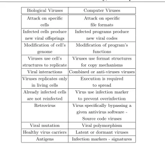
4.2.4 Analogy Between Biological and Computer Viruses . . . 91
4.2.5 Numerical Data and Indices . . . 93
4.2.6 Designing Malware . . . 96
4.3 Non Self-reproducing Malware (Epeian) . . . 98
4.3.1 Logic Bombs . . . 99
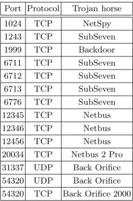
4.3.2 Trojan Horse and Lure Programs . . . 100
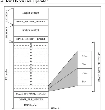
4.4 How Do Viruses Operate? . . . 103
4.4.1 Overwriting Viruses . . . 103
4.4.2 Adding Viral Code: Appenders and Prependers . . . 104
4.4.3 Code Interlacing Infection or Hole Cavity Infection . . . 106
4.4.4 Companion Viruses . . . 110
4.4.5 Source Code Viruses . . . 114
4.4.6 Anti-Antiviral Techniques . . . 117
4.5 Virus and Worms Classification . . . 122
4.5.1 Viruses Nomenclature . . . 122
4.5.2 Worms Nomenclature . . . 141
4.6 Tools in Computer Virology . . . 147
5 Fighting Against Viruses. . . 151
5.1 Introduction . . . 151
5.2 Protecting Against Viral Infections . . . 153
5.2.1 Antiviral Techniques . . . 155
5.2.2 Assessing of the Cost of Viral Attacks . . . 163
5.2.3 Computer “Hygiene Rules” . . . 164
5.2.4 What To Do in Case of a Malware Attack . . . 167
5.2.5 Conclusion . . . 170
5.3 Legal Aspects Inherent to Computer Virology . . . 172
5.3.1 The Current Situation . . . 172
5.3.2 Evolution of The Legal Framework : The Law Dealing With e-Economy . . . 175
Second part - Computer Viruses by Programming 6 Introduction . . . 181
7 Computer Viruses in Interpreted Programming Language 185 7.1 Introduction . . . 185
7.2 Design of a Shell Bash Virus under Linux . . . 186
7.2.1 Fighting Overinfection . . . 188
7.2.2 Anti-antiviral Fighting: Polymorphism . . . 190
7.2.3 Increasing theVbashInfective Power . . . 194
7.2.4 Including a Payload . . . 196
7.3 Some Real-world Examples . . . 197
7.3.1 TheUnix owrVirus . . . 197
7.3.2 TheUnix headVirus . . . 198
7.3.3 TheUnix CocoVirus . . . 199
7.3.4 TheUnix bashvirus . . . 199
7.4 Conclusion . . . 203
Exercises . . . 203
Study Projects . . . 204
APerl Encrypted Virus . . . 204
Disinfection Scripts . . . 205
8 Companion Viruses . . . 207
8.1 Introduction . . . 207
8.2 Thevcomp ex companion virus . . . 210
8.2.2 Weaknesses and Flaws of thevcomp ex virus . . . 219
8.3 Optimized and Stealth Versions of theVcomp exVirus . . . 221
8.3.1 TheVcomp ex v1Variant . . . 221
8.3.2 TheVcomp ex v2Variant . . . 230
8.3.3 Conclusion . . . 238
8.4 TheVcomp ex v3Companion Virus . . . 238
8.5 A Hybrid Companion Virus: theUnix.satyr Virus Case . . . . 241
8.5.1 General Description of theUnix.satyrVirus . . . 241
8.5.2 Detailed Analysis of theUnix.satyr Source Code . . . . 242
8.6 Conclusion . . . 249
Exercises . . . 249
Study Projects . . . 253
Bypassing Integrity Checking . . . 253
Bypassing of theRPM Signature Checking . . . 254
Password Wiretapping . . . 255
9 Worms. . . 257
9.1 Introduction . . . 257
9.2 The Internet Worm . . . 259
9.2.1 The Action of the Internet Worm . . . 260
9.2.2 How the Internet Worm Operated . . . 262
9.2.3 Dealing With the Crisis . . . 265
9.3 IIS Worm Code Analysis . . . 266
9.3.1 Buffer Overflows . . . 267
9.3.2 IISVulnerability and Buffer Overflow . . . 274
9.3.3 Detailed Analysis of the Source Code . . . 274
9.3.4 Conclusion . . . 286
9.4 Xanax Worm Code Source Analysis . . . 286
9.4.1 Main Spreading Mechanisms: Infecting E-mails . . . 287
9.4.2 Executable Files Infection . . . 294
9.4.3 Spreading via the IRC Channels . . . 296
9.4.4 Final Action of the Worm . . . 299
9.4.5 The Various Procedures of the Worm . . . 302
9.4.6 Conclusion . . . 307
9.5 Analysis of the UNIX.LoveLetter Worm . . . 307
9.5.1 Variables and Procedures . . . 308
9.5.2 How the Worm Operates . . . 315
9.6 Conclusion . . . 316
Exercises . . . 317
ApacheWorm Code Analysis . . . 319
Ramen Worm Code Analysis . . . 319
Third Part - Computer Viruses and Applications 10 Introduction . . . 323
11 Computer Viruses and Applications. . . 327
11.1 Introduction . . . 327
11.2 The State of the Art . . . 330
11.2.1 TheXeroxWorm . . . 333
11.2.2 The KOH Virus . . . 335
11.2.3 Military Applications . . . 338
11.3 Fighting against Crime . . . 340
11.4 Environmental Cryptographic Key Generation . . . 342
11.5 Conclusion . . . 347
Exercises . . . 348
12 BIOS Viruses . . . 349
12.1 Introduction . . . 349
12.2bios Structure and Working . . . 351
12.2.1 Disassembly and Analysis of theBIOSCode . . . 352
12.2.2 Detailed Analysis of theBIOS Code . . . 353
12.3vbios Virus Description . . . 357
12.3.1 Viral Boot Sector Concept . . . 358
12.4 Installation of vbios. . . 362
12.5 Future Prospects and Conclusion . . . 364
13 Applied Cryptanalysis of Cipher Systems . . . 367
13.1 Introduction . . . 367
13.2 General Description of Both the Virus and the Attack . . . 369
13.2.1 The VirusV1: the First Infection Level . . . 370
13.2.2 The VirusV2: the Second Infection Level . . . 370
13.2.3 The VirusV2: the Applied Cryptanalysis Step . . . 372
13.3 Detailed Analysis of the ymun20 Virus . . . 373
13.3.1 The Attack Context . . . 373
13.3.2 Theymun20-V1 Virus . . . 375
13.3.3 Theymun20-V2 Virus . . . 377
Study Project . . . 380
Implementing theymun20 Virus . . . 380
Conclusion 14 Conclusion. . . 385
Warning about the CDROM. . . 389
References. . . 391
List of Figures
2.1 Sketch of a Turing Machine . . . 10
2.2 Von Neumann’s Neighborhood . . . 24
2.3 Von Neumann’s Self-reproducing Automata Diagram . . . 30
2.4 Ludwig’s Self-reproducing Automaton . . . 35
3.1 Formal Definition of a Viral Set . . . 45
3.2 Graphical Illustration of the Virus Formal Definition . . . 46
3.3 Flow Model With a Threshold of 1 . . . 58
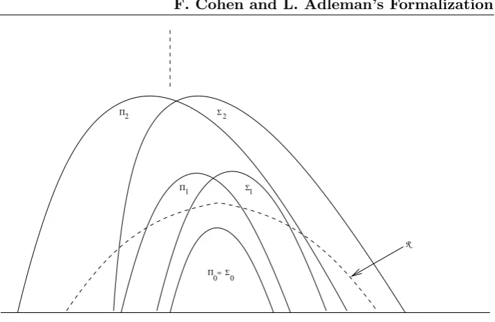
3.4 Πn andΣn Classes and Their Respective Hierarchy . . . 76
4.1 Taxonomy of Malware . . . 82
4.2 Distribution of Malware (January 2002) . . . 94
4.3 Action Mechanisms of a Trojan Horse . . . 101
4.4 Overwriting Mode of Infection . . . 103
4.5 Adding Viral Code: The Appender Case . . . 105
4.6 Structure of aPE Executable File . . . 107
4.7 Infection by Code Interlacing (PE file) . . . 110
4.8 Companion Virus Infection Mode . . . 111
4.9 Source Code Infection . . . 114
4.10 Number of Macro-Virus Alerts (Source: French Civil Service) 127 4.11 Number of Servers Infected by The CodeRed Worm as a Time Function (source [111]) . . . 142
4.13 Distribution of the servers infected by the Sapphire/Slammer Worm (H + 30 minutes). The diameter of each blue circle is relative to the logarithm of the number of locally infected
servers (source: [112]). . . 144
4.14 Evolution of the W32/Bugbear-A worm attack (Oct. 2002 -Source J.-L. Casey) . . . 146
4.15 Evolution dof the W32/Netsky-P and W32/Netsky-PWorms Attacks (July - August 2004) . . . 147
7.1 Vbashp infection . . . 192
8.1 Vcomp ex Virus Infection Principle . . . 211
9.1 Organization of the Example1 Program Stack . . . 271
9.2 IIS Worm Overflow Code Structure . . . 274
9.3 IIS Worm Code Organization . . . 275
9.4 Xanax Worm Paylaod . . . 290
13.1 Functional Flowchart of ymun-V1 Virus . . . 371
13.2 Functional Flowchart of ymun-V2 Virus (Infection Step) . . . 371
13.3 Functional Flowchart of ymun-V2 Virus (Payload) . . . 373
13.4 Infection With ymun20-V1 Virus . . . 376
13.5 ymun20-V1 Virus Action . . . 377
List of Tables
1.1 An Simple Example of Viral Code . . . 4
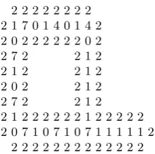
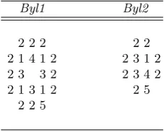
2.1 Turing Machine Computing the Sum of Two Integers . . . 11 2.2 Transition Function Table for Langton’s Self-reproducing Loop 33 2.3 Initial State of Langton’s Self-reproducing Loop . . . 34 2.4 Byl’s Automata Initial States . . . 35 2.5 Byl1 Transition Function Table . . . 36 2.6 Byle2 Transition Function Table . . . 36 4.1 Analogy Between Biological Viruses and Computer Viruses . . 92 4.2 Ports and Protocols Used by the Most Famous Trojan Horses 102 4.3 Formats That May Contain Documents Viruses . . . 126 4.4 Distribution of Main Macro-viruses Types . . . 128
7.1 Source code of thevbash virus . . . 187 7.2 Vbashp virus : restoring function . . . 192 7.3 Vbashp Overinfection Management (MVB first part) . . . 193 7.4 Vbashp Virus: Infection (MVB end) . . . 194 7.5 The Unix owrVirus Source Code . . . 198 7.6 The Unix headVirus . . . 198 7.7 The Unix CocoVirus . . . 200 7.8 The Unix bash(beginning) . . . 201 7.9 The Unix bash(End) . . . 202
1
Introduction
How can we describe what a computer virus really is? What relationship exists between the formal definition of the mathematician1:
∀M ∀V (M, V)∈ V ⇔[V ⊂I∗] et [M ∈ M] et [∀v∈V [∀HM [∀t∀j∈N
[ 1.PM(t) =j et 2. $M(t) = $M(0) et
3. (2M(t, j), . . . ,2M(t, j+|v| −1)) =v]
⇒ [∃v ∈V[∃t, t, j ∈Nett > t
[ 1. [[(j+|v|)≤j] ou [(j+|v|)≤j]]
2. (2M(t, j), . . . ,2M(t, j+|v| −1)) =v et 3. [∃t tel que [t < t< t] et
[PM(t)∈j, . . . , j+|v| −1] ]]]]]]]]
and that of the programmer, given in Table 1.1? Which one is the most convenient to describe what computer viruses really are?
The idea of what a virus is has a different meaning in the non-specialist’s mind, so much so that most of the time viruses are confused with the more general idea of malware (or malicious programs). The term of “virus” for computers appeared only in 1988. However, the artificial beings that are denoted by the term of virus did in fact exist many years before and their theoretical fundaments were established long before their real existence.
for i in *.sh; do
if test ”./$i” != ”$0”; then tail -n 5 $0|cat>>$i ; fi
done
Table 1.1.An Simple Example of Viral Code
A science, a knowledge field, only comes to maturity once formalized. It then allows us to better understand its deep aspects and grasp all the implications. As far as computer virology is concerned, the formalization began seventy years ago with Alan Turing’s works. The works and results of von Neumann, Fred Cohen, Leonard Adleman including those of others which followed, were a pioneering work. They are a solid basic framework for computer virology. These theoretical results are very important both when considering the attacker’s side – viruses and other malware – and the opposite side: defense and antiviral fight. However, this formalization remains far from being achieved.
The formal work of mathematicians during the 1930s largely contributed to the development of viruses. A number of virus writers have discovered a huge field of applications with this formalization. This fact may be less well-known. Early viruses only put von Neumann’s theory of self-reproducing automata into application. In the same way, viral polymorphism did not appear “ex nihilo”. It was directly inspired by the work of von Neumann and Cohen. Many other examples could be given. They prove that the computer viruses that we have to combat today, are, in fact, nothing but the practical applications predicted by long existing theory.
This theoretical formalization helped us model and understand the op-posite face of computer virology, that is to say the antiviral fight. The choice of scanning as the main antiviral technique, since beginning of computer vi-rology, came less from pragmatism than from theoretical considerations and results. These results have also proven the inherent limits of this technique. The same could be said when using with other, more sophisticated antiviral techniques such as integrity checking.
claims of some antiviral softwares publishers. The latter often try to sell us the philosopher’s stone and the squaring of the circle in the same package.
2
The Formalization
Foundations: from Turing to
von Neumann (1936 – 1967)
The art of teaching is made of humility and not pretentiousness: the goal of any lecture is not to make the teacher more intelligent – through a fatuous and uselessly complicated discourse – but to en-able the students to overcome the slightest difficulties and to become more mature-minded.
Emile Gabauriaud-Pag`es
The art of teaching to others (1919)
2.1 Introduction
The formalization of viral mechanisms makes heavy use of the concept of
Turing machines. This is logical since computer viruses are nothing but computer programs with particular functionalities. Formalization of today computer programs began with Alan Turing’s works1 in 1936 [153].
A Turing machine – this definition will be detailed later in this chapter – is the abstract representation of what a computer is and of the programs that may be executed with it. The reader who wishes to learn more deeply on exact relationships between real, everyday life computer and their theoretical model will refer to [26, p. 68]. This theoretical model enables one to solve many essential problems and among them:
1 In fact, a number of important results were obtained during the thirties. Turing’s
• let a function f be given. Is this function really computable ? In other words, does an algorithm exist which can realize, or equivalently compute, the functionf ?
As far as computer viruses are concerned, the function f is the self-reproductionfunction itself. Can a program reproduce? Works of Alan Tur-ing and that of his exegetes did not consider the problem of program self-reproduction.
Only a few years later, the concept of self-reproduction was considered by John von Neumann and Arthur Burks [26, 156] starting from the Tur-ing’s works and results. Their approach was essentially based on cellular automata. In their main result they proved that this property can be prac-tically realized. However, the example they built to prove this result was so complex that researchers since tried to find a less complex example, easier to study and to implement, in order to analyze the self-reproduction feature. The main question that arose at that time was to determine how simple an automaton could be still being able to reproduce.
Next, many authors, particularly Codd [33] in 1968, Herman [89] in 1973, Langton [100] in 1984 and Byl [27] in 1989 managed to build other self-reproducing automata which proved to be far less complex. Self-reproduction then became a practical, operational concept. With it, computer viruses were potentially born but it was only a “first birth”. It was only after still many years that real computer viruses – and the term virus itself – appeared.
2.2 Turing Machines
We are now going to describe precisely what Turing machines are and explore the different problems related to Turing machines, while focusing at the same time on the object of this chapter, that is to say self-reproducing automata. The reader who wishes to have a deeper exposure to Turing machines will refer to [90,101,153]. He will find an interesting and detailed implementation of a Turing machine with theSedinterpreted programming language2in [16, p. 271].
2.2.1 Turing Machines and Recursive Functions
A Turing machine M, a rather primitive system at first sight, is composed of three parts:
• a memory or storage unit which is generally denoted tape. The tape has an infinite length and is divided into cells. Each of the cells contains one symbol at a time, chosen from a given finite set of symbols (thealphabet). A cell is refered as blankwhen it contains no symbol at all. We will con-sider this particular case as the blank symbol, for sake of generalization. There are always a finite number of non blank cells. Initially, the tape contains the input data. At the end of the computation, it contains the output data while during the computation the tape contains temporary data.
• a read/write head which moves left or right on the tape, one cell at a time. The head can read the symbol contained by the current cell or may write a symbol into it. Before any symbol is writtent in a cell, the symbol present in the latter is first erased. Thecurrent cell is the cell in front of which the head is pointing.
• a control function F which drives the read/write head. A memory area which contains the complete state of the machineM and all instructions specific to problems currently processed constitutes the control function. Any move/action of the read/write head is directly determined by both the contents of the memory area and of the current cell. To be more precise, the control function is divided in two other functions3: a state function whose role is to update the internal state of F and a function dedicated to output symbols. The basic operations (or steps) that the read/write head may perform at a rate of one operation per unit time, are:
– moving to the next cell to the right on the tape. – moving to the next cell to the left on the tape.
– not moving. The computation is completed, the machines M halts. – writing a symbol into the current cell.
The work of machine M can thus be summarized by saying that it repeats a certain number of times the three following basics step:
1. Reading step.- The current cell contentxis read and feed to the control function.
3 In fact, the control function is a cellular automaton but this concept will be introduced
Fonction F
Tape
Fig. 2.1.Sketch of a Turing Machine
2. Computing step.- The internal state of the F function is updated as
a function of both its current state and the input valuex.
3. Operation step.- An operation is performed depending on both the
internal state and the input value x.
Despite its apparently primitive aspect, with this very simple model we can express any algorithm and simulate any programming language. Let us now describe what a Turing machine really is, from a theoretical point of vue4.
Definition 1 ATuring machineis a functionM such that for some natural
number n, it is defined by
M :{0,1, . . . , n} × {0,1} → {0,1} × {R, L} × {0,1, . . . , n}
The finite set{0,1, . . . , n}denotes the indices of the machine possible states (or instructions) ei, while the finite set {0,1} describes the two possible
symbolssj that a cell may contain and{R, L}, the set of possible read/write
head movements (to the right or to the left).
Without loss of generality, this definition only considers a very limited set of symbols. However, generalization to larger sets is always possible. In fact, the use of those two symbols is sufficient in itself. Indeed, the input/output tape data format consists of strings of 1’s separated by 0’s. As an example, the integer x is represented by a string of x + 1 symbols 1. To be more precise, the sequence 201 will encoded by 0111010110.
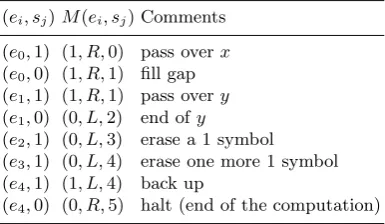
What is the connection between this formal representation and the prac-tical operation of a Turing machine? Let us consider the following example:
4 A number of different ways to formalize Turing machines exist. We considered the most
Table 2.1.Turing Machine Computing the Sum of Two Integers
(ei, sj)M(ei, sj) Comments
(e0,1) (1, R,0) pass overx
(e0,0) (1, R,1) fill gap (e1,1) (1, R,1) pass overy
(e1,0) (0, L,2) end ofy
(e2,1) (0, L,3) erase a 1 symbol
(e3,1) (0, L,4) erase one more 1 symbol
(e4,1) (1, L,4) back up
(e4,0) (0, R,5) halt (end of the computation)
M(4,1) = (0, R,3). This is intended to mean that whenever the machine comes to instruction (state) e4 while scanning a (current) cell in which 1 is written, it is to erase the 1 (leaving a 0 in the cell), move the head just to the right of the current cell and proceed next to instructione3. If the value
M(4,1) is undefined, then whenever the machine comes to instruction e4
while scanning a cell containing a 1, it halts. This the only way to stop a calculation.
Example 1 Let us consider the computation of the sumx+yof two numbers
x and y. The values of machine instructions are listed in Table 2.1. Input data are encoded by
0 111 . . .111 x
0 111 . . .111 y
and the machine starts with the initial statee0 on the leftmost cell containing a 0. At the end of the computation, the tape contains a string (run) ofx+y+1
1’s
This toy example clearly shows how the Turing model is simple and powerful at the same time. As soon as we determine a table which describes the graph of the machine, like in the previous example, then we can compute the relevant operation; in other words we are able to find a feasible solution for the problem we want to solve.
A very essential question is then: is it possible to describe any arbitrary functionf by such a machine? In other words, do problems exist that cannot be described by any Turing machine? To answer to this question we are going to use the concept of recursive functions. Without loss of generality and formalism, we will limit ourself to functions from natural numbers to natural numbers:
which are denotedk-place partial functions (since the definition domain may be only a proper subset of Nk; a function is total if its domain is all ofNk). The input (x1, x2, . . . , xk) of such a function will be encoded in a Turing machine by the following string:
C= 0 11 . . .11 x1+1
0 11 . . .11 x2+1
0. . .11 . . .11 xk+1
0.
Definition 2 A k-place partial function f is said to be recursive if there exists a Turing machine M such that whenever we start M at the initial instruction e0 and scanning the leftmost symbol ofC, then:
1. if f(x1, x2, . . . , xk) is defined, then M eventually halts and the tape
contains the string corresponding to the value f(x1, x2, . . . , xk) (the
read/write head is scanning the leftmost symbol of this string with the tape blank to the right of this string).
2. If f(x1, x2, . . . , xk) is undefined, then M never halts.
Thus, a recursive function is a function which is effectively computable.
The theory of Turing machine and the theory of recursive functions are in fact identical. They are part of the theory of effectively computable func-tions. The reader will refer to [11, 129] for an exhaustive presentation of this theory.
The concept of recursive function was initiated by Kurt G¨odel [85]. The term “recursive”5 was motivated by G¨odel’s concern for a function f to definef(n+ 1) fromf(n). The recursive primitive functions enable to easily enumerate all the recursive functions.
Theorem 1 (Recursive functions cardinality)
There are exactly ℵ0 (a countable infinity of ) partial recursive functions, and there are exactlyℵ0 recursive functions.
Proof. All constant functions are recursive (since they are primitive recursive functions as proven by Church’s Thesis). Hence there at least ℵ06 recursive functions. The G¨odel numbering (see the footnote at the bottom of the
5 Recursiveness is the process by which an object can be defined by another object of
the same essential nature (here the “effectively computable” functions). The class of objects as a whole can be then built in an axiomatic way, that is to say from both a finite number of initial objects and a reduced set of rules. In particular, the class of
primitivefunctions (constant functions, successor function, identity functions...) is the construction basis for all other recursives functions (refer to [129, pp 5-10] for more details).
6 ℵ
Section 2.2.2) shows that there are at most ℵ0 partial recursive functions
hence the results. 2
Theorem 2 (Existence of non recursive functions)
There exists functions which are not recursive.
Proof. By Cantor’s theorem7, there are 2ℵ0 functions (the reader will prove this result as an exercise, by considering the set of functions from Nto the set{0,1}). The theorem follows when considering the Theorem 1. 2
The reader will read [123] to discover some examples of non-recursive func-tions.
Let us add that Definition 2 (as well as the forthcoming results) may generalized in a interesting way tok-ary relations over N, with the following definition.
Definition 3 A relationRis said to be “decidable” if there exists an effec-tive procedure that, given any object x, enables to verify if R(x) is true or not. If R is decidable if and only if its characteristic function is recursive, that is to say effectively computable.
2.2.2 Universal Turing Machine
The model of Turing machines as previously exposed, is not sufficient to describe the behaviour of a real computer. A computer is able to solve a large number of problems while a given Turing machine can only solve with (describe) one problem. In fact, the effective modeling of a true computer requires a more general concept: Univeral Turing Machines(UTM)
Definition 4 A universal Turing machine U is a Turing machine which,
when processing an input, it interprets this input as a description of another given Turing machine, denoted M, concatenated with the description of an input dataxfor that machine. The function ofU is to simulate the behaviour of M processing inputx. We can write U(M;x) =M(x).
In order to better understand this definition, let us explain how a universal Turing machine U really operates. Since a machineM can be described as a finite object, it may be represented (encoded) as an integer8 (a natural number) under some fixed encoding convention. This will enable us to study
7 This theorem asserts that the cardinality of any set is smaller than the cardinality of
the collection of all its subsets.
8 This is very useful “trick,” which has been generalized by G¨odel for the study of first
the way U operates more easily: a machine which is simulating another machine is equivalent to a simple machine processing an input data.
Let us consider a simple example of such an encoding. Let (x0, x1, . . . , xn) be the data written on the tape of a Turing machine. We can represent them as the following integer (G¨odel number):
< x0, x1, . . . , xn>= 2x0+13x1+1. . . px
n+1
n ,
by using – among other solutions – the prime numbers pi (using prime numbers ensures a unique (univocal) decoding by the machine since the fac-torization of any integer into a product of prime numbers is itself unique). Turing machines must be able to perform such an encoding as well as the corresponding decoding process, to operate. More generally, at each time in-stantt, the entire configuration of any machineMitself (the tape’s contents, the instruction number, the cell being scanned) can be described by a finite amount of information, and thus can be encoded into a (G¨odel) number, de-noted theinstantaneous description. The finite set of all the instantaneous descriptions for a machine M – called the computation record or history – can itself be encoded into a natural number (the reader can find a detailed description of this encoding process in [117, §3.1]).
How can we translate the problem of effective computation into the con-text of universal Turing machines? In particular, is the chosen encoding pro-cess itself a recursive function (otherwise considering such encoding would be meaningless)? Knowing the answer is essential in order to be sure that the processing ofU over M with input datax is meaningful. For that purpose, let us consider the following two results.
• There exists a ternary relation R(e, < x0, x1, . . . , xk >, y) which holds if and only if e is a natural number which encodes a Turing machine
M, and y is a computation record for M starting with the input data (x0, x1, . . . , xk) on its tape.
• There exists a recursive function U such that whenever
R(e, < x0, x1, . . . , xk>, y) holds,
then U(y) is the output value of the computation (provided that this value is defined, that is to say that the machine halts).
It is then intuitive enough, in first approach, that relation R is decidable (refer to Definition 3) and that U is recursive. Let us be more precise. Let us consider
ϕe(x0, x1, . . . , xk) =U[y∗]
be thek-place partial function (for any k), where y∗ denotes the smallest y
(when it exists) such that
R(e, < x0, x1, . . . , xk>, y) is true.
Then we can consider the following fundamental theorem from Kleene [95].
Theorem 3 1. The (k+ 1)-place partial function whose value at(e, x0, x1, . . . , xk) isϕe(x0, x1, . . . , xk) is recursive.
2. For each e, the k-place partial function ϕe is recursive.
3. Every k-place recursive partial function equals ϕe for some e.
The number e is called the index of the the function ϕe. Equivalently, a
k-place partial function is recursive – in other words is effectively computa-ble – if and only if it has an index. The notion of index corresponds to the notion of program. In the rest of this part of the book, the notation ϕp will be preferred to the ϕe notation for sake of clarity and the idea of function (simple or universal) will used instead of that of Turing machine. Note that we have just seen that these two concepts are equivalent.
To summarize, a universal function has a program p0 and ϕp0(x) com-putes ϕp(z), where x =< p, z > is the data constitued by a program p and an input data z. Notice that this approach is very powerful, since it no longer allows us to distinguish between data consisting of a program and data consisting of input data. This will prove very useful later on when we consider viruses from a formal point of view.
2.2.3 The Halting Problem and Decidability
The previous formalization, as interesting it may seem, does not solve the problem of whether a prohram halts, that is to say the effective calculability problem. Let us suppose the a machine M receives the dataxas input and starts to compute. After millions of steps, the problem is to determine if the machine will finally halt (and produce a result) or not. One may ask oneself if with thousands of additional steps, the machine will finally halt and give the awaited result.
will decide whether or not this computation ever terminates? Reflecting upon the fact having such a procedure is equivalent to considering another fundamental problem: the decidability or the non-decidability of a function, In other words, we have to consider functions for which there is no program able to calculate them – that is to say these functions are not recursive.
Let us note ϕp(x) if the result of the calculation is undefined and
ϕp(x) if it is defined. Moreover, let us note
H ={p;x|ϕp(x)},
the set of all programs whose computation halts when processing an arbi-trary input datax. We now can give the following fundamental theorem.
Proposition 1 The set H is recursively enumerable.
The expression “recursively enumerable” means that to determine ifp∈H, we start the calculation: if it halts, the membership to the set is de facto
proved, in the contrary no answer can be ever given9. A set which may be defined in such a way – that is to say by means of a program – is said to be recursively enumerable. We now can formulate this property as follows.
Definition 5 A setE is recursive if and only if its characteristic function10 is a total recursive function, that is to say if the program that calculates it
always halts.
A problem whose set of solutions is recursive is called decidable.
It is important to notice that recursive enumerability does not imply the recursive property itself (the reverse is however true). This means that we still do not know if there exists a procedure or an algorithm, which is capable of determining if a computation is effective or not.
Theorem 4 H is not recursive. No program exists that always halts and
gives the result “true” if ϕp(x) or “false” ifϕp(x).
Proof. Let us prove this fundamental theorem by contradiction. Suppose, for the sake of contradiction, that such a program P, exists. It can be used to define, for every programp, a new partial function (or equivalently a new program) Π as follows (we will use in fact its functional representation ψ):
9 The reader will notice that we are here considering an ideal context in which we
dis-carded any time or memory space limitation. However, this does not pose a fundamental problem.
10Thecharacteristic functionof a set is the function defined byf(x) = 1 ifx∈ E and
ψ(p, x) =
if ϕP(< p, x >);
otherwise.
But, by construction,ψ(.) represents the programΠ. How does this program operate when processing a encoded version of itself, that is to say what is the valueψ(Π, Π)? By definition ofψ we have
ψ(Π, Π) =
if ϕP(< Π, Π >);
otherwise.
If ψ(Π, Π) then, by definition, we also have ψ(Π, Π) while if
ψ(Π, Π) , then once again by definition, ψ(Π, Π) . This is a
contra-diction, and hence there can be no such programP.
This fundamental theorem will be used later on by Fred Cohen (refer to Chapter 3) to prove fundamental results on viral detection efficiency.
2.2.4 Recursive Functions and Viruses
The previous results gives us a very powerful model of a computer program. Computer viruses are just instances of computer programs, implementing special functionalities and features (self-reproduction and possibly the abil-ity to evolve), they can thus be described by means of the above results.
The Recursion theorem, due to Kleene [96], and published in 1938, im-plicitly constitutes the very first formalisation – yet unaware – of reproducing programs, many years before von Neumann’s works on self-reproduction (he conducted his earliest works in 1948). The concept of virus will appear much later. With the recursion theorem11, the effectivity (exis-tence) of viral programs is proved.
Theorem 5 (Recursion Theorem) For any total recursive functionf :N→
N, there exists an integer esuch thatϕe(.) =ϕf(e)(.).
This theorem, in a more general form, applies to partial recursive functions as well. To prove this, we just have to use the fact that a total function can be obtained from a partial function (due to theparameter theorem[11, page 544]). The reader will also find an exhaustive presentation of the differents variants of the recursion theorem in [129, pp 180-182]. Since this theorem is very important in the context of viral programs, we give its proof, drawn from Roger’s book [129, p. 180].
Proof. Let any integer ube given. Define a recursive function ψ by:
ψ(x) =
ϕϕu(u)(x) ifϕu(u);
if ϕu(u).
For sake of clarity, the calculation ofψ(x) uses a set of instructions associated (encoded under) the (G¨odel) number u. When u processes itself (that is to say when u processes the input data u; we then consider the formal description of ϕu(u)), if the result, denoted w, is defined, then we use the set of instructions associated to wwith x as input, thus outputing ψ(x), if the latter is defined.
It is obvious that the instructions forψuniformly depend on the number
u. Take g a recursive function which yields, fromu, the G¨odel number for these instructions for ψ. Thus
ϕg(u) =
ϕϕu(u)(x) ifϕu(u);
ifϕu(u).
Now let any recursive functionf be given. Thenf g(the product here means the composition (combination) of functions) is a recursive function. Letvbe a G¨odel number for f g. Sinceϕv =f g is a total function, then ϕv(v) =. Hence, puttingv foru in the definition ofg, we have
ϕg(v)=ϕϕv(v)=ϕf g(v).
Hence the result, sincee=n=g(v) (with the previous index notation;nis
a fixed-point value).
Essentially, the theorem asserts that for a given action (programs performing the same operations), the associated (source) codes themselves are different. If the functionf is the Identity function (f(x) =x, which is a total recursive function, and whose Turing machine is the empty machine), we have source codes which are identical, and hence the implicit notion of self-reproduction, that is to say the concept of simple viruses. For any function f, different from the Identity function, the recursion theorem describes in a very simple and elegant way the mechanism of polymorphism, about fifty years before Cohen’s and Adleman’s works as well as the first practical implementation of a real computer virus. We will see, in the next chapter how L. Adleman classified the different types of malware by using various classes of recursive functions.
source code. This application is better known as “Quine12”. Here is an ex-ample, due to Joe Miller, in the C programming language (the \ symbol does not belong to the original code. We have added it here for sake of pag-ination; the\just indicates that the whole code must be written on a single line):
p="p=%c%s%c;main(){printf(p, 34, p, 34);}"; \ main(){printf(p, 34, p, 34);}
2.3 Self-reproducing Automata
The theory of cellular automata13 was introduced and developed by John von Neumann in 1948. His motivation was to find a reductionist model for biological evolution and more particularly self-reproduction [155].
More precisely, his ambition was to determine a reduced set of primitive local and logical interactions necessary for the evolution of the complex forms of organization essential for life. Following, the cellular automata theory can be defined, from a general point of view, as the study of the problem to determine how complex systems can be generated by a reduced set of simple rules and objects. Cellular automata are the best mathematical model for complex systems and processes that consist of a large number of identical and simple components14, which most of the time interact locally in a non-linearly way.
The cellular automata theory, from work by von Neumann and, later on, Burks [26, 156], quickly went past the mere theoretical fields of both mathematics and computer science and proved itself to be very successful in modeling extremely complex systems in physics, chemistry, biology, bio-chemistry, ecology, economy, military science...
Many different types of cellular automata exist, each of them being tai-lored to fit the requirements of some specific problems and systems. However, all of them possess the following five characterictics:
12The interested reader may consult a very interesting website devoted to Quines,
www.nyx.net/~gthompso/quine.htm, which contains many examples of Quines in many programming languages.
13The termcellularcomes from von Neumann’s publications, in which he considered
two-dimensional space, divided up into square cells, each of them containing a single finite automaton.
14The reader will notice the analogy between cells of a cellular automaton and those of
• A discrete lattice of cells (the word lattice can also be used in its math-ematical sense). The system substrate consists of a one-, two- or three dimensional lattice of identical cells. The number of cells is finite or at least countable.
• Homogeneity: all cells are equivalent.
• Each cell takes on one of a finite number of discrete states.
• Each cell interacts only with cells that are in its local neighborhood (the neighborhood structure depends on the type of cellular automaton).
• At each time instantt, each cell updates its current state according to a transition rule taking into account the state of cells in its neighborhood.
John von Neumann was the first researcher who tried – and succeeded – in building a bidimensional cellular automata, which was able to self-reproduce. In other words, he succeeded in designing what was at the time he lived only a theoretical concept, that is to say a universal Turing machine (or universal computer) [83].
2.3.1 The Mathematical Model of Von Neumann Automata
Definitions
A finite automaton may be defined, in a first approach, as a process able to process initial conditions or data to produce a final result in a finite, countably many or infinite, number of steps. More precisely, the following definition is generally the most widely used.
Definition 6 (Finite automaton)
Formally, a finite automaton is a quintuple (q0, Q, F, X, f). Here Q is a finite set of states where q0 ∈ Q denotes the initial state and F ⊂ Q the set of output (or accepted) states. X is the finite input alphabet while f :
Q×X → Q is the transition. If X∗ denotes the set of all words (strings of any length) defined over alphabet X, then the domain of the function
f extends to Q×X∗ by writing down f(q, m||a) = f(f(q, m), a) for any
m∈X∗, a∈X and q ∈Q. A word m of X∗ is accepted by the automaton if and only if f(q0, m)∈F.
final states. With our notation, for anyn,Q=Vn is called the automaton’s memory.
Bearing the von Neumann’s works and achievements in mind, we will limit ourself to the two-dimensional cellular automata formalisation. The reader will refer to [93] for a more general treatment of general cellular automata (particularly one- or two-dimensional ones). We will rely here on the formalism proposed by J. Thatcher [151].
Let Ndenote the set of natural numbers.
Definition 7 (Cellular automaton)
A cellular automaton (also called cellular space) is defined over N×N by 1. A neighborhood function g:N×N→2N×N defined by
g(α) ={α+δ1, α+δ2, . . . , α+δn} ∀α∈N×N
where + denotes the termwise addition over N×N and the values δi ∈
N×N ,(i= 1,2, . . . , n)are fixed and depend upon the type of automaton.
2. A finite automaton (V, v0, f) where V is the set of cellular states, v0
a distinguished element of V called the quiescent state and f the local transition function from Vn intoV which is subject to the restriction
f(v0, v0, . . . , v0) =v0
A cellular automata can conveniently be seen as a plane assemblage of a countable number of interconnected cells whose cartesian coordinates are contained in the set N×N, with respect to some arbitrarily chosen origin and set of axes. Each cell contains an identical finite automaton (V, v0, f) and the state vt(α) of cell α at time instant t is the state of its associated automaton at that time. Each cell α itself is assumed to be included in the neighborhood ofα, henceδ1= 0.
The neighborhood state functionht:N×N→Vn is defined by
ht(α) = (vt(α), vt(α+δ2), . . . , vt(α+δn)),
and relates the neighborhood state of a cellαat time instanttto the cellular state of that cell at time instantt+ 1 by
f(ht(α)) =vt+1(α).
Definition 8 (Configuration of a cellular automata)
A configuration (or global feasible state of the cellular model) is a function
supp(c) ={α∈N×N|c(α)=v0}
is finite.
A configuration c is a subconfigurationof cif
c|supp(c) =c|supp(c)
where | denotes the functional domain restriction15
By construction, at every time instantt, all cells except a finite number are in the quiesent statev0 (since we have chosen to restrict ourselves to a cellular model in which all cells except a finite number are initially in statev0). The function c is said to have finite support relatively to v0. We notice that it is possible to consider the function c as being equivalent to its functional graph, thus making the use of the term “configuration” appropriate.
Definition 9 (Global transition function)
Let C be the set of all configurations for a given cellular space. Then, the
global transition function F :C → C is defined by
F(c)(α) =f(h(α)) ∀α∈N×N
Given any initial configuration c0, the function F allows us to determine a sequence of configurations (also called a propagation), that is to say a suc-cession of configurations which completely describes the cellular automata evolution (or calculation history):
c0, c1, . . . , ct, . . . withct+1=F(ct) ∀t.
This sequence can also be described by
c0, F(c0), F2(c0), . . . , Ft(c0), . . .
This second notation better describes the automaton’s internal evolution process.
All automaton configurations do not behave in the same way. We will summarize this fact by using the following definition. In what follows, we call an “area” (or zone) any subset U of N×N. An aera thus describes a local restriction of the cellular space itself.
Definition 10 (Configuration properties)
• Two configurations c and c are disjoint if supp(c) ∩supp(c) = ∅. A configuration cand an area U are disjoint if and only if supp(c)∩U =∅.
• Let c and c be disjoint configurations. Their union is defined by
(c∪c)(α) = ⎧ ⎨ ⎩
c(α) if α∈supp(c)
c(α)if α∈supp(c)
v0 otherwise
• A configuration c is calledpassive, if F(c) =cand completely passive if every subconfiguration c of c is passive16
• A configuration cis said to bestable, if there exists a time instant tsuch that Ft(c) is passive.
• A configuration cδ is a translation of configuration c, if there exists an
element δ ∈ N×N such that cδ(α) = c(α −δ) where − denotes the
termwise substraction over N×N.
• Let c and c be two disjoint configurations. We say that configuration c
passes information to configurationc if there exists a time instanttsuch that
Ft(c∪c)|Q=Ft(c)|Q
where
Q=supp(Ft(c)).
Self-reproduction according von Neumann
We now have at our disposal the necessary tools to formally characterize the self-reproduction according to von Neumann’s model. We can now draw a parallel between his cellular automata (also denoted cellular model) and that of Turing machines. The proofs of the results will not be given here since they would need to provide a detailed and tedious description of von Neumann’s cellular automaton. The reader will find them in [151], which is the base of what follows. Let us first make clear that the cellular model which was considered by von Neumann is defined by the following neighborhood17 functiong (see Figure 2.2):
g(α) ={α, α+ (0,1), α+ (0,−1), α+ (1,0)α+ (−1,0)}
16Passivity does not imply complete passivity, by definition of a configuration. The reverse
is however true.
17There exist many other neighborhood functions that are used in various cellular models:
Fig. 2.2.Von Neumann’s Neighborhood
Studying the concept of self-reproduction and more generally of construction requires the ability to determine if a given configuration is obtained or not, after a certain number of steps. It is obvious that the notion of construction only involves the apparition of configurations in areas containing only cells in a quiescent states at the time instantt= 0.
Definition 11 A configurationcconstructsa configurationc if there exists an area U disjoint from configuration c and a time instant t, such that
c =Ft(c)|U.
We now can define self-reproduction in the von Neumann sense.
Definition 12 (Self-reproduction)
A configuration cis said self-reproducingif there exists a translation δ such that c constructs cδ.
Consider the consider the following trivial example drawn from [151].
Example 2 Let be cellular model defined byV ={0,1},v0 = 0 for anyvi :
f(v1, v2, v3, v3, v4, v5) =
1 if v5= 1
v1 if v5= 0
In this model, every configuration is self-reproducing.
On the other hand, self-reproduction is not trivial in von Neumann’s model. In fact von Neumann’s result is extremely impressive when considering his cellular model in detail (see further in Section 2.3.2). The following first result can be given. The reader will find its proof in [151, pp 185-186].
Proposition 2 There exist self-reproducing configurations in von Neumann’s