Article
A PDE-Based Data Reconciliation Approach for
Systems with Variations of Parameters
Siwaporn Duangsri
1,a, Soorathep Kheawhom
2,b, and Pornchai Bumroongsri
1,c,*1 Department of Chemical Engineering, Faculty of Engineering, Mahidol University 2 Department of Chemical Engineering, Faculty of Engineering, Chulalongkorn University E-mail: a[email protected], b[email protected],
c[email protected] (Corresponding author)
Abstract. Data reconciliation is a mathematical approach that improves the quality of measurements by calculating the reconciled data that satisfy the process constraints. The conventional data reconciliation approach relies on the process model that contains the constant parameters. In the industrial applications, however, there are always possible variations of parameters within the system. In this paper, a new data reconciliation approach based on the partial differential equation (PDE) is developed. The proposed data reconciliation approach is experimentally applied to a case study of temperature measurements for a refinery process. The PDE-based model is employed in the formulation of the optimization problem. Unlike the conventional data reconciliation approach in which the system is assumed to be lumped, the PDE-based data reconciliation approach includes in the problem formulation the variations of parameters within the system in order to describe the real system’s behaviour. The reconciled values can be computed within the computational domain so they can be used as the data for troubleshooting, equipment analysis and maintenance.
Keywords: Data reconciliation, partial differential equation, variations of parameters, temperature measurements.
ENGINEERING JOURNAL Volume 23 Issue 4 Received 4 November 2018
1.
Introduction
Chemical processes are usually involved with the technologies that change some reactants into more useful products. In the real operations of chemical processes, the process variables must be measured for monitoring and control at the profitable conditions. The measurement values, however, inevitably contain errors at some certain levels. Thus, a data pre-processing technique is important in the industrial operations. Data reconciliation is one of the techniques extensively used in order to improve the quality of measurements [1-3].
In the conventional data reconciliation approach, the reconciled data can be obtained by solving the optimization problem which minimizes the measurement errors subject to some process constraints [4, 5]. The models based on mass and energy balances are usually employed in order to describe the system behaviour. Plácido et al. [6] applied the data reconciliation approach to a petroleum refinery process in order to detect the unexpected flow deviation and product loss. The quality of the measured data was improved due to the fact that the effects of random and gross errors were reduced. Sarabia et al. [7] applied the data reconciliation approach to the optimal management of hydrogen network in a petrol refinery. The reconciled data strictly satisfied a set of mass balance equations employed in the formulation of the optimization problem. In Nguyen et al. [8], a model of an upstream petroleum plant was developed based on the reconciled data of material and energy streams. The process model employed in the data reconciliation was based on the conservation of mass and energy. In Özyurt and Pike [21], the simultaneous data reconciliation and gross error detection methods were applied to the chemical processes. The quality of the measured data was improved by calculating the reconciled data satisfying the process models. Although the effects of random and gross errors in the measurements are reduced, the conventional data reconciliation approach employs the models with no variations of parameters. For the systems with the variations of parameters, however, a more advanced modeling approach should be developed and included in the formulation of the data reconciliation problem.
Due to some advances in the computational techniques, the partial differential equation (PDE) can be developed to describe the system behaviour within the computational domain. The PDE-based model can be used to predict the values of some variables such as temperature, concentration and so on [9-14] at different positions within the system. Haghshenasfard and Hooman [15] used the PDE to predict the rate of asphaltene deposition from crude oil. It was found that the rate of asphaltene deposition depended on various operating parameters such as temperature, Reynolds number and asphaltene concentration. Bayat et al. [16] predicted the fouling behaviour in an industrial shell and tube heat exchanger. The contours of coke concentration and velocity profile were calculated. Alshammari and Hellgardt [17] performed an analysis for hydrothermal conversion of heavy oil in a continuous flow reactor. The effects of radial mass transport were taken into account using the PDE. The temperature, concentration and velocity profiles in the reactor were computed. Rukthong et al. [18] performed the computational fluid dynamics (CFD) simulation of a pipeline for the crude oil transport. The effects of crude oil properties on the transport profiles were studied.
The variations of parameters usually occur within the system in practice [18-20], e.g., variations of physical and chemical properties within the system. In this paper, the PDE-based model is employed in the formulation of the data reconciliation problem. Unlike the conventional data reconciliation approach [21] in which the models with constant parameters are considered, the PDE-based data reconciliation approach includes in the problem formulation the variations of parameters within the system in order to describe the behaviour of the real system.
The paper is organized as follows. The experimental setup is presented in Section 2. Section 3 describes the modeling equations. The boundary conditions are described in Section 4. The optimization problem formulation is presented in Section 5. The results and discussions are presented in Section 6. Finally, the paper is concluded in Section 7.
2.
Experimental Setup
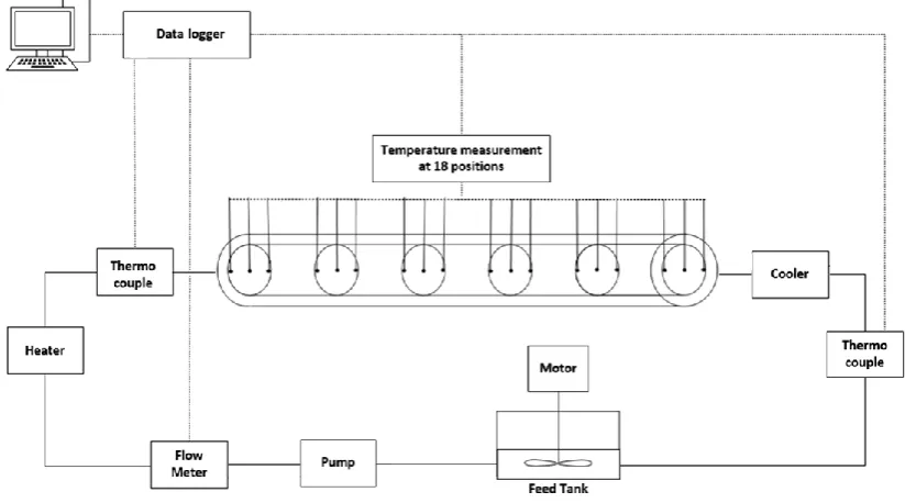
Fig. 1. Flowchart of the experimental setup.
In the experimental setup, the crude oil obtained from an oil refinery in Thailand is contained in a 1 3
m feed tank equipped with a stirrer. The crude oil is supplied to a horizontal pipe for temperature measurements using a feed pump. The pipe length is 3 m and the inner pipe diameter is 0.3 m. At the inlet, the temperature is increased to 330 K using a heater. The values of temperature at 18 measurement positions are measured as shown in Fig. 2.
Fig. 2. Horizontal pipe with 18 measurement positions (PT1-PT18).
[image:3.595.90.502.82.311.2] [image:3.595.87.511.437.630.2]3.
Modeling Equations
The flow is in the turbulent regime. The flow behaviour can be described by the following Reynolds-Averaged Navier-Stokes (RANS) equations [24, 25]
F
)]
)
u
(
u
)(
(
I
[
u
u
u
T Tη
η
p
ρ
t
ρ
(1)0
u
(2)
where is the density,
u
is the velocity vector, p is the pressure, is the dynamic viscosity and F is the body force vector. The turbulent viscosity
T can be calculated from 2
k C
T where k is the
turbulent kinetic energy,
is the turbulent dissipation rate and C 0.09. The k turbulence model can be described by 2 2 1 ) ) u ( u ( u ] ) [( T T k
T k k
t k
ρ (3)
k C k C t ρ T T T 2 2 2 1 2
1
) ) u ( u ( u ] ) [( (4)
where k 1.0, 1.3,C11.44 and C21.92. The values of the model constants are obtained
by comprehensive data fitting for a wide range of turbulent flows [24, 25]. The energy balance consists of the convection and conduction which can be expressed as
)
(
)
u
(
T
T
t
T
C
p
(5)
where Cp is the specific heat capacity, T is the temperature and
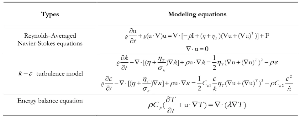
is the coefficient of heatconductivity. The modeling equations can be summarized in Table 1.
Table 1. Modeling equations.
Types Modeling equations
Reynolds-Averaged
Navier-Stokes equations (u )u [ I ( )( u ( u) )] F
u
T T η η p ρ t ρ 0 u
k turbulence model
2 2 1 ) ) u ( u ( u ] ) [( T T k
T k k
t k ρ k C k C t ρ T T T 2 2 2 1 2
1
) ) u ( u ( u ] ) [(
Energy balance equation
(
u
T
)
(
T
)
t
T
C
p
[image:4.595.57.536.555.740.2]The variations of parameters usually occur within the system in practice, e.g., variations of physical and chemical properties within the system. The PDE-based data reconciliation approach includes in the problem formulation the variations of parameters within the system in order to describe the real system’s behaviour. In this paper, the parameters for the flow behaviour and heat transfer as shown in Table 2 are allowed to vary with the temperature [26] at each position within the system.
Table 2. Variations of parameters.
Physical properties Values
Density (kg/m3) ρ8400.59(T20) Specific heat capacity
(J/kg oC)
2 322 0 66875 5 14114
3096 T T
Cp . . .
Dynamic viscosity (Pa.s) 2 3
38 00163 0 38 07271 0 38 36857 1 54674
19. . ( ) . ( ) . ( )
T T T
Coefficient of heat
conductivity (W/m oC) 0.16276(1-0.00054T)
4.
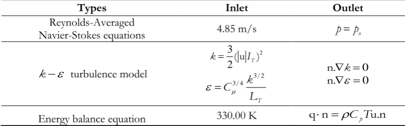
Boundary Conditions
For the Reynolds-Averaged Navier-Stokes (RANS) equations, the velocity is 4.85 m/s at the inlet. At the outlet, a Dirichlet condition on the pressure is specified as
o
p
p (6)
where po is the reference pressure. For the k turbulence model, the values of k and
at the inletcan be calculated from
2
2 3
) u
( IT
k and
T L k C 2 3 4 3 / /
(7)where IT is the turbulence intensity and LT is the turbulent length scale. The value of turbulence
intensity IT is 0.05 for the fully turbulent flow. The turbulent length scale LT is a measure of the size of
eddies that are not solved. For the fully developed flow in pipe, the value of turbulent length scale LT equals
L
07
0. where L is the inner pipe diameter. At the outlet, the following convective flux conditions are
specified for the turbulence variables
0
k
.
n and n. 0 (8)
where
n
is the normal vector. The logarithmic wall function [25] is applied to the wall. For the energy balance equations, the temperature at the inlet is 330 K. At the outlet, the heat flux vector q across the boundary is due to convection asqn
CpTu.n (9) [image:5.595.63.534.179.277.2]Table 3. Boundary conditions.
Types Inlet Outlet
Reynolds-Averaged
Navier-Stokes equations 4.85 m/s p po
k turbulence model
2
2 3
) u ( IT k T L k C 2 3 4 3 / /
0 k . n 0 . nEnergy balance equation 330.00 K qn
CpTu.n5.
Optimization Problem Formulation
In the experiments, the values of temperature are measured at 18 measurement positions as shown in Fig. 2. After the values of temperature have reached the steady state, 100 data sets of the measured temperature
measured ij
T, are collected where the subscript i denotes the measurement position and j denotes the data set.
The objective function of the optimization problem is the following least-squares minimization between the measured temperature Tij,measured and the reconciled temperature Ti,reconciled
minimizing
N i M j i reconciled i d ij,measure T T 1 1 2 ,
(10)
where i is the standard deviation at each measurement position i , N18 is the number of measurement positions and M100 is the number of data sets. The objective function (10) is solved subject to the following constraints; (i) modeling equations in Table 1, (ii) variations of parameters in Table 2, (iii) boundary conditions in Table 3 and (iv) constraints on the minimum and maximum values of the reconciled temperature Ti,reconciled. The PDE-based data reconciliation approach is solved in COMSOL Multiphysics 3.5a
using the optimization module. The details on solving the optimization algorithm can be found in [22, 23]. All of the computations have been performed using Intel Core i3, 2.20 GHz and 4GB RAM.
6.
Results and Discussions
6.1. Mesh Sensitivity Analysis and Model Validation
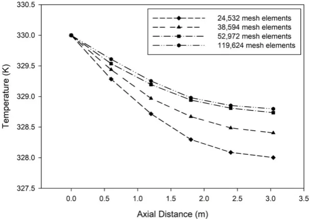
[image:6.595.100.496.105.228.2]Fig. 3. Mesh sensitivity analysis.
Figure 4 shows the simulation temperature at different positions on the centerline. The simulation results are nearly similar as the number of mesh elements is increased from 52,972 to 119,624 so the number of mesh elements 52,972 is selected in this case.
Fig. 4. Simulation temperature at different positions on the centerline.
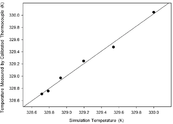
[image:7.595.109.488.78.266.2] [image:7.595.145.449.354.569.2]Fig. 5. Comparison between the simulation temperature and the temperature measured by the calibrated thermocouple.
6.2. PDE-Based Data Reconciliation
In the real industry, the regular thermocouples usually contain the random errors in measurements. Therefore, the proposed data reconciliation approach has been developed to deal with the measurement
errors. In this section, the regular thermocouples with random errors in measurements are used in order to
test the effectiveness of the proposed data reconciliation approach. Figure 6 shows the values of the measured temperature and the reconciled temperature at the inlet (measurement position 2), within the domain (measurement position 8) and at the outlet (measurement position 17). It can be observed that the values of the measured temperature scatter around those of the reconciled temperature due to the effects of random errors.
[image:8.595.157.441.80.284.2]
(c) measurement position 17
Fig. 6. Measured and reconciled temperature at (a) measurement position 2 (b) measurement position 8 and (c) measurement position 17.
Figure 7 shows the averaged values of the measured temperature and the values of the reconciled temperature at different positions on the centerline. The error bars indicate 1.96 standard deviations of the
mean. In contrast to the averaged values of the measured temperature, the PDE-based data reconciliation approach gives the reconciled temperature profile satisfying the PDE-based model.
Fig. 7. Averaged measured temperature and reconciled temperature at different positions on the centerline.
[image:9.595.183.413.75.274.2] [image:9.595.140.454.390.611.2]Fig. 8. Reconciled temperature on the cross-sectional plane at axial position 1.5 m from the inlet.
Figure 9 shows the values of the reconciled temperature on various cross-sectional planes. The temperature profiles on 5 cross-sectional planes are displayed. The proposed data reconciliation approach is based on the PDEs so the values of the reconciled temperature can be computed in axial and radial directions within the computational domain.
Fig. 9. Reconciled temperature on various cross-sectional planes.
[image:10.595.76.519.83.294.2] [image:10.595.68.526.395.601.2]Table 4. Comparison between the PDE-based data reconciliation approach and the conventional data reconciliation approach.
Approaches Reconciled temperature at the inlet (PT2) Reconciled temperature at the outlet (PT17) PDE-based data reconciliation
approach 330.00 K 328.78 K
Conventional data
reconciliation approach [21] 331.05 K 328.45 K
[image:11.595.76.517.118.195.2]The block diagram for the industrial applications of the proposed PDE-based data reconciliation approach is shown in Fig. 10. The proposed data reconciliation approach includes in the problem formulation the variations of parameters within the system in order to describe the real system’s behaviour. The reconciled values can be computed within the computational domain so they can be used as the data in the troubleshooting, equipment analysis and maintenance of the industrial processes. Furthermore, the reconciled values can be used as the data in the process optimization.
Fig. 10. Block diagram for the industrial applications of the proposed PDE-based data reconciliation approach.
[image:11.595.96.504.290.574.2]Fig. 11. Comparison between the reconciled temperature and the temperature measured by the calibrated thermocouple.
7.
Conclusions
In this paper, the PDE-based data reconciliation approach has been developed to improve the quality of the measured data. Unlike the conventional data reconciliation approach in which the system is assumed to be lumped, the PDE-based data reconciliation approach includes in the problem formulation the variations of parameters within the system. The experiment is conducted to demonstrate the implementation of the developed data reconciliation approach. The values of the reconciled temperature can be computed within the computational domain based on the PDE-based model.
Acknowledgements
This research project is supported by Mahidol University, National Research Council of Thailand and Thammasat University through the Research University Network (RUN) Project. The technical supports from the industrial oil refinery in Thailand are gratefully acknowledged.
References
[1] X. Jiang, P. Liu, and Z. Li, “Data reconciliation for steam turbine on-line performance monitoring,” Appl. Therm. Eng., vol. 70, pp. 122-130, 2014.
[2] S. Guo, P. Liu, and Z. Li, “Data reconciliation for the overall thermal system of a steam turbine power plant,” Appl. Energ., vol. 165, pp. 1037-1051, 2016.
[3] S. Srinivasan, J. Billeter, S. Narasimhan, and D. Bonvin, “Data reconciliation for chemical reaction systems using vessel extents and shape constraints,” Comput. Chem. Eng., vol. 101, pp. 44-58, 2017. [4] Z. Zhang, Y. Y. Chuang, and J. Chen, “Methodology of data reconciliation and parameter estimation
for process systems with multi-operating conditions,” Chemometr. Intell. Lab., vol. 137, pp. 110-119. 2014. [5] S. Wu, Q. Ye, C. Chen, and X. Gu, “Research on data reconciliation based on generalized T distribution
with historical data,” Neurocomputing, vol. 175, pp. 808-815, 2016.
[6] J. Plácido, A. A. Campos, and D. F. Monteiro, “Data reconciliation practice at a petroleum refinery company in Brazil,” Comput. Aided Chem. Eng., vol. 27, pp. 777-782, 2009.
[8] T. V. Nguyen, T. Jacyno, P. Breuhaus, M. Voldsund, and B. Elmegaard, “Thermodynamic analysis of an upstream petroleum plant operated on a mature field,” Energy, vol. 68, pp.454-469, 2014.
[9] G. Xu, L. Cai, A. Ullmann, and N. Brauner, “Experiments and simulation of water displacement from lower sections of oil pipelines,” J. Petrol Sci. Eng., vol. 147, pp. 829-842, 2016.
[10] H. Hu and Y. F., Cheng, “Modeling by computational fluid dynamics simulation of pipeline corrosion in CO2-containing oil-water two phase flow,” J. Petrol Sci. Eng., vol. 146, pp. 134-141, 2016.
[11] E. V. P. J. Manjula, W. K. H. Ariyaratne, C. Ratnayake, and M. C. Melaaen, “A review of CFD modeling studies on pneumatic conveying and challenges in modeling offshore drill cuttings transport,” Powder Technol., vol. 305, pp. 782-793, 2017.
[12] K. Kurec, J. Piechna, and K. Gumowski, “Investigations on unsteady flow within a stationary passage of a pressure wave exchanger, by means of PIV measurements and CFD calculations,” Appl. Therm. Eng., vol. 112, pp. 610-620, 2017.
[13] M. Rahimi, S. Movahedirad, and S. Shahhosseini, “CFD study of the flow pattern in an ultrasonic horn reactor: Introducing a realistic vibrating boundary condition,” Ultrason. Sonochem., vol. 35, pp. 359-374, 2017.
[14] C. Zhang, J. Gu, H. Qin, Q. Xu, W. Li, X. Jia, and J. Zhang, “CFD analysis of flow pattern and power consumption for viscous fluids in in-line high shear mixers,” Chem. Eng. Res. Des., vol. 117, pp. 190-204, 2017.
[15] M. Haghshenasfard and K. Hooman, “CFD modeling of asphaltene deposition rate from crude oil,” J. Petrol Sci. Eng., vol. 128, pp. 24-32, 2015.
[16] M. Bayat, J. Aminian, M. Bazmi, S. Shahhosseini, and K. Sharifi, “CFD modeling of fouling in crude oil pre-heaters,” Energ. Convers. Manage., vol. 64, pp. 344-350, 2012.
[17] Y. M. Alshammari and K. Hellgardt, “CFD analysis of hydrothermal conversion of heavy oil in continuous flow reactor,” Chem. Eng. Res. Des., vol. 117, pp. 250-264, 2017.
[18] W. Rukthong, P. Piumsomboon, W. Weerapakkaroon, and B. Chalermsinsuwan, “Computational fluid dynamics simulation of a crude oil transport pipeline: effects of crude oil properties,” Engineering Journal, vol. 20, pp. 145-154, 2016.
[19] E. I. C. Arrieta, C. C. Mancilla, J. Slayton, F. Romero, E. Torres, S. Agudelo, J. Arbeláez, and D. Hincapié, “Experimental investigations and CFD simulations of the blade section pitch angle effect on the performance of a horizontal-axis hydrokinetic turbine,” Engineering Journal, vol. 22, pp. 141-154, 2018.
[20] E. Copertaro, P. Chiariotti, A. A. E. Donoso, N. Paone, B. Peters, and G.M. Revel, “A discrete-continuous method for predicting thermochemical phenomena in a cement kiln and supporting indirect monitoring,” Engineering Journal, vol. 22, pp. 165-183, 2018.
[21] D. B. Özyurt and R. W. Pike, “Theory and practice of simultaneous data reconciliation and gross error detection for chemical processes,” Comput. Chem. Eng., vol. 28, pp. 381-402, 2004.
[22] P. E. Gill, W. Murray, and M. A. Saunders, “SNOPT: An SQP algorithm for large-scale constrained optimization,” SIAM J. Optim., vol. 12, pp. 979-1006, 2002.
[23] Comsol (2012). COMSOL Multiphysics User’s Guide [Online]. Available: http://people.ee.ethz.ch/~fieldcom/pps-comsol/documents/User%20Guide [Accessed: 21 Jan 2018] [24] D. C. Wilcox, “Turbulence energy equation models,” in Turbulence Modeling for CFD, 3rd ed. California:
D.C.W. Industries Inc., 2006. pp. 73-163.
[25] H. K. Versteeg and W. Malalasekera, “Turbulence and its modelling,” in An Introduction to Computational Fluid Dynamics: The Finite Volume Method, 2nd ed. Harlow: Pearson Education Ltd., 2007. pp. 40-113. [26] Z. Guozhong and L. Gang, “Study on the wax deposition of waxy crude in pipelines and its application,”