Computer modelling of the dynamic response of viscoelastic vibroisolators

This is a repository copy of Computer modelling of the dynamic response of viscoelastic vibroisolators.

White Rose Research Online URL for this paper: http://eprints.whiterose.ac.uk/90862/

Version: Accepted Version

Article:

Rongong, J.A. and Kazakoff, A.B. (2006) Computer modelling of the dynamic response of viscoelastic vibroisolators. Engineering Mechanics, 13 (1). 19 - 30. ISSN 1802-1484

[email protected] https://eprints.whiterose.ac.uk/

Reuse

Unless indicated otherwise, fulltext items are protected by copyright with all rights reserved. The copyright exception in section 29 of the Copyright, Designs and Patents Act 1988 allows the making of a single copy solely for the purpose of non-commercial research or private study within the limits of fair dealing. The publisher or other rights-holder may allow further reproduction and re-use of this version - refer to the White Rose Research Online record for this item. Where records identify the publisher as the copyright holder, users can verify any specific terms of use on the publisher’s website.

Takedown

If you consider content in White Rose Research Online to be in breach of UK law, please notify us by

COMPUTER MODELLING OF THE DYNAMIC RESPONSE OF

VISCOELASTIC VIBROISOLATORS

J.A.Rongong*, A.B.Kazakoff**

*Mechanical Engineering, The University of Sheffield, Mappin Street, Sheffield S1 3JD, UK, England.

e-mail: j.a.rongong @shef.ac.uk

**The Institute of Mechanics, Bulgarian Academy of Sciences, Str. “Acad G.Bonchev” block 4., 1113 Sofia, Bulgaria.

e-mail : [email protected]

ABSTRACT: The paper investigates ways to model the response of vibro-isolation mounts that

utilise viscoelastic materials. Simple models based on linear and nonlinear static stiffness are developed. Dynamic response is approximated through appropriate scaling of the viscoelastic Young’s modulus and use of the measured material loss factor. The approach is validated using cylindrical mounts made of polyurethane. The response of a 68 kg mass supported by two mounts and subjected to two different high-amplitude shock loads is predicted. Measured and predicted behaviour correlate closely of the nonlinear model while the linear model gives a reasonable representation. It is noted that the sensitivity of such mounts to temperature is high: the change in response associated with a temperature excursion of 10 °C is significantly greater than the inaccuracy involved with using the linear model.

KEYWORDS: Computer modelling, viscoelastic materials, shock-vibration loading, dynamic

response.

1 INTRODUCTION

Shock mounts made of viscoelastic materials are often used to protect equipment from excessive accelerations. In naval applications for example, viscoelastic mounts support sensitive electronic equipment and their effectiveness in reducing blast-induced acceleration is an important factor in overall warship survivability. The ability to predict the behaviour of shock mounts under high severity shock loads is an important design capability: acceleration levels are needed to specify equipment ruggedness while the displacement envelope defines the sway/rattle spaces needed. There has been significant activity in the naval shock community to develop appropriate modelling methods [1-7]. A series of studies have been carried out to establish guidelines for Finite Element (FE) method for predicting large static [8, 9] and dynamic [1, 5] deformations (up to 70% length change in cylindrical viscoelastic mounts). The disadvantage of FE approach is that it places high demands on computer time and memory. At the early concept design stages, when many different options are being considered, an accurate but numerically more efficient method is needed.

2 MODELLING APPROACH

The simplest model for equipment mounted on a shock-loaded host structure, such as the hull of a ship, is a single degree-of-freedom (SDOF) system subjected to base excitation as shown in Figure 1.

m

)

(x y

c &− & )

(x y

k −

y x

Figure 1: SDOF system with base excitation

The equation of motion is,

0 )

( )

( − + − =

+c x y k x y

x

m&& & & (1)

where the overdot symbol represents time differentiation. Note that the damping and stiffness terms are nonlinear functions of the relative motion between the base and mass respectively. For a given input displacement and velocity history, and , the response of the mass (representing the equipment) can be obtained by direct integration. For such a simple system, the forward difference algorithm is adequate as the time step can be kept very small without incurring significant computational cost. Denoting the relative motion

) (t

y y&(t)

x

y− asX and the time step as h, the response can be obtained using,

n

n t

t ₊₁−

[

]

1

i i

i c X k X

m

x& = & = +

& (2)

where,

1 1

, = ₋ + ₋

−

= _{i i i i i}

i y x x x hx

X& & & & & && (3)

1 1

, = ₋ + ₋

−

= _{i i i i i}

i y x x x hx

X & (4)

Thus the response of the system can be calculated by obtaining appropriate functions for representing stiffness and damping.

3 STIFFNESS AND DAMPING FUNCTIONS

3.1 Nonlinear stiffness function

Homogenous polymeric (viscoelastic) materials normally display near-linear behaviour to large strain levels. Geometric effects however, can create amplitude-dependent nonlinearity. Shock mounts with various different geometries exist. In this paper, a simple mount is used to demonstrate the modelling procedure although same approach may be applied to mounts with more complex shape.

70 mm 70 mm

100 mm viscoelastic

(polyurethane) steel

face plate 10 mm

10 mm steel

face plate

Figure 2: Shock mount configuration and dimensions

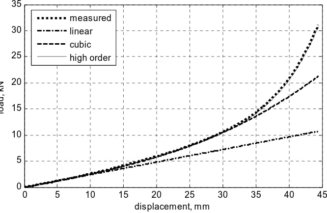
An approximation of the geometric nonlinearity of a mount was obtained by considering its quasi-static stiffness. The load-displacement curve for the mount was obtained by compressing it slowly, to almost one third of its original length, in a hydraulic test machine and is presented in Figure 3. Significant hardening nonlinearity was observed at high deformation.

0 5 10 15 20 25 30 35 40 45

0 5 10 15 20 25 30 35

displacement, mm

lo

ad

, k

N

measured

linear cubic high order

Figure 3: Static compression test – measured and fitted load-displacement behaviour

To match this behaviour, three stiffness functions of differing complexity were fitted to the test data.

X k X

k( )_linear = ₁ (5)

3 3 1

)

(X k X k X

k _cubic = + (6)

7 7 5 5 3 3 1

)

(X k X k X k X k X

k _hiord = + + + (7)

For convenience, the linear coefficient k1 was set as the axial stiffness of a cylinder with fixed ends specified as

(

)

v v v

L S A

E k

2

1

1+β

= , for a cylinder with rigid ends,

v v L r S

2

= (8)

depends on the compressibility of the material in question – for solid, unfilled polymers, it can be assumed that β = 2.

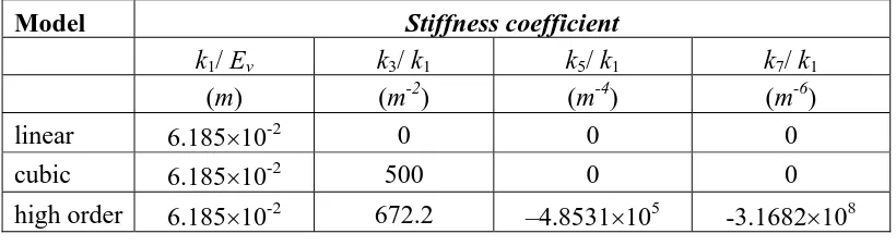
For the polyurethane material used, the static Young’s modulus was taken as 3.9 MPa. The coefficient k1 was obtained from Equation 8 while the higher order coefficients were selected to give the best fit to the measured data and are summarised in Table 1.

Model Stiffness coefficient

k1/ Ev k3/ k1 k5/ k1 k7/ k1

(m) (m-2) (m-4) (m-6)

linear 6.185×10-2 0 0 0

cubic 6.185×10-2 500 0 0

high order 6.185×10-2 672.2 –4.8531×105 -3.1682×108

Table 1: Fitted stiffness coefficients

In Figure 3 it can be seen that the linear model gave a reasonable estimate of stiffness until the deformation reached15mm, the cubic model until 35mm while the high order model worked over the entire range tested. For convenience, it was also assumed that the load displacement curve in tension was similar to the one on compression, thereby allowing characterisation on only one part of the curve. In reality, at large deformations, this would not have been the case because under compression, the free sides of the viscoelastic came into contact with the overhung end caps thereby increasing the stiffness.

3.2 Nonlinear damping function

Energy dissipation in viscoelastic materials is usually characterised and modelled as frequency dependent hysteretic damping rather than viscous. For time-domain response prediction however, it is more convenient to use viscous dampers. One approach is to fit a generalised Maxwell model (i.e. several series spring-dashpot units in parallel) to the material property data. The main challenge with this method is to find suitable coefficients for the individual springs and dampers. A simpler alternate approximation was used in this work. Hysteretic damping was represented using equivalent viscous dampers. The main approximation in this approach is that a characteristic frequency ωc that relates to the response can be specified. For this work, the system was assumed to respond at frequencies close to the linear natural frequency of the SDOF system (i.e.

m k c = 1/

ω ) where m is the mass of the equipment supported by the mount. The damping functions were then,

X k X c c v linear & & ω η ₁ )

( = (9)

3 3

3 1

)

(X k X k X

c

c v

c v

cubic & &

& ω η ω η +

= (10)

7 7 7 5 5 5 3 3 3 1 )

(X k X k X k X k X

c c v c v c v c v

hiord & & & &

& ω η ω η ω η ω η + + +

= (11)

where ηv is the loss factor of the viscoelastic material.

3.3 Temperature and frequency dependence

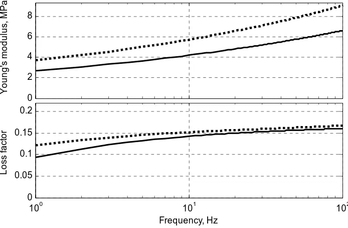
expressions developed (Equations 5-7 and 9-11) the appropriate values of Ev and ηv need to be input. Typically such data is measured at very small strain levels using Dynamic Mechanical Thermal Analysis (DMTA) equipment. For the polyurethane material considered, the effect of temperature and frequency on the Young’s modulus and loss factor are shown in Figure 4.

0 2 4 6 8

Y

o

un

g'

s

m

od

ul

us

,

M

P

a

100 101 102

0 0.05 0.1 0.15 0.2

Frequency, Hz

L

o

ss f

a

ct

o

r

Figure 4: Complex modulus of polyurethane material (solid line, 25°C; dotted line 15°C)

The sensitivity of the material properties can be seen: a 10°C change in temperature (or a decade in frequency) results in a change in modulus of over 50%.

4 INITIAL VALIDATION

A simple experiment was carried out in order to assess the validity of the stiffness and damping scaling suggested. A heavy mass (60 kg) was supported on one mount. The response following a sharp impact from a heavy hammer was measured. The time trace showing decaying vibration amplitude and fitted properties (natural frequency and modal loss factor) is presented in Figure 5.

0 0.2 0.4 0.6 0.8 1 1.2

-2 -1 0 1 2

time, s

a

c

c

e

le

ro

m

e

te

r out

pu

t

v

o

lt

age

natural frequency = 11.8 Hz

modal loss factor = 0.19

Note that the excitation in this case differs from that modelled in Equation 2: for this test, a force was applied directly to the mass and the base was held rigid (i.e. y=0).

While a comparison could have been be achieved by predicting the time response to a suitable shock, the lack of input force measurement (e.g. force transducer on the hammer) made it more convenient to consider the response in the frequency domain. For this initial study, only the cubic system was studied. Also, because it was carried out in the frequency domain, it was possible to use hysteretic damping directly rather than transform it to an equivalent viscous value.

The equation of motion for the undamped cubic system under harmonic excitation is given by,

) sin(

3 3

1X k X F t

k X

m && + + = ω (12)

where m is the mass of the system and F the magnitude of the force. Substituting a trial soution X=X0sin(ωt) and applying a little trignometry gives,

) sin( )} 3 sin( ) sin( { ) sin( )

sin( _{0 3 0}3 ₄3 1₄

0 2 t F t t X k t kX t X

mω ω + ω + ω − ω = ω

− (13)

Retaining only the fundamental components, yields,

F X

k kX X

m + + =

− )

( ₄3 _{3 0}3

0 0 2

ω (14)

The correspondence principle [11] was invoked to replace the real stiffness terms in Equation 14 with complex values to take into account the hysteretic damping in the viscoelastic.

For a shock impact, the force F is not constant with frequency. For an idealised half-sine impact of duration τ (the force history is given by Fpk sin(πt/τ) for 0 ≤ t ≤τ) the force spectrum is give by,

] / [ ) ( ] / [ 2 ) ( 2 ) / ( 1 ) 2 / cos( 2 τ π ω ω τ π ω ω τ π ωτ ωτ πτ = = ≠ = − pk pk F F F F (15)

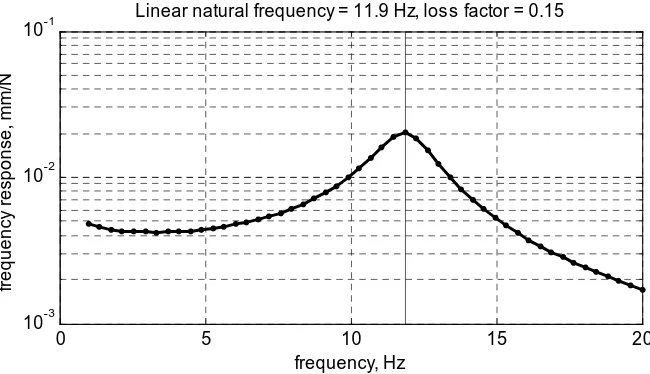
Note that at low frequency, the force spectrum tends towards 2 Fpkτ/πt. Using Equations 14 and 15 in conjunction with the stiffness coefficients (Table 1) and the material data, the response to half-sine shock inputs were calculated. Figure 6 shows the response of the system a 20 °C to a half-sine impact lasting 2.5 ms and reaching a peak vale of 1 kN. It is interesting to observe that at this amplitude the effect of nonlinearity is masked by the relatively high level of damping in the viscoelastic material.

0 5 10 15 20

10-3 10-2 10-1 frequency, Hz fr e q u e n cy re sp o n se , mm/ N

Linear natural frequency = 11.9 Hz, loss factor = 0.15

Figure 6: Predicted frequency response of cubic system to 1 kN peak half-sine shock

loss factor was a little higher than the predicted one (0.19 rather than 0.15). As deformation only occurs in one material the modal loss factor is identical to the material loss factor for the polyurethane. For subsequent calculations, the loss factor of the material was assumed to be 0.19 for the conditions of interest as the impact test was thought to be less prone to error than the DMTA measurement.

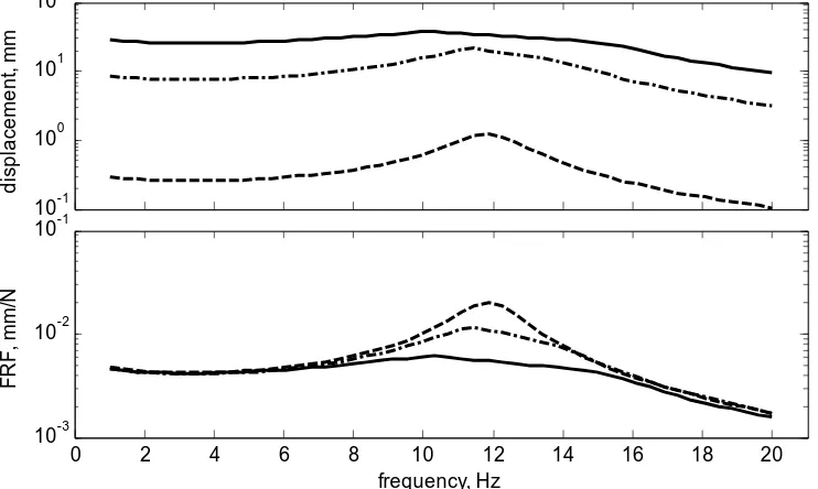
The maximum displacement in the test discussed here was barely visible. The effect of input amplitude on the frequency response was studied using the cubic model – results are presented in Figure 7.

10-1 100 101 102

d

isp

la

ce

me

n

t,

mm

0 2 4 6 8 10 12 14 16 18 20

10-3 10-2 10-1

FR

F,

m

m

/N

frequency, Hz

Figure 7: Effect of shock magnitude on frequency response (dashed line, 1×104 N peak; chain line, 3×105 N peak; solid line, 1×106 N peak;

For half-sine impacts below 10 kN peak, linear and cubic models gave the same response. At higher levels, nonlinear effects stiffening on the FRF) can clearly be seen.

5 VALIDATION OF MODEL FOR LARGE SHOCK INPUTS

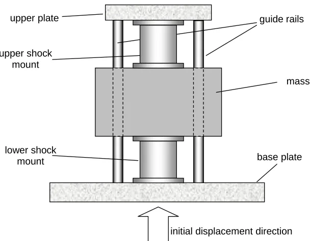
In this section, a comparison is made between the predicted and measured time domain response of a shock mount protected system A sketch of the mount and test rig configuration used for these studies is presented in Figure 8.

base plate guide rails upper plate

mass

initial displacement direction upper shock

mount

lower shock mount

Figure 8: Sketch of shock test arrangement

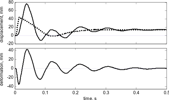
Two shock loading time histories were considered in this study. The measured input (motion at the table, or y in Equation 1) and output (motion of the “equipment” or x in Equation 1) time responses for the first one (named “shot08”), are presented in Figure 9. This figure also shows the deformation seen by the mounts (displayed as x–y in Equation 1).

-20 0 20 40 60 80

d

isp

la

ce

me

n

t,

mm

0 0.1 0.2 0.3 0.4 0.5

-40 -20 0 20 40

de

fo

rm

a

ti

o

n,

m

m

time, s

Figure 9: Measured time histories for shot08 (upper figure: dotted line, input y; solid line, response x)

-20 0 20 40 60 80

d

isp

la

ce

me

n

t,

mm

0 0.1 0.2 0.3 0.4 0.5

-40 -20 0 20 40

de

fo

rm

a

ti

o

n,

m

m

time, s

Figure 10: Measured time histories for shot13 (upper figure: dotted line, input y; solid line, response x)

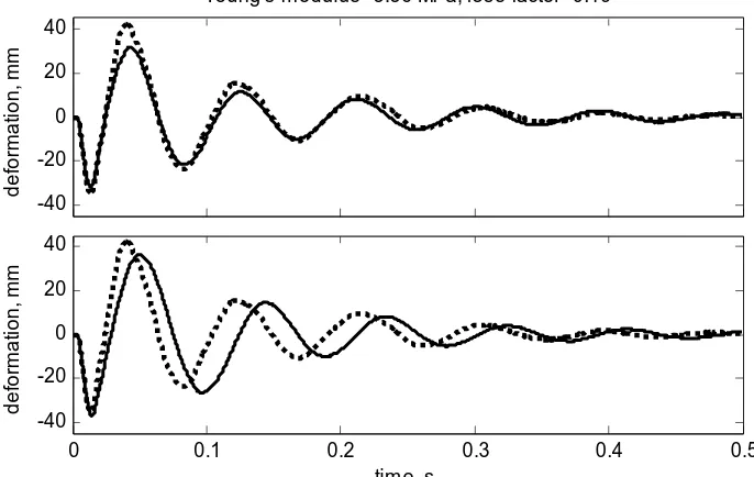
Response predictions were obtained by using the direct integration algorithm described in Equations 2-4. Because of the symmetrical arrangement of the mounts, the stiffness and damping coefficients for the system were simply twice the values found for the coefficients measured in Section 3.

The temperature at which tests were carried out was not measured but was assumed to be 25°C. The characteristic frequency of the system was then given by,

1

2k m

c =

ω (16)

-40 -20 0 20 40

Young's modulus=4.39 MPa, loss factor=0.19

de

for

m

a

ti

on,

m

m

0 0.1 0.2 0.3 0.4 0.5

-40 -20 0 20 40

de

for

m

a

ti

on,

m

m

time, s

Figure 11: Predicted and measured mount deformation history for shot08 (dotted lines, measured x-y; upper figure solid line, predicted x-y using nonlinear model;

lower figure solid line, predicted x-y using linear model)

-40 -20 0 20 40

Young's modulus=3.56 MPa, loss factor=0.19

de

for

m

a

ti

on,

m

m

0 0.1 0.2 0.3 0.4 0.5

-40 -20 0 20 40

de

for

m

a

ti

on,

m

m

time, s

Figure 12: Predicted and measured mount deformation history for shot13 (dotted lines, measured x-y; upper figure solid line, predicted x-y using nonlinear model;

lower figure solid line, predicted x-y using linear model)

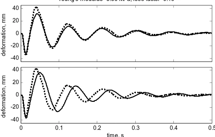
For shot08, there is a close match between predicted and measured responses in both amplitude and frequency. The nonlinear model gave slightly better agreement than the linear one. For the higher amplitude shock (shot13) good agreement is reached for amplitude – although the largest peak (around is underestimated by 15%, the frequency appears to be overestimated. Note that for all the responses calculated, the cubic model gave nominally identical results to the high order one. This is not overly surprising as the deformation remained below 35mm

frequency and manufacturing procedures is well known in viscoelastic polymers: this can easily exceed 20%. Test data for the polyurethane material used here (Figure 4) indicates that this sort of change could be brought about by a 5°C change in temperature. The simulation for shot13 was therefore repeated with the modulus reduced by 20%. Results are presented in Figure 13, where it can be seen that the match for the nonlinear model is very much closer.

-40 -20 0 20 40

Young's modulus=3.56 MPa, loss factor=0.19

de

for

m

a

ti

on,

m

m

0 0.1 0.2 0.3 0.4 0.5

-40 -20 0 20 40

de

for

m

a

ti

on,

m

m

time, s

Figure 13: Predicted and measured mount deformation history for shot13 with reduced E (dotted lines, measured x-y; upper figure solid line, predicted x-y using nonlinear model; lower figure solid line, predicted x-y using linear model)

6 CONCLUSIONS

This work has shown that the transient dynamic response of a mass supported on viscoelastic mounts can be predicted using simple models based on the static load-deflection behaviour of the mounts. For low level shocks a linear model was found to be adequate while for higher levels (up to 60% mount deformation) a cubic model gave good results.

The correct mount stiffness was obtained by scaling the static response by the Young’s modulus ratio between quasi-static and dynamic behaviour at the appropriate temperature and a characteristic frequency (the nominal system resonance frequency).

Nonlinear damping was also modelled using equivalent viscous dampers. The appropriate coefficient was obtained from material properties as the correct temperature and characteristic frequency.

The accuracy of the prediction (in particular, the principal frequency of the response) was found to be sensitive to the environmental conditions to such an extent. The level of uncertainty from this source was found to be more significant that the modelling error.

REFERENCES:

1. G.R.Tomlinson, A.B.Kazakoff and P.R.Thompson, Finite element modeling of viscoelastic elements subjected to large static and dynamic deformations, SAVIAC 69th Shock and Vibration Symposium United Defense, October 12-16, 1998, St.Paul, MN.

3. A.B.Kazakoff, Characterstics of mechanical filters incorporating viscoelastic materials (PART I), Journal of Theoretical and Applied Mechanics, Sofia, 2002, vol. 32, No.4, pp. 11-26

4. A.B.Kazakoff, Characteristics of mechanical filters incorporating viscoelastic materials (PART II), Journal of Theoretical and Applied Mechanics, Sofia, 2003, vol. 33, No.1, pp. 5-20.

5. A.B.Kazakoff, Numerical and experimental investigation on the dynamic response of vibration mounts subjected to large static and dynamic horizontal and vertical deformations. Journal of Theoretical and Applied Mechanics, Sofia, 2003, vol. 33, No. 3, pp. 31-46.

6. Bojcho Marinov, On the Design of Power Transmission Line of a Ship, Archives of Transport, Warsaw, Poland, Vol. 4 (2002), pp. 53-70.

7. L.M. Hadjikov, Al. B. Kazakoff, Ya Ivanov, I. Paskaleva, M. Dashevsky, E. Mironov, Semi-active vibroisolation using elastomer electro-rheological and viscoelastic materials, ECCMR, 2003, 15-17 September 2003, Queen Mary University of London, pp. 411-419.

8. A.B.Kazakoff, S.O.Oyadiji, Finite Element Analysis of Viscoelastic Mounts Subjected to Large Amplitude Half-Sine Loading, The 73-rd Shock and Vibration Symposium, November 18-22, 2002, Newport, Rhode Island, USA.

9. A.B.Kazakoff, S.O.Oyadiji, Experimental Measurement of the Response of Viscoelastic Mounts Subjected to Large Initial Deformation and Half-Sine Shock Impact, The 73rd Shock and Vibration Symposium, November 18-22, 2002, Newport, Rhode Island, USA.