This is a repository copy of
Sociodemographic spatial change in the UK: data and
computational issues and solutions
.
White Rose Research Online URL for this paper:
http://eprints.whiterose.ac.uk/100307/
Version: Published Version
Article:
Norman, PD orcid.org/0000-0002-6211-1625 (2006) Sociodemographic spatial change in
the UK: data and computational issues and solutions. GIS Development - Asia Pacific (10
(12):). pp. 30-34.
[email protected] Reuse
Unless indicated otherwise, fulltext items are protected by copyright with all rights reserved. The copyright exception in section 29 of the Copyright, Designs and Patents Act 1988 allows the making of a single copy solely for the purpose of non-commercial research or private study within the limits of fair dealing. The publisher or other rights-holder may allow further reproduction and re-use of this version - refer to the White Rose Research Online record for this item. Where records identify the publisher as the copyright holder, users can verify any specific terms of use on the publisher’s website.
Takedown
If you consider content in White Rose Research Online to be in breach of UK law, please notify us by
Analysing sociodemographic spatial change in the UK: data and computational
issues and solutions
Paul Norman School of Geography University of Leeds Woodhouse Lane Leeds
LS2 9JT, UK
Tel: (+44) 113 34 38199; Fax: (+44) 113 34 33308
Correspondence to:
Analysing sociodemographic spatial change in the UK: data and computational
issues and solutions
Abstract
In the UK there has been a large expansion in the availability of spatially referenced Census, Vital Statistics and administrative data over the last few decades. This has been paralleled by increases in computer power, the sophistication of analysis packages and of programmer and user skills. To investigate trends and identify change over time we need data consistent in definition over time and space. Unfortunately, a variety of technical issues need to be overcome before even a rudimentary analysis can be carried out.
Attribute data may vary over time in terms of topic availability, definition and the demographic detail for which variables are released. Similarly, the geography for which data are available may change through time either due to a decision about the geographic scale of release or because a boundary change has occurred. These difficulties are compounded by the variety of geographies for which data may be disseminated. For time-series analysis, harmonisation of both attribute and geographical information is essential. In this paper some examples of problems and solutions are given.
Analysing sociodemographic spatial change in the UK: data and computational
issues and solutions
1. Introduction
In the UK there has been a large expansion in the availability of spatially referenced sociodemographic data over the last few decades. This has been paralleled by increases in computer power, the sophistication of analysis packages and of programmer and user skills. The UK’s decennial Census provides detailed sociodemographic information from national to local level. Censuses enable descriptions of population size and characteristics and the calculation of, for example, rates of illness or unemployment by population sub-group and local geographies. We also have high quality information on births and deaths from the Vital Statistics (VS). The VS have been available annually since the 1980s in computerised formats and underpin the calculation of fertility and mortality trends (Rees et al. 2003). We have little information, however, about movements over the life-course due to a paucity of subnational and international migration data since we do not have national registration, unlike Scandinavian countries and the Netherlands.
The application of demographic methods help us study population structure and the components of change. Demographic techniques can reveal inequalities between population sub-groups (by sex, ethnic group or social class, for example) and between locations. To investigate trends and identify change over time we need data consistent in definition over time and space. Unfortunately, there are a variety of issues to be overcome before even a rudimentary analysis can be carried out. Relating to attributes these problems include: changes in the questions asked and the definitions and classifications used and changes in tabulations. In relation to geography, problems include: changes in the scale and type of areas for which data are disseminated and changes in the boundaries of areas for which data are available (Norris and Mounsey 1983).
This paper will first illustrate issues regarding inconsistencies in attribute information over time with some harmonisation solutions identified which researchers might consider using. In the following section, the harmonisation of geographical boundary systems over time is discussed. The overall aim of the paper being to act as a resource for researchers entering this area of research. The issues and techniques being discussed here are being investigated and applied during ongoing demographic research (Norman 2006).
2. Harmonisation of attribute information
have been available annually in computerised formats since 1981 at various geographic scales. Inevitably, an analysis of a sociodemographic time-series will rely on the UK’s decennial censuses which have been collected since 1801 and in computerised formats from 1971. Thus the main focus here is on sources that will help the researcher disentangle inconsistencies in attribute information available in the censuses. Conceptually the challenges of a time-series of births and deaths data are more straightforward but compatibility cannot be assumed.
In terms of continuity between censuses “there is an inherent tension in the decisions over introducing new topics and dropping old ones, reflecting changing needs for information whilst retaining comparability with previous censuses” (Marsh 1993: 7). Thus, the first check to make is whether the topic and questions of interest have been asked in successive censuses. Fortunately, much painstaking work has already been carried out and the researcher should spend time absorbing the wealth of information contained in Norris and Mounsey (1983), Dale (1993) and Champion (1995).
Where the topic exists across time but the detail varies, a researcher might be faced with the following choices: to aggregate differently detailed information to broader groupings that are in common; or to estimate a disaggregation of grouped information to the detail required. The disadvantage of the former is that detail which may have been of interest may be lost, the disadvantage of the latter is that the estimation may be unreliable. Where a topic was not included or information disseminated differently, an estimation using a surrogate variable may be possible. Some examples are outlined below.
It would be reasonable to assume that population counts are consistent from one time point to the next. This will not necessarily be the case since the census population definitional ‘base’ may vary. Dale (1993) identifies two basic methods of enumeration: first, to count everyone present in the household on census night, irrespective of where they usually live; and second, to count everyone who is usually resident in the household, irrespective of whether they are present or absent on census night. Before using population counts as denominators in rates or to calculate change in population size, check that the bases are consistent. Check also whether tables are populations in households or communal establishments and whether students are enumerated at their term-time or parental addresses.
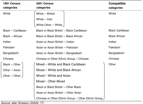
The 8 categories which result (table 1) can be used to investigate changes in ethnic group proportions during the inter-censal period.
[Table 1 about here]
For a longitudinal study 1971-1991, Norman et al. (2005) needed to calculate Carstairs deprivation scores for 1971 but an input variable to this index, Low Social Class, was unavailable for that year. ONS (2004) provide tables linking various socioeconomic classifications. This enabled 1971 Census data on various socioeconomic groups to be approximated as Social Class IV and V using an interim variable NS-SEC Operational Categories (see Table 2).
[Table 2 about here]
The demographic detail in both census and VS data can vary between time points. Census data, for example, tends to be banded into age-groups for confidentiality reasons but this also reduces file sizes that accrue with single year of age information which can prove overwhelming to inexperienced researchers. VS data are also released with age information grouped. Several difficulties with census and VS age information can arise. Age bandings can vary between time points and the detail for which age is released may not be the detail required for a study. Since more demographic detail is released at national and regional levels in census tables than for data released for district and sub-district geographic scales, age bandings can vary between tables from the same census.
A common age banding is for ‘quinary’ 5 year groups. Whilst much sociodemographic data area released for these groupings some variations occur. The oldest age-group has for many years been for those persons aged 85 and over (often labelled 85+). Reflecting increasing life expectancy and ageing populations, more recently quinary data have been released up to ages 85-89 and 90+. The youngest ages often have ages 0 and 1-4 rather than just 0-4 and occasionally there are splits in the late teenage years to allow rates to be appropriate to school age and young adult applications.
To harmonise age bandings, groups can be aggregated to the detail in common between sources. The VS2 has information about the age of mother when she gives birth to a child. Table 3 shows that prior to 2000, the age breakdown in late teenage years is different to that released for 2000 onwards. A solution in this instance is to aggregate to a 16-19 age-group. Alternatively, to match datasets or to have a different grouping from the available information, a disaggregation may be required. Hierarchically applying more detailed information available for a large geographical area to a sub-geography is a strategy worth adopting. For example, if mortality by single year of age were needed for a study at ward level, the grouped information in the VS4 can be disaggregated using national schedules for within group proportions.
The examples given here have flagged difficulties which may be encountered and suggested approaches for harmonising a time-series of attribute data. In the next section of the paper, harmonisation of the geography for which data are released will be considered.
3. Harmonisation of geography
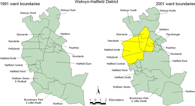
The UK is subject to more administrative boundary changes over time than the rest of Europe put together (ONS, 2000). For example, within local authorities, electoral ward boundaries are regularly adjusted in response to population change to ensure each local authority has similar elector to councillor ratios (Norman et al., 2007). Figure 1 shows that between the 1991 and 2001 Censuses there have been many changes to the constituent wards in the local government district of Welwyn-Hatfield which prevent direct comparisons over time. Even if boundaries do not change, area names and reference codes often vary with different versions and spellings used across years and between different data suppliers and agencies. These issues are compounded by the large number of different geographies for which data are available and by technical difficulties because the UK’s administrative and postal geographies do not align. Unless a consistent geographical approach is taken with time-series data it cannot be known whether changes in the relationships between variables collected for areas are real or an artefact of the boundary system in which they were collected (Norman et al., 2003).
[Figure 1 about here]
A conceptual framework within which to address this problem is a Geographical Conversion Table (GCT) (Simpson 2002a). Essential to a GCT is an estimate of the size of the overlap intersection between source geography (the set of areas in which data pre-exist) and the target geography (the set of zones for which data are needed) so that the data can be apportioned between the boundary systems. ‘Size’ in this application will not be the areal extent but will relate to population distribution since this is not even across space. Thus proxy indicators of distribution are used (Simpson 2002a). Until recently, the tendency has been for ad hoc solutions to particular problems (see Norman et al. 2003; Simpson 2002a); a generically applicable approach is outlined below.
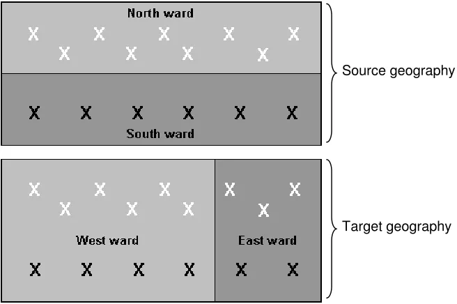
extent as the previous wards and each containing postcodes previously associated with North and South wards.
[Figure 2 about here]
Population data for North ward can be apportioned using the proportion of postcodes falling in the intersection between North and West wards (6/9) and between North and East wards (3/9). Similarly, South ward’s population can be apportioned using the proportion of postcodes in the South and West ward (4/6) and South and East ward (2/6). If the populations of North and South wards were 9,000 and 6,000 these can be apportioned to the alternative wards as follows:
West ward = 10,000 comprising part of North (9,000 x 6/9) plus part of South (6,000 x 4/6) East ward = 5,000 comprising part of North (9,000 x 3/9) plus part of South (6,000 x 2/6)
The assumption of this approach is that the distribution of residential postcodes is a proxy for population distribution. Since people are not evenly distributed across postcodes (with an urban-rural gradient, for example) the disaggregation weights are enhanced by the use of address, person or household counts at each postcode.
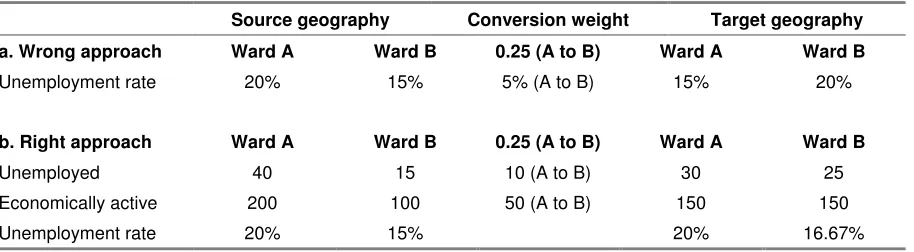
It should be noted that, if sociodemographic data are to be converted from one geography to another, it is the raw counts which must be converted not rates, percentages or other derived data (e.g. deprivation scores or geodemographic profiles). If the unemployment rate for ward ‘A’ was 20% and contiguous ward ‘B’ was 15%, as in table 4, and their shared boundary moved such that a proportion of ward A was transferred to B. 5% unemployment (table 4a) cannot be subtracted from A and added to B. The procedure to adopt is to convert the raw data, then recalculate the rates. Thus, in table 4b, 25% of the numerator and denominator are transferred from ward A to ward B, which does not, in percentage terms result in any change in the unemployment rate in A. The assumption, of course, in this approach is that employed and unemployed persons are similarly distributed at sub-ward level.
[Table 4 about here] 4. Summary
Topical in the UK media are an ageing society, increased life expectancy, low fertility and teenage pregnancy. Immigration is a hot potato during current political debates with large numbers of eastern Europeans, particularly from Poland, moving into the UK following their recent accession into the European Union. There is, however, little acknowledgement of the demographic processes and geographical distributions underlying these phenomena and a danger of reporting without evidence from reliable statistics and independent research. Population geography and demography have the methods, but not always readily usable data, harmonised over time by attribute information and by geographical area, through which to highlight population change, trends and inequalities.
Acknowledgements
• 1991 and 2001 Census statistics have been collected and disseminated by the Office for National
Statistics (ONS) and are Crown Copyright. They are available from ONS and through the Manchester Information and Associated Services (MIMAS), University of Manchester.
• 1991 digital maps are provided by the United Kingdom Boundary Outline and Reference
Database for Education and Research Study (UKBORDERS) via Edinburgh University Data Library (EDINA) with the support of Economic and Social Research Council (ESRC) and the Joint Information Systems Committee of Higher Education Funding Councils (JISC). 1991 boundary material is Copyright of the Crown, the Post Office and the ED-LINE consortium. Digital boundaries for 2001 are provided by ONS and are Crown Copyright.
• Vital Statistics have been made available annually by the Office for Population Censuses and
Surveys (OPCS) and ONS. Prior to 2000, data were obtained from the UK Data Archive, 2000 onwards from ONS. Academic user support for the VS is by ESDS Government http://www.esds.ac.uk/government/ Vital Statistics are Crown Copyright.
• Paul Norman’s research ‘The Micro-Geography of UK Demographic Change: 1991-2001
References
Champion A G (1995) Analysis of change through time. In Census Users’ Handbook (ed. Openshaw S). GeoInformation International: Cambridge: 307-336
Dale A (1993) The content of the 1991 Census: change and continuity. In The 1991 Census User’s Guide (eds. Dale A and Marsh C). HMSO: London: 16-51
Marsh C (1993) An overview. In The 1991 Census User’s Guide (eds. Dale A and Marsh C). HMSO: London: 1-15
Norman P (2006) The Micro-Geography of UK Demographic Change: 1991-2001. Economic and Social Research Council program ‘Understanding Population Trends and Processes’
http://www.geog.leeds.ac.uk/people/p.norman/researchinfo.html
Norman P, Boyle P & Rees P (2005) Selective migration, health and deprivation: a longitudinal analysis. Social Science & Medicine . 60(12): 2755-2771
Norman P, Purdam K, Tajar, A & Simpson S (2007) Representation and local democracy: geographical variations in elector to councillor ratios. Political Geography 26 57-77
Norman P, Rees P and Boyle P (2003) Achieving data compatibility over space and time: creating consistent geographical zones. International Journal of Population Geography 9: 365-386 Norris P & Mounsey H M (1983) Analysing change through time. In A Census User’s Handbook (ed.
D Rhind). Methuen: London: 265-286
ONS (2000) Geography in National Statistics, Office for National Statistics Online: www.statsbase.gov.uk/nsbase/methods_quality/geography/home.aps
ONS (2004) The National Statistics Socio-economic Classification. Online: http://www.statistics.gov.uk/methods_quality/ns_sec/default.asp
Rees P, Brown D, Norman P and Dorling D (2003) Are socioeconomic inequalities in mortality decreasing or increasing within some British regions? An observational study, 1990-98. Journal of Public Health Medicine. 25(3): 208-214
Simpson L (2002a) Geography conversion tables: a framework for conversion of data between geographical units. International Journal of Population Geography 8: 69-82
Table 1: Eight ethnic group categories compatible in both 1991 and 2001 1991 Census categories 2001 Census categories Compatible categories
White White – British White
White – Irish
White Other – White
Black – Caribbean Black or Black British – Black Caribbean Black Caribbean
Black – African Black or Black British – Black African Black African
Indian Asian or Asian British – Indian Indian
Pakistani Asian or Asian British – Pakistani Pakistani
Bangladeshi Asian or Asian British – Bangladeshi Bangladeshi
Chinese Chinese or Other Ethnic Group – Chinese Chinese
Black – Other Mixed – White and Black Caribbean Other
Other – Asian Mixed – White and Black African
Other – Other Mixed – White and Asian
Mixed – Other Mixed
Black or Black British – Other Black
Asian or Asian British – Other Asian
Chinese or Other Ethnic Group – Other Ethnic Group
Source: after Simpson (2002b: 77)
Table 2: Creating a ‘Low Social Class’ variable for 1971
The available data Linking variable The research need
Socioeconomic Group (Table 28, 1971 Census)
Description NS-SEC Operational Categories
NS-SEC Operational Categories
Social Class Description
7 Personal service
workers
12.7, 13.1 IV Partly skilled
occupations
10 Semi-skilled
manual workers
11.2, 12.2, 12.4, 13.2
15 Agricultural workers 12.5, 13.5
11.2, 12.2, 12.4, 12.5, 12.7, 13.1, 13.2, 13.5
11 Unskilled manual
workers
13.4 13.4 V Unskilled
occupations
[image:11.595.72.526.501.654.2]Table 3: Harmonising age detail: aggregation of age of mother at the birth of a child
Data Prior to 2000 Data 2000 onwards Common detail
11-15 11-15 11-15
16 16-17
17-19 18-19 16-19
20-24 20-24 20-24
25-29 25-29 25-29
30-34 30-34 30-34
35-39 35-39 35-39
40-44 40-44 40-44
Age of mother at the
birth of a child
45+ 45+ 45+
Sources: UK Data Archive and ONS
Table 4: Converting rates between geographies
Source geography Conversion weight Target geography
a. Wrong approach Ward A Ward B 0.25 (A to B) Ward A Ward B
Unemployment rate 20% 15% 5% (A to B) 15% 20%
b. Right approach Ward A Ward B 0.25 (A to B) Ward A Ward B
Unemployed 40 15 10 (A to B) 30 25
Economically active 200 100 50 (A to B) 150 150
[image:12.595.71.528.310.436.2]Figure 1: Electoral ward boundary changes 1991 to 2001
Figure 2: Postcodes used to link geographies and weight data conversion
Source: after Norman et al. (2003)
Source geography