Chapter 3
SVM: Support Vector Machines
Hui Xue, Qiang Yang, and Songcan Chen
Contents
3.1 Support Vector Classifier . . . . 37
3.2 SVC with Soft Margin and Optimization . . . . 41
3.3 Kernel Trick . . . . 42
3.4 Theoretical Foundations. . . . 47
3.5 Support Vector Regressor . . . . 50
3.6 Software Implementations. . . . 52
3.7 Current and Future Research . . . . 52
3.7.1 Computational Efficiency . . . . 52
3.7.2 Kernel Selection . . . . 53
3.7.3 Generalization Analysis . . . . 53
3.7.4 Structural SVM Learning . . . . 54
3.8 Exercises . . . . 55
References . . . . 56
Support vector machines (SVMs), including support vector classifier (SVC) and sup-port vector regressor (SVR), are among the most robust and accurate methods in all well-known data mining algorithms. SVMs, which were originally developed by Vapnik in the 1990s [1–11], have a sound theoretical foundation rooted in statisti-cal learning theory, require only as few as a dozen examples for training, and are often insensitive to the number of dimensions. In the past decade, SVMs have been developed at a fast pace both in theory and practice.
3.1
Support Vector Classifier
Optimal Hyperplane wTx+b = 0 x2
x1 r*
r*
[image:2.612.111.338.68.229.2]ρ
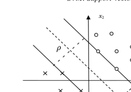
Figure 3.1 Illustration of the optimal hyperplane in SVC for a linearly separable case.
Intuitively, a margin can be defined as the amount of space, or separation, between the two classes as defined by a hyperplane. Geometrically, the margin corresponds to the shortest distance between the closest data points to any point on the hyper-plane. Figure 3.1 illustrates a geometric construction of the corresponding optimal hyperplane under the above conditions for a two-dimensional input space.
Let w and b denote the weight vector and bias in the optimal hyperplane, respec-tively. The corresponding hyperplane can be defined as
wTx+b=0 (3.1)
The desired directionally geometrical distance from the sample x to the optimal hyperplane [12,13] is
r= g(x)
w (3.2)
where g(x)=wTx+b is the discriminant function [7] as defined by the hyperplane
and also called x’s functional margin given w and b.
Consequently, SVC aims to find the parameters w and b for an optimal hyperplane
in order to maximize the margin of separation [ρin Equation (3.5)] that is determined
by the shortest geometrical distances r∗from the two classes, respectively, thus SVC
is also called maximal margin classifier. Now without loss of generality, we fix the functional margin [7] to be equal to 1; that is, given a training set {xi,yi}ni=1 ∈ Rm× {±1}, we have
wTx
i+b≥1 for yi= +1 wTx
i+b≤ −1 for yi = −1
3.1 Support Vector Classifier 39
The particular data points (xi,yi) for which the equalities of the first or second parts in Equation (3.3) are satisfied are called support vectors, which are exactly the closest data points to the optimal hyperplane [13]. Then, the corresponding geometrical
distance from the support vector x∗to the optimal hyperplane is
r∗= g(x
∗)
w = ⎧ ⎪ ⎪ ⎨ ⎪ ⎪ ⎩ 1
w if y ∗ = +1
− 1
w if y ∗= −1
(3.4)
From Figure 3.1, clearly the margin of separationρis
ρ=2r∗ = 2
w (3.5)
To ensure that the maximum margin hyperplane can be found, SVC attempts to
maximizeρwith respect to w and b:
max
w,b 2
w s.t.yiwTxi+b
≥1, i =1, . . . ,n
(3.6)
Equivalently,
min
w,b 1
2w
2
s.t.yi(wTx
i+b)≥1, i =1, . . . ,n
(3.7)
Here, we often use w2 instead ofw for the convenience of carrying out the
subsequent optimization steps.
Generally, we solve the constrained optimization problem in Equation (3.7), known as the primal problem, by using the method of Lagrange multipliers. We construct the following Lagrange function:
L(w,b, α)=1
2w
T
w−
n
i=1
αi yiwTxi+b
−1 (3.8)
whereαiis the Lagrange multiplier with respect to the i th inequality.
Differentiating L(w,b, α) with respect to w and b, and setting the results equal to
zero, we get the following two conditions of optimality:
⎧ ⎪ ⎪ ⎨ ⎪ ⎪ ⎩
∂L(w,b, α) ∂w =0 ∂L(w,b, α)
∂b =0
Then we obtain
⎧ ⎪ ⎪ ⎪ ⎪ ⎪ ⎨ ⎪ ⎪ ⎪ ⎪ ⎪ ⎩
w=
n
i=1 αiyixi
n
i=1
αiyi =0
(3.10)
Substituting Equation (3.10) into the Lagrange function Equation (3.8), we can get the corresponding dual problem:
max
α W (α) = n
i=1 αi−1
2 n
i=1 n
j=1
αiαjyiyjxTi xj
s.t. n
i=1
αiyi =0
αi ≥0, i =1, . . . ,n (3.11)
And at the same time, the Karush-Kuhn-Tucker complementary condition is
αi yiwTxi+b
−1=0, i =1, . . . ,n (3.12)
Consequently, only the support vectors (xi,yi) that are the closest data points to the optimal hyperplane and determine the maximal margin, correspond to the nonzero αis. All the otherαis equal zero.
The dual problem in Equation (3.11) is a typical convex quadratic programming optimization problem. In many cases, it can efficiently converge to the global optimum by adopting some appropriate optimization techniques, such as the sequential minimal optimization (SMO) algorithm [7].
After determining the optimal Lagrange multipliersαi∗, we can compute the optimal
weight vector w∗by Equation (3.10):
w∗= n
i=1 α∗
iyixi (3.13)
Then, taking advantage of a positive support vector xs, the corresponding optimal
bias b∗can be written as [13]:
3.2 SVC with Soft Margin and Optimization 41
3.2
SVC with Soft Margin and Optimization
Maximal margin SVC, including the following SVR, represents the original starting point of the SVM algorithms. However, in many real-world problems, it may be too rigid to require that all points are linearly separable, especially in many complex nonlinear classification cases. When the samples cannot be completely linearly sep-arated, the margins may be negative. In these cases, the feasible region of the primal problem is empty, and thus the corresponding dual problem is an unbounded objective function. This makes it impossible to solve the optimization problem [7].
To solve these inseparable problems, we generally adopt two approaches. The first one is to relax the rigid inequalities in Equation (3.7) and thus lead to so-called soft margin optimization. Another method is to apply the kernel trick to linearize those nonlinear problems. In this section, we first introduce soft margin optimization. Consequently, relative to the soft margin SVC, we usually name SVC derived from the optimization problem [Equation (3.7)] the hard margin SVC.
Imagine the cases where there are a few points of the opposite classes mixed together in the data. These points represent the training error that exists even for the maximum margin hyperplane. The “soft margin” idea aims to extend the SVC algorithm so that the hyperplane allows a few of such noisy data to exist. In particular, a slack
variableξiis introduced to account for the amount of a violation of classification by
the classifier:
min
w,b 1
2w
2+C n
i=1 ξi
s.t. yiwTx i+b
≥1−ξi, ξi ≥0, i =1, . . . ,n (3.15)
where the parameter C controls the trade-off between complexity of the machine and the number of inseparable points. It may be viewed as a “regularization” parameter and selected by the user either experimentally or analytically.
The slack variableξihas a direct geometric explanation through the distance from
a misclassified data instance to the hyperplane. This distance measures the deviation of a sample from the ideal condition of pattern separability. Using the same method of Lagrange multipliers that are introduced in the above section, we can formulate the dual problem of the soft margin as:
max
α W (α)= n
i=1 αi−1
2 n
i=1 n
j=1
αiαjyiyjxiTxj
s.t. n
i=1
αiyi =0
Comparing Equation (3.11) with Equation (3.16), it is noteworthy that the slack
variablesξis do not appear in the dual problem. The major difference between the
linearly inseparable and separable cases is that the constraintαi ≥0 is replaced with
the more stringent constraint 0 ≤ αi ≤ C. Otherwise, the two cases are similar,
including the computations of the optimal values of the weight vector w and bias b, especially the definition of the support vectors [7,13].
The Karush-Kuhn-Tucker complementary condition in the inseparable case is
αi yiwTxi+b
−1+ξi=0, i =1, . . . ,n (3.17)
and
γiξi =0, i=1, . . . ,n (3.18)
whereγis are the Lagrange multipliers corresponding toξithat have been introduced
to enforce the nonnegativity ofξi[13]. At the saddle point at which the derivative of
the Lagrange function for the primal problem with respect toξiis zero, the evaluation
of the derivative yields
αi+γi =C (3.19)
Combining Equations (3.18) and (3.19), we have
ξi =0 if αi <C (3.20)
Consequently, we have the optimal weight w∗as follows:
w∗= n
i=1 α∗
iyixi (3.21)
The optimal bias b∗can be obtained by taking any data point (xi,yi) in the training set for which we have 0< αi∗<C and the correspondingξi=0, and using the data point in Equation (3.17) [13].
3.3
Kernel Trick
3.3 Kernel Trick 43
LetΦ: X→H denote a nonlinear transformation from the input space X⊂Rm to the feature space H where the problem can be linearly separable. We may define the corresponding optimal hyperplane as follows:
wΦTΦ(x)+b=0 (3.22)
Without loss of generality, we set the bias b=0, and simplify Equation (3.22) as:
wΦTΦ(x)=0 (3.23)
Similar to the linear separable cases, we seek the optimal weight vector wΦ∗ in
the feature space in virtue of the similar Lagrange multiplier method, and obtain:
wΦ∗= n
i=1 α∗
iyiΦ(xi) (3.24)
Thus, the optimal hyperplane computed in the feature space is:
n
i=1 α∗
iyiΦ T
(xi)Φ(x)=0 (3.25)
The termΦT
(xi)Φ(x) represents the inner product of two vectors,Φ(x) andΦ(xi). Hence, here we deduce the inner product kernel function:
Definition 3.3.1 (Inner Product Kernel) [7]. Kernel is a function K(x,x), for all x,x ∈X⊂Rm, satisfied:
K(x,x)=ΦT(x)Φ(x) (3.26)
whereΦis a transformation from the input space X to the feature space H.
The significance of the kernel is that we may use it to construct the optimal hy-perplane in the feature space without having to consider the concrete form of the transformationΦ, which usually need not be explicitly formulated in the higher di-mension (even infinite) feature space. As a result, the application of the kernel can make the algorithm insensitive to the dimension, so as to train a linear classifier in a space with higher dimension to solve linearly inseparable problems efficiently. This is done by using K(xi,x) in Equation (3.25) to substituteΦT(xi)Φ(x); then the optimal hyperplane is:
n
i=1 α∗
iyiK(xi,x)=0 (3.27)
However, before implementing the kernel trick, we should consider how to con-struct a kernel function, that is, a kernel function should satisfy which characteristics. To answer this question, we first introduce Mercer’s theorem, which characterizes the
property of a function K(x,x) for when it is considered a true kernel function:
Theorem 3.3.2 Mercer’s Theorem [13] Let K(x,x) be a continuous symmetric kernel that is defined in the closed interval a≤x≤b and likewise for x. The kernel K(x,x) can be expanded in the series
K(x,x)=
∞
i=1
λiϕi(x)ϕi(x) (3.28)
with positive coefficients,λi >0 for all i . For this expansion to be valid and for it to converge, it is necessary and sufficient that the condition
a
b
a
b
K(x,x)ψ(x)ψ(x) dx dx ≥0 (3.29)
holds for allψ(·) for which
a
b
ψ2(x) dx<∞ (3.30)
In light of the theorem, we can summarize the most useful characteristic in the construction of the kernel, which is termed Mercer kernel. That is, for any random limited subsets belonging to the input space X, the corresponding matrix constructed
by the kernel function K(x,x)
K=Kxi,xj
n
i,j=1 (3.31)
is a symmetric and semidefinite matrix, which is called a Gram matrix [7].
Under this requirement, there is still some freedom in how to choose a kernel function in practice. For example, besides linear kernel functions, we can also define polynomial or radial basis kernel functions. More studies in recent years have gone into the research of different kernels for SVC classification and for many other statistical tests. We will mention these in the following section.
3.3 Kernel Trick 45
in practice we often integrate them to exert the different advantages of the two tech-niques and solve the linearly inseparable problems more efficiently. As a result, the corresponding dual form for the constrained optimization problem in the kernel soft margin SVC is as follows:
max
α W (α)= n
i=1 αi−1
2 n
i=1 n
j=1
αiαjyiyjK(xi,xj)
s.t. n
i=1
αiyi =0
0≤αi ≤C, i=1, . . . ,n (3.32) Following the similar Lagrange multipliers method, we can obtain the optimal classifier:
f (x)= n
i=1 α∗
iyiK(xi,x)+b∗ (3.33)
where b∗=1−ni=1α∗iyiK(xi,xs), for a positive support vector ys = +1.
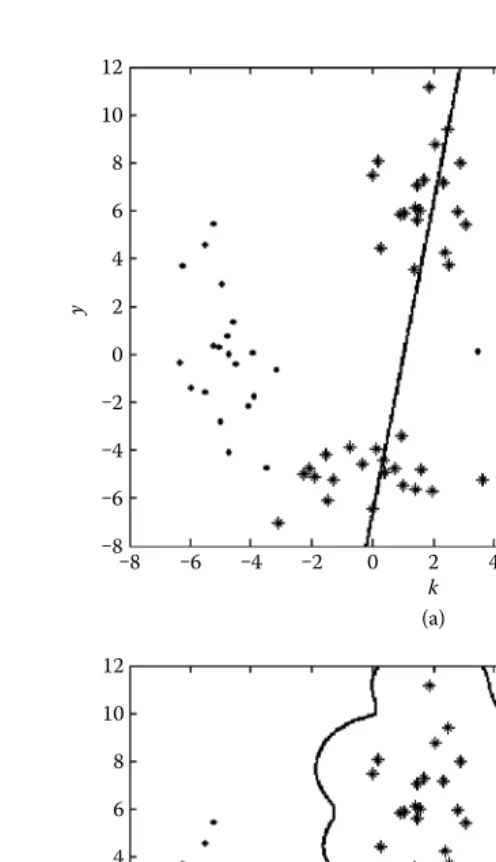
Example 3.3.3 (Illustrative Example) The XOR problem is a typical extremely
linearly inseparabe problem in classification. Here we use it to illustrate the signifi-cance of the soft margin SVC combined with kernel trick in the complex classification problems. A two-dimensional XOR dataset can be randomly generated under four
different Gaussian distributions, where “*” and “•” denote the samples in the two
classes, respectively.
As shown in Figure 3.2a, the hard margin SVC in the linear kernel completely fails in the XOR problem. A linear boundary cannot discriminate the two classes and can be seen to divide all the samples into two parts. This clearly cannot achieve the classification objective for the problem. Consequently, we use the soft margin SVC combined with a radial basis kernel to solve the problem
K(xi,x)=exp
−x−xi2 σ2
We fix the regularization parameter C =1 and the kernel parameter or bandwidth
σ = 1. The corresponding discriminant boundary is presented in Figure 3.2b. By
using the kernel trick, the boundary is no longer linear, for it now encloses only one class. By judging the samples inside or outside the boundary, the classifier can be seen to classify the samples accurately.
Example 3.3.4 Real Application Example SVC algorithm has been widely
12
10 8 6
4 2
0 ‒2
‒4 ‒6 ‒8
‒8 ‒6 ‒4 ‒2 0 2
(a)
4 6 8 10 12
k
y
12
10 8 6
4 2
0 ‒2
‒4 ‒6 ‒8
‒8 ‒6 ‒4 ‒2 0 2
(b)
4 6 8 10 12
k
[image:10.612.103.351.73.504.2]y
3.4 Theoretical Foundations 47
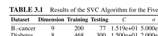
TABLE 3.1
Results of the SVC Algorithm for the Five DatasetsDataset Dimension Training Testing C σ SV Accuracy
B.-cancer 9 200 77 1.519e+01 5.000e+01 138.80 0.7396±4.74
Diabetes 8 468 300 1.500e+01 2.000e+01 308.60 0.7647±1.73
Heart 13 170 100 3.162e+00 1.200e+02 86.00 0.8405±3.26
Thyroid 5 140 75 1.000e+01 3.000e+00 45.80 0.9520±2.19
Splice 60 1000 2175 1.000e+03 7.000e+01 762.40 0.8912±0.66
datasets, respectively, are B.-cancer (breast cancer Wisconsin data), diabetes (Pima Indians diabetes data), heart (heart data), thyroid (thyroid disease data), and splice (splice-junction gene sequences data).
The two to four columns of Table 3.1 summarize some characteristics about the datasets, where Dimension denotes the dimension of the samples, and Training and Testing denote the numbers of the training and testing samples in each dataset. We perform independently repeated 100 runs and 20 runs, respectively, for the first four datasets and splice dataset, which have been offered by the database. Then the av-erage experimental results of the SVC algorithm have been reported in the five to
eight columns of Table 3.1. C andσare the optimal regularization and kernel
param-eters selected by the cross-validation. SV is the average number of support vectors. Accuracy denotes the corresponding classification accuracies and variances.
As shown in Table 3.1, the values of SV are typically less than the numbers of training samples, which validates the good sparsity of the algorithm. Furthermore, the high accuracies show the good classification performance; meanwhile, the relatively low variances show the good stability of SVC in the real applications.
3.4
Theoretical Foundations
In the above sections, we have described the SVC algorithm both in the linearly separable and inseparable cases. The introduction of the kernel trick further improves the expression performance of the classifier, which can keep the inherent linear prop-erty in a high-dimensional feature space and avoid the possible curse of dimension. In this section, we will discuss the theoretical foundation of the SVC. By the Vapnik-Chervonenkis (VC) theory [4,5], we will first present a general error bound of a linear classifier which can guide globally how to control the classifier complexity. We will then deduce a concrete generalization bound of the SVC to explain the significance of the maximum margin in the SVC to guarantee the good generalization capacity of the algorithm.
an analytical generalization bound that can be used for estimating generalization error by defining a new measure of complexity, known as the VC dimension [14,15].
Concretely, assume that training and testing data are generated according to a fixed
but unknown probability distribution D, we define the error errD(h) of a classification
function h on the D as
errD(h)=D{(x,y) : h(x)=y} (3.34)
which measures the expected error [7].
PAC models bound the distribution of the generalization error random variable
errD(hs) and the corresponding PAC bound has the formε =ε(n,H, δ); that is, a
PAC model considers that in the hypothesis hs, the probability of the error in the training data S satisfies [7]:
Dn{S : errD(hs)> ε(n,H, δ)}< δ (3.35)
If there are|H|hypotheses having large errors in the set S, then the PAC bound is
ε=ε(n,H, δ)= 1
n ln
|H|
δ (3.36)
PAC bound presents that the function class H can directly influence the error bound. VC theory further generalizes the PAC bound to the unlimited function class and introduces the concept of the VC dimension d. The VC dimension d measures the maximum number of training data where the function class can still be used to learn perfectly, by obtaining zero error rates on the training data, for any assignment of class labels to these points. Then the generalized PAC bound of a linear classifier can be described as follows:
Theorem 3.4.1 Vapnik and Chervonenkis [7] Let H denote a hypothesis space
whose VC dimension is d. For random probability distribution D on X× {−1,1}, with probability 1−δ, the generalization error of random hypothesis h∈ H on the training set S is no more than
errD(h)≤ε(n,H, δ)=
2 n
log2
δ +d log 2en
d
(3.37)
under the condition that d ≤n, n>2/ε.
In light of the theorem, the first term of Equation (3.37) is the training error, and the second term is proportional to the VC dimension d. Thus, the theorem shows that if we can minimize d, we can minimize the future error, as long as the hypothesis h controls the empirical risk error in a small degree.
3.4 Theoretical Foundations 49
We first give a formal definition of the margin:
Definition 3.4.2 (Margin) [7]. Consider using a real value function class F to classify in the input space X, and the threshold value is 0. We define the margin of
the example (xi,yi)∈X× {−1,1}to the function or hyperplane f ∈F as:
γi =yif (xi) (3.38)
Note thatγi >0 denotes that the example (xi,yi) is correctly classified. The marginal distribution of f corresponding to the training set S is the marginal distribution of the
examples in S. The minimum of the marginal distribution is called the margin mS( f )
of f corresponding to the training set S.
Although the VC dimension d is theoretically meaningful, in practice d is some-times infinite and thus the generalization bound is inapplicable to many real problems. Consequently, we introduce a similar measure related to the margin in SVC instead of the traditional VC dimension:
Definition 3.4.3 (Cover of Function Class) [7]. Let F be a real value function class in X. For a series of input data
S= {x1,x2, . . . ,xn}
Theγ-cover of F is the limited function set B, such that for all f ∈ F , existing
g ∈B, there is max1≤i≤n(|f (xi)−g(xi)|)< γ. N (F,S, γ) denotes the minimal size of the cover. The number of data that Fcovers is
N (F,n, γ)=max
S∈XnN (F,S, γ) (3.39)
Then we use N (F,n, γ) to reformulate Theorem 3.4.1 for the case that the
hypoth-esis f is such that mS( f )=γon the training set S.
Theorem 3.4.4 VC Theorem with Margin [7] Consider a bounded real value
func-tion space F and fixγ ∈R+. For any probability distribution D on X× {−1,1}, with probability 1−δ, the generalization error of a hypothesis f ∈ F on the training set S, which has a margin mS( f )≥γ, satisfies
errD( f )≤ε(n,F, δ, γ)=
2 n
log2
δ +log N (F,2n, γ /2)
(3.40)
under the condition that n>2/ε.
Theorem 3.4.4 shows how to use mS( f ) to bound the generalization error which
can be obtained by the training data. N (F,2n, γ /2) may be viewed as another form
of the VC dimension, where a largerγ corresponds to a smaller N (F,2n, γ /2). As
a result, we may draw a conclusion that large margin can ensure good generalization performance of the classifier for small size samples.
Although Theorem 3.4.4 is a generalization of Theorem 3.4.1, the value N (F,2n,
γ /2) cannot be efficiently quantified in the real-world problems. Consequently, we
Theorem 3.4.5 Generalization Bound of SVC [7] Assume that the input space X is
a hyperball in the inner product space H whose radius is R, X= {x∈H :xH≤ R}.
Consider the function class:
=x→wTx :wH≤1,x∈X
Fixγ ∈R+. For a probability distribution D on X× {−1,1}, with probability 1−δ, the generalization error of a hypothesis f ∈on the training set S, which has the margin mS( f )≥γ, is no more than
errD( f )≤ε(n, , δ, γ)=
2 n
log4
δ +
64R2
γ2 log enγ
4R log
128n R2 γ2
(3.41)
under the condition that n>2/ε, 64R2/γ2<n.
It is noteworthy that the dimension of the input space does not appear in the bound. Hence the bound can be used in the infinite dimension space, which denotes that the bound may overcome the curse of dimension. Furthermore, when the samples distribute well, the bound may guarantee in a high probability that there is a small
error for random testing samples. In that case, the margin γ can be viewed as a
measure about the quality of the sample distribution, and thus may further measure the generalization performance of the SVC algorithm [7].
3.5
Support Vector Regressor
Up to this point, we have focused on the SVC method for classification tasks. In this section, we will consider using SVM to solve nonlinear regression problems, thus called SVR. Similar to the classification algorithm, we also expect to explore the main characteristics of the maximum margin method by exploiting nonlinear functions, which can be obtained using linear learning methods and the kernel trick. In addition, the corresponding algorithms must be efficient under high dimensions [7]. However, for regression problems, the traditional least-squares estimator may not be quite feasible in the presence of outliers, resulting in the regressor to perform poorly when the underlying distribution of the additive noise has a long tail [13]. Thus we need to develop a robust estimator insensitive to small changes in the model; that is, we seek a so-calledε-insensitive loss function.
Definition 3.5.1 (ε-Insensitive Loss Function) [7]
Let f be a real valued function in X. Theε-insensitive loss function Lε(x,y,f ) is
defined as:
3.5 Support Vector Regressor 51
Note that Lε(x,y, f )=0 if the absolute value of the deviation about the estimator output f (x) from the desired response y is less thanεor equal to zero. It is equal to
the absolute value of the deviation minusεotherwise.
Now consider a nonlinear regression model
y=g(x)+v (3.43)
where the additive noise termvis statistically independent of the input vector x. The
function g(·) and the statistics of noisevare unknown. All that we have available is a set of training data
S= {(x1,y1), . . . ,(xn,yn)} and a function class
F = {f (x)=wTx+b,w∈Rm,b∈R}
The objective is to select appropriate parameters w and b, so as to make f (x) approximate the unknown target function g(x). The primal problem can be represented as follows:
min
w,b 1
2w
2 + C n
i=1
(ξi+ξiˆ)
s.t.wTxi+b
−yi≤ε+ξi, i =1, . . . ,n
yi−wTxi+b
≤ε+ξi,ˆ i =1, . . . ,n
ξi,ξiˆ ≥0 i =1, . . . ,n (3.44)
Using the similar method of Lagrange multipliers, the dual problem is:
max
α,αˆ W (α,α)ˆ =
n
i=1
yi( ˆαi−αi) −ε n
i=1
( ˆαi+αi)−1 2
n
i=1 n
j=1
( ˆαi−αi)( ˆαj−αj)xTi xj
s.t. n
i=1
( ˆαi−αi)=0
0≤αi,αiˆ ≤C, i =1, . . . ,n (3.45)
We can further introduce the inner product kernel in the optimization problem Equation (3.45), and extend the regression algorithm to a feature space so as to make the nonlinear functions able to be obtained by means of the linear learning machines in the kernel space.
Compared with SVC, SVR has an additional free parameterε. The two free
pa-rametersεand C control the VC dimension of the approximating function
f (x)=wTx= n
i=1
( ˆαi−αi)K(xi,x) (3.46)
when we set the bias b = 0.ε and C should be selected by the user and directly
influence the complexity control for regression. How to selectεand C simultaneously
3.6
Software Implementations
LibSVM [16] and SVMlight [17] are two of the most famous software about the implementation of SVM algorithms.
LibSVM provides not only compiler languages used in the Windows system, but also C++ and Java source codes which are easy to improve, revise, and apply in other operating systems. Specially, LibSVM has relatively fewer tunable parame-ters involved in SVM algorithms than other software and provides lots of default parameters to solve real application problems effectively.
SVMlight is another implementation in C language. It adopts an efficient set se-lection technique based on steepest feasible descent, and two effective computational policies “Shrinking” and “Caching” of kernel evaluations. SVMlight mainly includes two C programs: SVM learn, used for learning training samples and training the cor-responding classifier, and SVM classifiy, used for classifying testing samples. The software also provides two efficient estimation methods for assessing the general-ization performance: XiAlpha-estimates, computed at essentially no computational expense but conservatively biased, and Leave-one-out testing, almost unbiased.
Furthermore, there are lots of complete machine learning toolboxes, including
SVM algorithms, such as Torch (in C++), Spider (in MATLAB), and Weka (in Java),
which are all available at http://www.kernel-machines.org.
3.7
Current and Future Research
In the past decade, SVMs have been developed at a fast pace both in theory and in practice. Many future works remain. In this section, we enumerate a few of the major research directions where major progress is being made and many research problems are still open.
3.7.1
Computational Efficiency
One of the initial drawbacks of the SVMs is its costly computational complexity in the training phase, which leads to inapplicable algorithms in the large datasets. However, this problem is being solved with great success. One approach is to break a large optimization problem into a series of smaller problems, where each problem only involves a couple of carefully chosen variables so that the optimization can be done efficiently. The process iterates until all the decomposed optimization problems are solved successfully.
3.7 Current and Future Research 53
learning problems on these core sets can produce good approximation solutions in very fast speed. For example, the core vector machine [18] and the further ball vector machine [21] can learn SVMs for millions of data in seconds.
3.7.2
Kernel Selection
In the kernel SVMs, the selection of the kernel function is generally required to satisfy the Mercer’s theorem. Hence, the common kernel functions involve three types, that is, sigmoid, polynomial, and radial basis functions, which may sometimes limit the applicability of the kernel trick. Recently, Pekalska et al. provided a novel view to design a kernel function based on a general proximity relation mapping [22]. The new kernel function needs neither be satisfied by the Mercer’s conditions nor be limited to only one feature space, and shows better classification performance than the common Mercer kernels experimentally. However, the theoretical foundation of the new generalized kernel needs further research.
Furthermore, another popular approach is multiple kernel learning which consid-ers more than one kernel; through the combinations one can achieve better results [23–29]. This is similar to using an ensemble of kernels. By setting the proper objec-tive functions, better selection of the kernel parameters can be done to allow mixture kernels.
3.7.3
Generalization Analysis
We are accustomed to using the VC dimension to estimate the generalization er-ror bound of the kernel machines. However, the bound involves a fixed complexity penalty which does not depend on the training data, which as a result, cannot be made universally effective [30]. To solve this problem, Rademacher’s complexity is introduced as an alternative to evaluate the complexity of a classifier instead of the classical VC dimension [31–34], which is based on the intuition that we can measure the capacity (or complexity) of a classifier by its ability to fit random data. It is defined as follows:
Definition 3.7.1 (Rademacher Complexity) [35]. For the sample S =
{x1, . . . ,xn}generated by a distribution D on a set X and a real value function class F with domain X, the empirical Rademacher complexity of F is the random variable
ˆRn(F)=E
sup f∈F
2 n n
i=1 σif (xi)
x1, . . . ,xn
(3.47)
where= {σ1, . . . , σn}are independent uniform{±1}-valued (Rademacher) random
variables. The Rademacher complexity of F is
Rn(F)=ES[ ˆRn(F)]=ES
sup f∈F
2 n n
i=1 σif (xi)
The sup part inside the expectation formula measures the best correlation that can be found between a function of the class and the random labels. Furthermore, in the kernel machines, we can obtain an upper bound to the Rademacher complexity:
Theorem 3.7.2 Complexity Analysis [35]. If k : X×X → R is a kernel, and S = {x1, . . . ,xn} is a sample of points from X, then the empirical Rademacher complexity of the classifier FBsatisfies
ˆRn(FB)≤ 2B n
n
i=1
k(xi,xi)= 2B n
tr (K) (3.49)
where B is the bound of the weights w in the classifier.
It is noteworthy that the bound of the Rademacher complexity only involves the trace of the corresponding kernel matrix, which is determined by the concrete training data. It is more feasible to use than the traditional VC dimension to control the complexity of a classifier as well as estimate the generalization performance.
3.7.4
Structural SVM Learning
Margin maximization is the initial motivation of the SVM algorithms [36]. Con-sequently, SVM (SVC) usually places more focus on the separability between the classes of samples but does not sufficiently use the prior data distribution information within classes. The well-known “No Free Lunch” theorem [12] indicates that there does not exist a pattern classification method that is inherently superior to any other, or even to random guessing without using additional information. It is the type of problem, prior information, and the amount of training samples that determine the form of classifier to apply. In fact, corresponding to different real-world problems, different classes may have different underlying data structures. A classifier should ad-just the discriminant boundaries to fit the structures which are vital for classification, especially for the generalization capacity of the classifier. However, the traditional SVM does not differentiate the structures, and the derived decision hyperplane lies unbiasedly right in the middle of the support vectors [36,37], which may lead to a nonoptimal classifier in the real-world problems.
3.8 Exercises 55
The second approach is by exploiting clustering algorithms [40] by assuming that the data contain several clusters that hold the prior distribution information. This assumption seems more general than the manifold assumption, which has in fact led to several popular large margin machines. A recent approach is known as structured large margin machine (SLMM) [37]. SLMM applies clustering techniques to capture the structural information in the different classes first. It then uses the Mahalanobis distance as a distance measure from the samples to the decision hyperplanes, instead of the traditional Euclidean distance, to introduce the involved structure information into the constraints. Some popular large margin machines, such as support vector machine minimax probability machine (MPM) [41], and maxi-min margin machine
(M4) [36], can all be viewed as the special cases of SLMM. Experimentally, SLMM
has shown better classification performance. However, since the optimization problem of SLMM is formulated as sequential second order cone programming (SOCP) rather than the QP in SVM, SLMM has much higher computational cost in training time as compared to traditional SVM. Furthermore, it is not easy to be generalized to large-scale or multiclass problems. Consequently, a novel structural support vector machine (SSVM) was developed in [42] to exploit the classical framework of SVM rather than as constraints in SLMM. As a result, the corresponding optimization problem can still be solved by the QP as in SVM, and keep the solution not only sparsity but also scalability. Furthermore, SSVM has been shown to be theoretically and empirically better in generalization than SVM and SLMM.
3.8
Exercises
1. Consider a simple binary classification problem:
c1: (1,1)T (−1,3)T (2,6)T c2: (−1,−2)T (1,−3)T (−5,−7)T (a) Compute the optimal hyperplane and geometrical margin. (b) Point out the support vectors.
(c) Using the method of Lagrange multipliers, compute the solution in the dual space.
2. Consider another binary classification problem:
c1 : (1,1)T (3,7)T (5,9)T c2 : (−1,−2)T (1,6)T (2,−1)T
Use a soft margin SVC to construct the optimal hyperplane and compute the corresponding solution in the dual space.
4. Let K1and K2be the kernels in X×X, X⊆Rn, a∈R+, f (·) be a real value function in X:
φ: X→Rm
where K3is a kernel in Rm×Rm, and B is an n×n symmetrical semidefinite
matrix. Prove the following functions are kernel functions:
(a) K(x,z)=K1(x,z)+K2(x,z)
(b) K(x,z)=aK1(x,z)
(c) K1(x,z)K2(x,z)
(d) K(x,z)= f (x) f (z)
(e) K(x,z)=K3(φ(x), φ(z))
(f) K(x,z)=xTBz
5. Discuss the generalization bounds of SVR derived from the VC theorem. 6. We have discussed the use of SVC for binary classification problems. Discuss
how to extend SVC to solve multiclass classification problems. 7. Discuss the robustness properties of SVM algorithms.
8. Discuss the cases that SVC does not sufficiently use the prior data distribution information within classes, where the resulting discriminant hyperplane lies right in the middle of the support vectors.
References
[1] V. Vapnik. The Nature of Statistical Learning Theory, Springer Verlag, 1995.
[2] V. Vapnik. Statistical Learning Theory, Wiley, 1998.
[3] B. Sch¨olkopf, C.J.C. Burges, and A.J. Smola. Advances in Kernel Methods—
Support Vector Learning, MIT Press, 1999.
[4] O. Chapelle, P. Haffner, and V. Vapnik. Support vector machines for
histogram-based image classification. IEEE Trans. on Neural Networks, vol. 10(3.5), 1055–1064, 1999.
[5] C. Cortes and V. Vapnik. Support vector networks. Machine Learning, vol. 20,
273–297, 1995.
[6] N. Cristianini, C. Campbell, and J. Shawe-Taylor. A multiplicative updating
algorithm for training support vector machine. In Proceedings of the 6th Euro-pean Symposium on Artificial Neural Networks (ESANN), 1999.
[7] N. Cristianini and J. Shawe-Taylor. An Introduction to Support Vector Machines
References 57
[8] M.S. Kearns, S.A. Solla, and D.A. Cohn. Advances in Neural Information
Processing Systems, MIT Press, 1999.
[9] U.M. Fayyad, G. Piatetsky-Shapiro, P. Smythand, and R. Uthurusamy.
Ad-vances in Knowledge Discovery and Data Mining, MIT Press, 1996.
[10] A.J. Smola, P. Bartlett, B. Sch¨olkopf, and C. Schuurmans. Advances in Large
Margin Classifiers, MIT Press, 1999.
[11] B. Sch¨olkopf. Support Vector Learning, R. Oldenbourg Verlag, 1997.
[12] R.O. Duda, P.E. Hart, and D.G. Stork. Pattern Classification, Wiley, 2001.
[13] S. Haykin. Neural Networks: A Comprehensive Foundation, Tsinghua
Univer-sity Press, 2001.
[14] V. Cherkassky, X. Shao, F. Mulier, and V. Vapnik. Model complexity control
for regression using VC generalization bounds. IEEE Transactions on Neural Networks, vol. 10, 1075–1089, 1999.
[15] V. Cherkassky and F. Mulier. Learning From Data: Concepts, Theory and
Methods, Wiley, 1998.
[16] C.-C. Chang and C.-J. Lin. LibSVM: A library for support vector machines.
Software available at http://www.csie.ntu.edu.tw/∼cjlin/libsvm, 2001.
[17] T. Joachims. Making Large-scale SVM learning practical. Advances in Kernel
Methods—Support Vector Learning, B. Sch¨olkopf, C. Burges, and A. Smola (eds.), MIT Press, 1999.
[18] I. W. Tsang, J.T. Kwok, and P.-M. Cheung. Core vector machines: Fast SVM
training on very large data sets. Journal of Machine Learning Research, vol. 6, 363–392, 2005.
[19] I.W. Tsang, J.T. Kwok, and K.T. Lai. Core vector regression for very large
regression problems. ICML, 913–920, 2005.
[20] I.W. Tsang and J.T. Kwok. Large-scale sparsified manifold regularization.
NIPS, Vancouver, Canada, 2006.
[21] I.W. Tsang, A. Kocsor, and J.T. Kwok. Simpler core vector machines with
enclosing balls. ICML, 2007.
[22] E. Pekalska, P. Paclik, and R.P.W. Duin. A generalized kernel approach
to dissimilarity-based classification. Journal of Machine Learning Research, vol. 2, 175–211, 2001.
[23] J. Bi, T. Zhang, and K. Bennett. Column-generation boosting methods for
mixture of kernels. KDD, 521–526, 2004.
[24] I.M. de Diego, J.M. Moguerza, and A. Munoz. Combining kernel information
for support vector classification. Multiple Classifier Systems, 102–111, 2004.
[25] Y. Grandvalet and S. Canu. Adaptive scaling for feature selection in SVMs.
[26] G.R.G. Lanckriet, T.D. Bie, N. Cristianini, M.I. Jordan, and W.S. Noble. A statistical framework for genomic data fusion. Bioinformatics, vol. 20(3.16), 2626–2635, 2004.
[27] G.R.G. Lanckriet, N. Cristianini, P. Bartlett, L.E. Ghaoui, and M.I. Jordan.
Learning the kernel matrix with semidefinite programming. JMLR, vol. 5, 27– 72, 2004.
[28] C.S. Ong, A.J. Smola, and R.C. Williamson. Learning the kernel with
hyper-kernels. JMLR, vol. 6, 1043–1071, 2005.
[29] Z. Wang, S. Chen, and T. Sun. MultiK-MHKS: A novel multiple kernel learning
algorithm. IEEE Transactions on Pattern Analysis and Machine Intelligence, vol. 30(3.2), 348–353, 2008.
[30] P.L. Bartlett and S. Mendelson. Rademacher and Gaussian complexities: Risk
bounds and structural results. Journal of Machine Learning Research, vol. 3, 463–482, 2002.
[31] P.L. Bartlett. The sample complexity of pattern classification with neural
networks: The size of the weights is more important than the size of the network. IEEE Transactions on Information Theory, vol. 44(3.2), 525–536, 1998.
[32] V. Koltchinskii. Rademacher penalties and structural risk minimization. IEEE
Transactions Information Theory, vol. 47(3.5), 1902–1914, 2001.
[33] V. Koltchinskii and D. Panchenko. Empirical margin distributions and bounding
the generalization error of combined classifiers. Technical Report, Department of Mathematics and Statistics, University of New Mexico, 2000a.
[34] V. Koltchinskii and D. Panchenko. Rademacher processes and bounding the
risk of function learning. In E. Gine, D. Mason, and J. Wellner (ed.), High Dimensional Probability II, 443–459, 2000b.
[35] J. Shawe-Taylor and N. Cristianini. Kernel Methods for Pattern Analysis.
Cam-bridge University Press, 2004.
[36] K. Huang, H. Yang, I. King, and M.R. Lyu. Learning large margin classifiers
locally and globally. ICML, 2004.
[37] D.S. Yeung, D. Wang, W.W.Y. Ng, E.C.C. Tsang, and X. Zhao. Structured large
margin machines: Sensitive to data distributions. Machine Learning, vol. 68, 171–200, 2007.
[38] M. Belkin, P. Niyogi, and V. Sindhwani. Manifold regularization: A
geomet-ric framework for learning from examples. Department of Computer Science, University of Chicago, Tech. Rep, TR-2004-06, 2004.
[39] M. Belkin, P. Niyogi, and V. Sindhwani. On manifold regularization. In
References 59
[40] P. Rigollet. Generalization error bounds in semi-supervised classification under
the cluster assumption. Journal of Machine Learning Research, vol. 8, 1369– 1392, 2007.
[41] G.R.G. Lanckriet, L.E. Ghaoui, C. Bhattacharyya, and M.I. Jordan. A robust
minimax approach to classification. Journal of Machine Learning Research, vol. 3, 555–582, 2002.
[42] H. Xue, S. Chen, and Q. Yang. Structural support vector machine. The Fifth