Algorithms Nutshell pdf

(1)

(2)

Copyright... 1

Preface... 2

Part I: I... 9

Chapter 1. Algorithms Matter... 10

Section 1.1. Understand the Problem... 11

Section 1.2. Experiment if Necessary... 12

Section 1.3. Side Story... 16

Section 1.4. The Moral of the Story... 17

Section 1.5. References... 18

Chapter 2. The Mathematics of Algorithms... 19

Section 2.1. Size of a Problem Instance... 19

Section 2.2. Rate of Growth of Functions... 21

Section 2.3. Analysis in the Best, Average, and Worst Cases... 25

Section 2.4. Performance Families... 29

Section 2.5. Mix of Operations... 42

Section 2.6. Benchmark Operations... 43

Section 2.7. One Final Point... 45

Chapter 3. Patterns and Domains... 46

Section 3.1. Patterns: A Communication Language... 46

Section 3.2. Algorithm Pattern Format... 48

Section 3.3. Pseudocode Pattern Format... 49

Section 3.4. Design Format... 50

Section 3.5. Empirical Evaluation Format... 51

Section 3.6. Domains and Algorithms... 53

Section 3.7. Floating-Point Computations... 54

Section 3.8. Manual Memory Allocation... 57

Section 3.9. Choosing a Programming Language... 60

Part II: II... 62

Chapter 4. Sorting Algorithms... 63

Section 4.1. Overview... 63

Section 4.2. Insertion Sort... 69

Section 4.3. Median Sort... 73

Section 4.4. Quicksort... 84

Section 4.5. Selection Sort... 91

Section 4.6. Heap Sort... 92

Section 4.7. Counting Sort... 97

Section 4.8. Bucket Sort... 99

Section 4.9. Criteria for Choosing a Sorting Algorithm... 105

Chapter 5. Searching... 111

Section 5.2. Sequential Search... 112

Section 5.3. Binary Search... 118

Section 5.4. Hash-based Search... 122

Section 5.5. Binary Tree Search... 135

(3)

Section 7.4. A*Search... 200

Section 7.5. Comparison... 210

Section 7.6. Minimax... 213

Section 7.7. NegMax... 219

Section 7.8. AlphaBeta... 223

Chapter 8. Network Flow Algorithms... 232

Section 8.2. Maximum Flow... 235

Section 8.3. Bipartite Matching... 245

Section 8.4. Reflections on Augmenting Paths... 248

Section 8.5. Minimum Cost Flow... 252

Section 8.6. Transshipment... 252

Section 8.7. Transportation... 253

Section 8.8. Assignment... 254

Section 8.9. Linear Programming... 255

Chapter 9. Computational Geometry... 257

Section 9.2. Convex Hull Scan... 266

Section 9.3. LineSweep... 274

Section 9.4. Nearest Neighbor Queries... 286

Section 9.5. Range Queries... 298

Part III: III... 305

Chapter 10. When All Else Fails... 306

Section 10.1. Variations on a Theme... 306

Section 10.2. Approximation Algorithms... 307

Section 10.3. Offline Algorithms... 307

Section 10.4. Parallel Algorithms... 308

Section 10.5. Randomized Algorithms... 308

Section 10.6. Algorithms That Can Be Wrong, but with Diminishing Probability... 315

Chapter 11. Epilogue... 319

Section 11.2. Principle: Know Your Data... 319

Section 11.3. Principle: Decompose the Problem into Smaller Problems... 320

Section 11.4. Principle: Choose the Right Data Structure... 321

Section 11.5. Principle: Add Storage to Increase Performance... 322

Section 11.6. Principle: If No Solution Is Evident, Construct a Search... 323

Section 11.7. Principle: If No Solution Is Evident, Reduce Your Problem to Another Problem That Has a Solution... 323

Section 11.8. Principle: Writing Algorithms Is Hard—Testing Algorithms Is Harder... 324

Part IV: IV... 326

Appendix A. Benchmarking... 327

Section A.1. Statistical Foundation... 327

Section A.2. Hardware... 328

Section A.3. Reporting... 337

Section A.4. Precision... 338

About the Authors... 340

(4)

Algorithms in a Nutshell

by George T. Heineman, Gary Pollice, and Stanley Selkow

Published by O’Reilly Media, Inc., 1005 Gravenstein Highway North, Sebastopol, CA 95472. O’Reilly books may be purchased for educational, business, or sales promotional use. Online editions are also available for most titles (safari.oreilly.com). For more information, contact our corporate/institutional sales department: (800) 998-9938 or[email protected]. Editor: Mary Treseler

Production Editor: Rachel Monaghan Production Services: Newgen Publishing

and Data Services

Copyeditor: Genevieve d’Entremont

Proofreader: Rachel Monaghan Indexer: John Bickelhaupt Cover Designer: Karen Montgomery Interior Designer: David Futato Illustrator: Robert Romano Printing History:

October 2008: First Edition.

Nutshell Handbook, the Nutshell Handbook logo, and the O’Reilly logo are registered trademarks of O’Reilly Media, Inc. TheIn a Nutshell series designations,Algorithms in a Nutshell, the image of a hermit crab, and related trade dress are trademarks of O’Reilly Media, Inc.

Many of the designations used by manufacturers and sellers to distinguish their products are claimed as trademarks. Where those designations appear in this book, and O’Reilly Media, Inc. was aware of a trademark claim, the designations have been printed in caps or initial caps.

While every precaution has been taken in the preparation of this book, the publisher and authors assume no responsibility for errors or omissions, or for damages resulting from the use of the information contained herein.

(5)

ix Chapter 2

Preface

As Trinity states in the movieThe Matrix:

It’s the question that drives us, Neo. It’s the question that brought you here. You know the question, just as I did.

As authors of this book, we answer the question that has led you here: Can I use algorithmX to solve my problem? If so, how do I implement it?

You likely do not need to understand the reasons why an algorithm is correct—if you do, turn to other sources, such as the 1,180-page bible on algorithms, Intro-duction to Algorithms,Second Edition, by Thomas H. Cormen et al. (2001). There you will find lemmas, theorems, and proofs; you will find exercises and step-by-step examples showing the algorithms as they perform. Perhaps surprisingly, however, you will not find any real code, only fragments of “pseudocode,” the device used by countless educational textbooks to present a high-level description of algorithms. These educational textbooks are important within the classroom, yet they fail the software practitioner because they assume it will be straightforward to develop real code from pseudocode fragments.

We intend this book to be used frequently by experienced programmers looking for appropriate solutions to their problems. Here you will find solutions to the problems you must overcome as a programmer every day. You will learn what decisions lead to an improved performance of key algorithms that are essential for the success of your software applications. You will find real code that can be adapted to your needs and solution methods that you can learn.

(6)

Principle: Use Real Code, Not Pseudocode

What is a practitioner to do with Figure P-1’s description of the FORD-FULKERSON algorithm for computing maximum network flow?

The algorithm description in this figure comes from Wikipedia (http://en.wikipedia. org/wiki/Ford_Fulkerson), and it is nearly identical to the pseudocode found in (Cormen et al., 2001). It is simply unreasonable to expect a software practitioner to produce working code from the description of FORD-FULKERSONshown here! Turn to Chapter 8 to see our code listing by comparison. We use only docu-mented, well-designed code to describe the algorithms. Use the code we provide as-is, or include its logic in your own programming language and software system.

Some algorithm textbooks do have full real-code solutions in C or Java. Often the purpose of these textbooks is to either teach the language to a beginner or to explain how to implement abstract data types. Additionally, to include code list-ings within the narrow confines of a textbook page, authors routinely omit documentation and error handling, or use shortcuts never used in practice. We believe programmers can learn much from documented, well-designed code, which is why we dedicated so much effort to develop actual solutions for our algorithms.

Principle: Separate the Algorithm from the Problem

Being Solved

It is hard to show the implementation for an algorithm “in the general sense” without also involving details of the specific solution. We are critical of books that show a full implementation of an algorithm yet allow the details of the specific problem to become so intertwined with the code for the generic problem that it is hard to identify the structure of the original algorithm. Even worse, many avail-able implementations rely on sets of arrays for storing information in a way that is “simpler” to code but harder to understand. Too often, the reader will

(7)

Preface | xi In our approach, we design each implementation to separate the generic algo-rithm from the specific problem. In Chapter 7, for example, when we describe the A*SEARCHalgorithm, we use an example such as the 8-puzzle (a sliding tile puzzle with tiles numbered 1–8 in a three-by-three grid). The implementation of A*SEARCHdepends only on a set of well-defined interfaces. The details of the specific 8-puzzle problem are encapsulated cleanly within classes that implement these interfaces.

We use numerous programming languages in this book and follow a strict design methodology to ensure that the code is readable and the solutions are efficient. Because of our software engineering background, it was second nature to design clear interfaces between the general algorithms and the domain-specific solutions. Coding in this way produces software that is easy to test, maintain, and expand to solve the problems at hand. One added benefit is that the modern audience can more easily read and understand the resulting descriptions of the algorithms. For select algorithms, we show how to convert the readable and efficient code that we produced into highly optimized (though less readable) code with improved performance. After all, the only time that optimization should be done is when the problem has been solved and the client demands faster code. Even then it is worth listening to C. A. R. Hoare, who stated, “Premature optimization is the root of all evil.”

Principle: Introduce Just Enough Mathematics

Many treatments of algorithms focus nearly exclusively on proving the correct-ness of the algorithm and explaining only at a high level its details. Our focus is always on showing how the algorithm is to be implemented in practice. To this end, we only introduce the mathematics needed to understand the data structures and the control flow of the solutions.

For example, one needs to understand the properties of sets and binary trees for many algorithms. At the same time, however, there is no need to include a proof by induction on the height of a binary tree to explain how a red-black binary tree is balanced; read Chapter 13 in (Cormen et al., 2001) if you want those details. We explain the results as needed, and refer the reader to other sources to under-stand how to prove these results mathematically.

In this book you will learn the key terms and analytic techniques to differentiate algorithm behavior based on the data structures used and the desired functionality.

Principle: Support Mathematical Analysis Empirically

(8)

We classify each algorithm into a specific performance family and provide bench-mark data showing the execution performance to support the analysis. We avoid algorithms that are interesting only to the mathematical algorithmic designer trying to prove that an approach performs better at the expense of being impos-sible to implement. We execute our algorithms on a variety of programming platforms to demonstrate that the design of the algorithm—not the underlying platform—is the driving factor in efficiency.

The appendix contains the full details of our approach toward benchmarking, and can be used to independently validate the performance results we describe in this book. The advice we give you is common in the open source community: “Your mileage may vary.” Although you won’t be able to duplicate our results exactly, you will be able to verify the trends that we document, and we encourage you to use the same empirical approach when deciding upon algorithms for your own use.

Audience

If you were trapped on a desert island and could have only one algorithms book, we recommend the complete box set of The Art of Computer Programming, Volumes 1–3, by Donald Knuth (1998). Knuth describes numerous data struc-tures and algorithms and provides exquisite treatment and analysis. Complete with historical footnotes and exercises, these books could keep a programmer active and content for decades. It would certainly be challenging, however, to put directly into practice the ideas from Knuth’s book.

But you are not trapped on a desert island, are you? No, you have sluggish code that must be improved by Friday and you need to understand how to do it!

We intend our book to be your primary reference when you are faced with an algorithmic question and need to either (a) solve a particular problem, or (b) improve on the performance of an existing solution. We cover a range of existing algorithms for solving a large number of problems and adhere to the following principles:

• When describing each algorithm, we use a stylized pattern to properly frame each discussion and explain the essential points of the algorithm. By using patterns, we create a readable book whose consistent presentation shows the impact that similar design decisions have on different algorithms.

• We use a variety of languages to describe the algorithms in the book (includ-ing C, C++, Java, and Ruby). In do(includ-ing so, we make concrete the discussion on algorithms and speak using languages that you are already familiar with. • We describe the expected performance of each algorithm and empirically

provide evidence that supports these claims. Whether you trust in mathemat-ics or in demonstrable execution times, you will be persuaded.

(9)

Preface | xiii You already know how to program in a variety of programming languages. You know about the essential computer science data structures, such as arrays, linked lists, stacks, queues, hash tables, binary trees, and undirected and directed graphs. You don’t need to implement these data structures, since they are typically provided by code libraries.

We expect that you will use this book to learn about tried and tested solutions to solve problems efficiently. You will learn some advanced data structures and some novel ways to apply standard data structures to improve the efficiency of algo-rithms. Your problem-solving abilities will improve when you see the key decisions for each algorithm that make for efficient solutions.

Contents of This Book

This book is divided into three parts. Part I (Chapters 1–3) provides the mathe-matical introduction to algorithms necessary to properly understand the descriptions used in this book. We also describe the pattern-based style used throughout in the presentation of each algorithm. This style is carefully designed to ensure consistency, as well as to highlight the essential aspects of each algo-rithm. Part II contains a series of chapters (4–9), each consisting of a set of related algorithms. The individual sections of these chapters are self-contained descrip-tions of the algorithms.

Part III (Chapters 10 and 11) provides resources that interested readers can use to pursue these topics further. A chapter on approaches to take when “all else fails” provides helpful hints on solving problems when there is (as yet) no immediate efficient solution. We close with a discussion of important areas of study that we omitted from Part II simply because they were too advanced, too niche-oriented, or too new to have proven themselves. In Part IV, we include a benchmarking appendix that describes the approach used throughout this book to generate empirical data that supports the mathematical analysis used in each chapter. Such benchmarking is standard in the industry yet has been noticeably lacking in text-books describing algorithms.

Conventions Used in This Book

The following typographical conventions are used in this book:

Code

All code examples appear in this typecase.

This code is replicated directly from the code repository and reflects real code.

Italic

(10)

Constant width

Indicates the name of actual software elements within an implementation, such as a Java class, the name of an array within a C implementation, and constants such astrue orfalse.

SMALLCAPS

Indicates the name of an algorithm.

We cite numerous books, articles, and websites throughout the book. These cita-tions appear in text using parentheses, such as (Cormen et al., 2001), and each chapter closes with a listing of references used within that chapter. When the reference citation immediately follows the name of the author in the text, we do not duplicate the name in the reference. Thus, we refer to theArt of Computer

Programming books by Donald Knuth (1998) by just including the year in parentheses.

All URLs used in the book were verified as of August 2008 and we tried to use only URLs that should be around for some time. We include small URLs, such ashttp://

www.oreilly.com, directly within the text; otherwise, they appear in footnotes and within the references at the end of a chapter.

Using Code Examples

This book is here to help you get your job done. In general, you may use the code in this book in your programs and documentation. You do not need to contact us for permission unless you’re reproducing a significant portion of the code. For example, writing a program that uses several chunks of code from this book does not require permission. Selling or distributing a CD-ROM of examples from O’Reilly books does require permission. Answering a question by citing this book and quoting example code does not require permission. Incorporating a signifi-cant amount of example code from this book into your product’s documentation does require permission.

We appreciate, but do not require, attribution. An attribution usually includes the title, author, publisher, and ISBN. For example: “Algorithms in a Nutshellby George T. Heineman, Gary Pollice, and Stanley Selkow. Copyright 2009 George Heineman, Gary Pollice, and Stanley Selkow, 978-0-596-51624-6.”

If you feel your use of code examples falls outside fair use or the permission given here, feel free to contact us at[email protected].

Comments and Questions

Please address comments and questions concerning this book to the publisher: O’Reilly Media, Inc.

1005 Gravenstein Highway North Sebastopol, CA 95472

(11)

Preface | xv We have a web page for this book, where we list errata, examples, and any addi-tional information. You can access this page at:

http://www.oreilly.com/catalog/9780596516246

To comment or ask technical questions about this book, send email to:

[email protected]

For more information about our books, conferences, Resource Centers, and the O’Reilly Network, see our website at:

http://www.oreilly.com

Safari® Books Online

When you see a Safari® Books Online icon on the cover of your favorite technology book, that means the book is available online through the O’Reilly Network Safari Bookshelf.

Safari offers a solution that’s better than e-books. It’s a virtual library that lets you easily search thousands of top tech books, cut and paste code samples, download chapters, and find quick answers when you need the most accurate, current information. Try it for free athttp://safari.oreilly.com.

Acknowledgments

We would like to thank the book reviewers for their attention to detail and suggestions, which improved the presentation and removed defects from earlier drafts: Alan Davidson, Scot Drysdale, Krzysztof Duleba, Gene Hughes, Murali Mani, Jeffrey Yasskin, and Daniel Yoo.

George Heineman would like to thank those who helped instill in him a passion for algorithms, including Professors Scot Drysdale (Dartmouth College) and Zvi Galil (Columbia University). As always, George thanks his wife, Jennifer, and his children, Nicholas (who always wanted to know what “notes” Daddy was working on) and Alexander (who was born as we prepared the final draft of the book).

Gary Pollice would like to thank his wife Vikki for 40 great years. He also wants to thank the WPI computer science department for a great environment and a great job.

Stanley Selkow would like to thank his wife, Deb. This book was another step on their long path together.

References

Cormen, Thomas H., Charles E. Leiserson, Ronald L. Rivest, and Clifford Stein,

Introduction to Algorithms, Second Edition. McGraw-Hill, 2001.

(12)

I

Chapter 1,Algorithms Matter

(13)

3 Chapter 1Algorithms Matter

1 Algorithms Matter

Algorithms matter! Knowing which algorithm to apply under which set of circum-stances can make a big difference in the software you produce. If you don’t believe us, just read the following story about how Gary turned failure into success with a little analysis and choosing the right algorithm for the job.*

Once upon a time, Gary worked at a company with a lot of brilliant software developers. Like most organizations with a lot of bright people, there were many great ideas and people to implement them in the software products. One such person was Graham, who had been with the company from its inception. Graham came up with an idea on how to find out whether a program had any memory leaks—a common problem with C and C++ programs at the time. If a program ran long enough and had memory leaks, it would crash because it would run out of memory. Anyone who has programmed in a language that doesn’t support automatic memory management and garbage collection knows this problem well.

Graham decided to build a small library that wrapped the operating system’s memory allocation and deallocation routines,malloc( )andfree( ), with his own functions. Graham’s functions recorded each memory allocation and deallocation in a data structure that could be queried when the program finished. The wrapper functions recorded the information and called the real operating system functions to perform the actual memory management. It took just a few hours for Graham to implement the solution and,voilà, it worked! There was just one problem: the program ran so slowly when it was instrumented with Graham’s libraries that no one was willing to use it. We’re talkingreallyslow here. You could start up a program, go have a cup of coffee—or maybe a pot of coffee—come back, and the program would still be crawling along. This was clearly unacceptable.

* The names of participants and organizations, except the authors, have been changed to protect the innocent and avoid any embarrassment—or lawsuits. :-)

(14)

Now Graham was really smart when it came to understanding operating systems and how their internals work. He was an excellent programmer who could write more working code in an hour than most programmers could write in a day. He had studied algorithms, data structures, and all of the standard topics in college, so why did the code execute so much slower with the wrappers inserted? In this case, it was a problem of knowing enough to make the program work, but not thinking through the details to make it workquickly. Like many creative people, Graham was already thinking about his next program and didn’t want to go back to his memory leak program to find out what was wrong. So, he asked Gary to take a look at it and see whether he could fix it. Gary was more of a compiler and software engineering type of guy and seemed to be pretty good at honing code to make it release-worthy.

Gary thought he’d talk to Graham about the program before he started digging into the code. That way, he might better understand how Graham structured his solution and why he chose particular implementation options.

Before proceeding, think about what you might ask Graham. See whether you would have obtained the information that Gary did in the following section.

Understand the Problem

A good way to solve problems is to start with the big picture: understand the problem, identify potential causes, and then dig into the details. If you decide to try to solve the problem because youthinkyou know the cause, you may solve the wrong problem, or you might not explore other—possibly better—answers. The first thing Gary did was ask Graham to describe the problem and his solution.

Graham said that he wanted to determine whether a program had any memory leaks. He thought the best way to find out would be to keep a record of all memory that was allocated by the program, whether it was freed before the program ended, and a record of where the allocation was requested in the user’s program. His solution required him to build a small library with three functions:

malloc( )

A wrapper around the operating system’s memory allocation function

free( )

A wrapper around the operating system’s memory deallocation function

exit( )

A wrapper around the operating system’s function called when a program exits

(15)

Experiment if Necessary | 5

Algorithms

Matter

called, the custom library routine would display its results before actually exiting. Graham sketched out what his solution looked like, as shown in Figure 1-1.

The description seemed clear enough. Unless Graham was doing something terribly wrong in his code to wrap the operating system functions, it was hard to imagine that there was a performance problem in the wrapper code. If there were, then all programs would be proportionately slow. Gary asked whether there was a difference in the performance of the programs Graham had tested. Graham explained that the running profile seemed to be that small programs—those that did relatively little—all ran in acceptable time, regardless of whether they had memory leaks. However, programs that did a lot of processing and had memory leaks ran disproportionately slow.

Experiment if Necessary

Before going any further, Gary wanted to get a better understanding of the running profile of programs. He and Graham sat down and wrote some short programs to see how they ran with Graham’s custom library linked in. Perhaps they could get a better understanding of the conditions that caused the problem to arise.

What type of experiments would you run? What would your pro-gram(s) look like?

The first test program Gary and Graham wrote (ProgramA) is shown in Example 1-1.

Figure 1-1. Graham’s solution

Example 1-1. ProgramA code int main(int argc, char **argv) { int i = 0;

for (i = 0; i < 1000000; i++) { malloc(32);

(16)

They ran the program and waited for the results. It took several minutes to finish. Although computers were slower back then, this was clearly unacceptable. When this program finished, there were 32 MB of memory leaks. How would the program run if all of the memory allocations were deallocated? They made a simple modification to create ProgramB, shown in Example 1-2.

When they compiled and ran ProgramB, it completed in a few seconds. Graham was convinced that the problem was related to the number of memory allocations open when the program ended, but couldn’t figure out where the problem occurred. He had searched through his code for several hours and was unable to find any problems. Gary wasn’t as convinced as Graham that the problem was the number of memory leaks. He suggested one more experiment and made another modification to the program, shown as ProgramC in Example 1-3, in which the deallocations were grouped together at the end of the program.

This program crawled along even slower than the first program! This example invalidated the theory that the number of memory leaks affected the performance of Graham’s program. However, the example gave Gary an insight that led to the real problem.

It wasn’t the number of memory allocations open at the end of the program that affected performance; it was the maximum number of them that were open at any single time. If memory leaks were not the only factor affecting performance, then there had to be something about the way Graham maintained the information used to determine whether there were leaks. In ProgramB, there was never more than one 32-byte chunk of memory allocated at any point during the program’s

Example 1-2. ProgramB code int main(int argc, char **argv) { int i = 0;

for (i = 0; i < 1000000; i++) { void *x = malloc(32); free(x);

} exit (0); }

Example 1-3. ProgramC code

int main(int argc, char **argv) { int i = 0;

void *addrs[1000000];

for (i = 0; i < 1000000; i++) { addrs[i] = malloc(32); }

for (i = 0; i < 1000000; i++) { free(addrs[i]);

(17)

Experiment if Necessary | 7

Algorithms

Matter

Allocating and deallocating memory was not the issue, so the problem must be in the bookkeeping code Graham wrote to keep track of the memory.

Gary asked Graham how he kept track of the allocated memory. Graham replied that he was using a binary tree where each node was a structure that consisted of pointers to the children nodes (if any), the address of the allocated memory, the size allocated, and the place in the program where the allocation request was made. He added that he was using the memory address as the key for the nodes since there could be no duplicates, and this decision would make it easy to insert and delete records of allocated memory.

Using a binary tree is often more efficient than simply using an ordered linked list of items. If an ordered list ofnitems exists—and each item is equally likely to be sought—then a successful search uses, on average, aboutn/2 comparisons to find an item. Inserting into and deleting from an ordered list requires one to examine or move aboutn/2 items on average as well. Computer science textbooks would describe the performance of these operations (search, insert, and delete) as being O(n), which roughly means that as the size of the list doubles, the time to perform these operations also is expected to double.*

Using a binary tree can deliver O(logn) performance for these same operations, although the code may be a bit more complicated to write and maintain. That is, as the size of the list doubles, the performance of these operations grows only by a constant amount. When processing 1,000,000 items, we expect to examine an average of 20 items, compared to about 500,000 if the items were contained in a list. Using a binary tree is a great choice—if the keys are distributed evenly in the tree. When the keys are not distributed evenly, the tree becomes distorted and loses those properties that make it a good choice for searching.

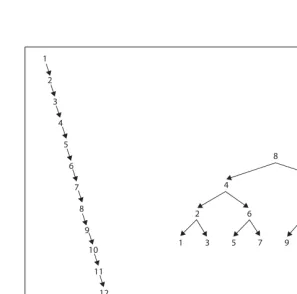
Knowing a bit about trees and how they behave, Gary asked Graham the $64,000 (it is logarithmic, after all) question: “Are you balancing the binary tree?” Graham’s response was surprising, since he was a very good software developer. “No, why should I do that? It makes the code a lot more complex.” But the fact that Graham wasn’t balancing the tree was exactly the problem causing the horrible performance of his code. Can you figure out why? Themalloc()routine in C allocates memory (from the heap) in order of increasing memory addresses. Not only are these addresses not evenly distributed, the order is exactly the one that leads to right-oriented trees, which behave more like linear lists than binary trees. To see why, consider the two binary trees in Figure 1-2. The (a) tree was created by inserting the numbers 1–15 in order. Its root node contains the value 1 and there is a path of 14 nodes to reach the node containing the value 15. The (b) tree was created by inserting these same numbers in the order <8, 4, 12, 2, 6, 10, 14, 1, 3, 5, 7, 9, 11, 13, 15>. In this case, the root node contains the value 8 but the paths to all other nodes in the tree are three nodes or less. As we will see in Chapter 5, the search time is directly affected by the length of the maximum path.

(18)

Algorithms to the Rescue

A balanced binary tree is a binary search tree for which the length of all paths from the root of the tree to any leaf node is as close to the same number as possible. Let’s definedepth(Li) to be the length of the path from the root of the

tree to a leaf nodeLi. In a perfectly balanced binary tree withnnodes, for any two

leaf nodes, L1 and L2, the absolute value of the difference, |depth(L2)–depth

(L1)|≤1; alsodepth(Li)≤log(n) for any leaf nodeLi.*Gary went to one of his

algo-rithms books and decided to modify Graham’s code so that the tree of allocation records would be balanced by making it a red-black binary tree. Red-black trees (Cormen et al., 2001) are an efficient implementation of a balanced binary tree in which given any two leaf nodes L1 and L2, depth(L2)/depth(L1)≤2; also

depth(Li)≤2*log2(n+1) for any leaf nodeLi. In other words, a red-black tree is roughly

balanced, to ensure that no path is more than twice as long as any other path.

[image:18.612.100.398.105.399.2]

The changes took a few hours to write and test. When he was done, Gary showed Graham the result. They ran each of the three programs shown previously.

(19)

Side Story | 9

Algorithms

Matter

ProgramA and ProgramC took just a few milliseconds longer than ProgramB. The performance improvement reflected approximately a 5,000-fold speedup. This is what might be expected when you consider that the average number of nodes to visit drops from 500,000 to 20. Actually, this is an order of magnitude off: you might expect a 25,000-fold speedup, but that is offset by the computation over-head of balancing the tree. Still, the results are dramatic, and Graham’s memory leak detector could be released (with Gary’s modifications) in the next version of the product.

Side Story

Given the efficiency of using red-black binary trees, is it possible that themalloc()

implementation itself is coded to use them? After all, the memory allocation func-tionality must somehow maintain the set of allocated regions so they can be safely deallocated. Also, note that each of the programs listed previously make alloca-tion requests for 32 bytes. Does the size of the request affect the performance of

malloc()andfree()requests? To investigate the behavior ofmalloc(), we ran a set of experiments. First, we timed how long it took to allocate 4,096 chunks ofn bytes, withnranging from 1 to 2,048. Then, we timed how long it took to deallo-cate the same memory using three strategies:

freeUp

In the order in which it was allocated; this is identical to ProgramC

freeDown

In the reverse order in which it was allocated

freeScattered

In a scattered order that ultimately frees all memory

For each value ofnwe ran the experiment 100 times and discarded the best and worst performing runs. Figure 1-3 contains the average results of the remaining 98 trials. As one might expect, the performance of the allocation follows a linear trend—as the size ofn increases, so does the performance, proportional ton. Surprisingly, the way in which the memory is deallocated changes the perfor-mance.freeUphas the best performance, for example, whilefreeDownexecutes about four times as slowly.

The empirical evidence does not answer whethermalloc()andfree()use binary trees (balanced or not!) to store information; without inspecting the source for

free(), there is no easy explanation for the different performance based upon the order in which the memory is deallocated.

(20)

The Moral of the Story

[image:20.612.102.397.117.518.2]

The previous story really happened. Algorithms do matter. You might ask whether the tree-balancing algorithm was the optimal solution for the problem. That’s a great question, and one that we’ll answer by asking another question: does it really matter? Finding the right algorithm is like finding the right solution

(21)

References | 11

Algorithms

Matter

work well enough. You must balance the cost of the solution against the value it adds. It’s quite possible that Gary’s implementation could be improved, either by optimizing his implementation or by using a different algorithm. However, the performance of the memory leak detection software was more than acceptable for the intended use, and any additional improvements would have been unproduc-tive overhead.

The ability to choose an acceptable algorithm for your needs is a critical skill that any good software developer should have. You don’t necessarily have to be able to perform detailed mathematical analysis on the algorithm, but you must be able to understand someone else’s analysis. You don’t have to invent new algorithms, but you do need to understand which algorithms fit the problem at hand. This book will help you develop these capabilities. When you have them, you’ve added another tool to your software development toolkit.

References

Cormen, Thomas H., Charles E. Leiserson, Ronald L. Rivest, and Clifford Stein,

(22)

Chapter 2 The Math of Algorithms

2 The Mathematics of

Algorithms

In choosing an algorithm to solve a problem, you are trying to predict which algo-rithm will be fastest for a particular data set on a particular platform (or family of platforms). Characterizing the expected computation time of an algorithm is inherently a mathematical process. In this chapter we present the mathematical tools behind this prediction of time. Readers will be able to understand the various mathematical terms throughout this book after reading this chapter. A common theme throughout this chapter (and indeed throughout the entire book) is that all assumptions and approximations may be off by a constant, and ultimately our abstraction will ignore these constants. For all algorithms covered in this book, the constants are small for virtually all platforms.

Size of a Problem Instance

An instance of a problem is a particular input data set to which a program is applied. In most problems, the execution time of a program increases with the size of the encoding of the instance being solved. At the same time, overly compact representations (possibly using compression techniques) may unneces-sarily slow down the execution of a program. It is surprisingly difficult to define the optimal way to encode an instance because problems occur in the real world and must be translated into an appropriate machine representation to be solved on a computer. Consider the two encodings shown in the upcoming sidebar, “Instances Are Encoded,” for a numberx.

(23)

Size of a Problem Instance | 13

The Math of

Algorithms

Selecting the representation of a problem instance depends on the type and variety of operations that need to be performed. Designing efficient algorithms often starts by selecting the proper data structures in which to represent the problem to be solved, as shown in Figure 2-1.

Instances Are Encoded

Suppose you are given a large numberxand want to compute the parity of the number of 1s in its binary representation (that is, whether there is an even or odd number of 1s). For example, ifx=15,137,300,128, its base 2 representation is:

x₂=1110000110010000001101111010100000

and its parity is even. We consider two possible encoding strategies: Encoding 1 ofx: 1110000110010000001101111010100000

Here, the 34-bit representation of x in base 2 is the representation of the problem and so the size of the input isn=34. Note thatlog2(x) is y≅33.82, so

this encoding is optimal. However, to compute the parity of the number of 1s, every bit must be probed. The optimal time to compute the parity grows linearly withn (logarithmically withx).

xcan also be encoded as ann-bit number plus an extra checksum bit that shows the parity of the number of 1s in the encoding ofx.

Encoding 2 ofx: 1110000110010000001101111010100000[0]

The last bit ofx in Encoding 2 is a 0 reflecting the fact thatxhas an even number of 1s (even parity=0). For this representation,n=35. In either case, the size of the encoded instance,n, grows logarithmically withx. However, the time for an optimal algorithm to compute the parity ofxwith Encoding 1 grows loga-rithmically with the size of the encoding ofx, and with Encoding 2 the time for an optimal algorithm is constant and doesn’t depend on the size of the encoding ofx.

Figure 2-1. More complex encodings of a problem instance

(24)

Because we cannot formally define the size of an instance, we assume that an instance is encoded in some generally accepted, concise manner. For example, when sortingn numbers, we adopt the general convention that each of the n numbers fits into a word in the platform, and the size of an instance to be sorted is

n. In case some of the numbers require more than one word—but only a constant, fixed number of words—our measure of the size of an instance is off by a constant. So an algorithm that performs a computation using integers stored in 64 bits may take twice as long as a similar algorithm coded using integers stored in 32 bits.

To store collections of information, most programming languages support arrays, contiguous regions of memory indexed by an integerito enable rapid access to theith_{element. An array is one-dimensional when each element fits into a word in} the platform (for example, an array of integers, Boolean values, or characters). Some arrays extend into multiple dimensions, enabling more interesting data representations, as shown in Figure 2-1. And, as shown in the upcoming sidebar, “The Effect of Encoding on Performance,” the encoding could affect an algo-rithm’s performance.

Because of the vast differences in programming languages and computer plat-forms on which programs execute, algorithmic researchers accept that they are unable to compute with pinpoint accuracy the costs involved in using a particular encoding in an implementation. Therefore, they assert that performance costs that differ by a multiplicative constant are asymptotically equivalent. Although such a definition would be impractical for real-world situations (who would be satisfied to learn they must pay a bill that is 1,000 times greater than expected?), it serves as the universal means by which algorithms are compared. When implementing an algorithm as production code, attention to the details reflected in the constants is clearly warranted.

Rate of Growth of Functions

The widely accepted method for describing the behavior of an algorithm is to represent the rate of growth of its execution time as a function of the size of the input problem instance. Characterizing an algorithm’s performance in this way is an abstraction that ignores details. To use this measure properly requires an awareness of the details hidden by the abstraction.

Every program is run on aplatform, which is a general term meant to encompass:

• The computer on which the program is run, its CPU, data cache, floating-point unit (FPU), and other on-chip features

• The programming language in which the program is written, along with the compiler/interpreter and optimization settings for generated code

• The operating system

• Other processes being run in the background

(25)

algo-Rate of Growth of Functions | 15

The Math of

Algorithms

distinct elements, one at a time, until a desired value, v, is found. For now, assume that:

• There aren distinct elements in the list • The element being sought,v, is in the list

• Each element in the list is equally likely to be the valuev

To understand the performance of SEQUENTIAL SEARCH, we must know how many elements it examines “on average.” Sincevis known to be in the list and each element is equally likely to bev, the average number of examined elements,

E(n), is the sum of the number of elements examined for each of thenvalues divided byn. Mathematically:

The Effect of Encoding on Performance

Assume a program stored information about the periodic table of elements. Three questions that frequently occur are a)“What is the atomic weight of element numberN?”, b)“What is the atomic number of the element namedX?”, and c)“What is the name of element numberN?”. One interesting challenge for this problem is that as of January 2008, element 117 had not yet been discov-ered, although element 118, Ununoctium, had been.

Encoding 1 of periodic table: store two arrays,elementName[], whoseithvalue stores the name of the element with atomic number i, and elementWeight[], whoseith value stores the weight of the element.

Encoding 2 of periodic table: store a string of 2,626 characters representing the entire table. The first 62 characters are:

1 H Hydrogen 1.00794 2 He Helium 4.002602 3 Li Lithium 6.941

The following table shows the results of 32 trials of 100,000 random query invoca-tions (including invalid ones). We discard the best and worst results, leaving 30 trials whose average execution time (and standard deviation) are shown in milliseconds:

Weight Number Name

Enc1 2.1±5.45 131.73±8.83 2.63±5.99 Enc2 635.07±41.19 1050.43±75.60 664.13±45.90

As expected, Encoding 2 offers worse performance because each query involves using string manipulaton operations. Encoding 1 can efficiently processweightand

name queries butnumber queries require an unordered search through the table. This example shows how different encodings result in vast differences in execu-tion times. It also shows that designers must choose the operaexecu-tions they would like to optimize.

E n( ) 1_n--- i

i=1

n

∑

n n( +1) 2n --- 1

2 ---n 1

2 ---+

(26)

Thus, SEQUENTIALSEARCHexamines about half of the elements in a list of n distinct elements subject to these assumptions. If the number of elements in the list doubles, then SEQUENTIAL SEARCHshould examine about twice as many elements; the expected number of probes is a linear function ofn. That is, the expected number of probes islinear or “about”c*nfor some constantc. Here,

c=1/2. A fundamental insight of performance analysis is that the constant c is unimportant in the long run, since the most important cost factor is the size of the problem instance,n. Asn gets larger and larger, the error in claiming that:

becomes less significant. In fact, the ratio between the two sides of this approxi-mation approaches 1. That is:

although the error in the estimation is significant for small values ofn. In this context we say that the rate of growth of the expected number of elements that SEQUENTIALSEARCHexamines is linear. That is, we ignore the constant multi-plier and are concerned only when the size of an instance is large.

When using the abstraction of the rate of growth to choose between algorithms, we must be aware of the following assumptions:

Constants matter

That’s why we use supercomputers and upgrade our computers on a regular basis.

The size of n is not always large

We will see in Chapter 4 that the rate of growth of the execution time of QUICKSORTis less than the rate of growth of the execution time of INSER-TIONSORT. Yet INSERTIONSORToutperforms QUICKSORTfor small arrays on the same platform.

An algorithm’s rate of growth determines how it will perform on increasingly larger problem instances. Let’s apply this underlying principle to a more complex example.

Consider evaluating four sorting algorithms for a specific sorting task. The following performance data was generated by sorting a block ofnrandom strings. For string blocks of sizen=1–512, 50 trials were run. The best and worst perfor-mances were discarded, and the chart in Figure 2-2 shows the average running time (in microseconds) of the remaining 48 results. The variance between the runs is surprising.

One way to interpret these results is to try to design a function that will predict the performance of each algorithm on a problem instance of size n. Since it is unlikely that we will be able to guess such a function, we use commercially

1 2 ---n 1

2 ---n 1

2 ---+ ≈ 1 2 ---n ⎝ ⎠ ⎛ ⎞ 1 2 ---n 1

2 ---+ ⎝ ⎠ ⎛ ⎞

(27)

Rate of Growth of Functions | 17

The Math of

Algorithms

regression analysis. The “fitness” of a trend line to the actual data is based on a value between 0 and 1, known as the R2_{value. Values near 1 indicate a high} fitness. For example, if R2_{= 0.9948, there is only a 0.52% chance that the fitness} of the trend line is due to random variations in the data.

SORT-4 is clearly the worst performing of these sort algorithms. Given the 512 data points as plotted in a spreadsheet, the trend line to which the data conforms is:

[image:27.612.97.442.94.488.2]

y = 0.0053*n2_–0.3601*_n_+39.212 R2_{= 0.9948}

(28)

Having an R2_{confidence value so close to 1 declares this is an accurate estimate.} SORT-2 offers the fastest implementation over the given range of points. Its behavior is characterized by the following trend line equation:

y = 0.05765*n*log(n)+7.9653

SORT-2 marginally outperforms SORT-3 initially, and its ultimate behavior is perhaps 10% faster than SORT-3. SORT-1 shows two distinct behavioral patterns. For blocks of 39 or fewer strings, the behavior is characterized by:

y = 0.0016*n2_+0.2939*_n_+3.1838

R2_{= 0.9761}

However, with 40 or more strings, the behavior is characterized by:

y = 0.0798*n*log(n)+142.7818

The numeric coefficients in these equations are entirely dependent upon the

plat-form on which these implementations execute. As described earlier, such incidental differences are not important. The long-term trend asnincreases domi-nates the computation of these behaviors. Indeed, Figure 2-2 graphs the behavior using two different ranges to show that the real behavior for an algorithm may not be apparent untiln gets large enough.

Algorithm designers seek to understand the behavioral differences that exist between algorithms. The source code for these algorithms is available from open source repositories, and it is instructive to see the impact of these designers’ choices on the overall execution. SORT-1 reflects the performance of qsorton Linux 2.6.9. When reviewing the source code (which can be found through any of the available Linux code repositories*_{), one discovers the following comment:} “Qsort routine from Bentley & McIlroy’s Engineering a Sort Function.” Bentley and McIlroy (1993) describe how to optimize QUICKSORTby varying the strategy for problem sizes less than 7, between 8 and 39, and for 40 and higher. It is satis-fying to see that the empirical results presented here confirm the underlying implementation.

Analysis in the Best, Average, and Worst Cases

One question to ask is whether the results of the previous section will be true for all input problem instances. Perhaps SORT-2 is only successful in sorting a small number of strings. There are many ways the input could change:

• There could be 1,000,000 strings. How does an algorithm scale to large input? • The data could be partially sorted, meaning that almost all elements are not

that far from where they should be in the final sorted list. • The input could contain duplicate values.

(29)

Analysis in the Best, Average, and Worst Cases | 19

The Math of

Algorithms

Although SORT-4 from Figure 2-2 was the slowest of the four algorithms for sortingnrandom strings, it turns out to be the fastest when the data is already sorted. This advantage rapidly fades away, however, with just 16 random items out of position, as shown in Figure 2-3.

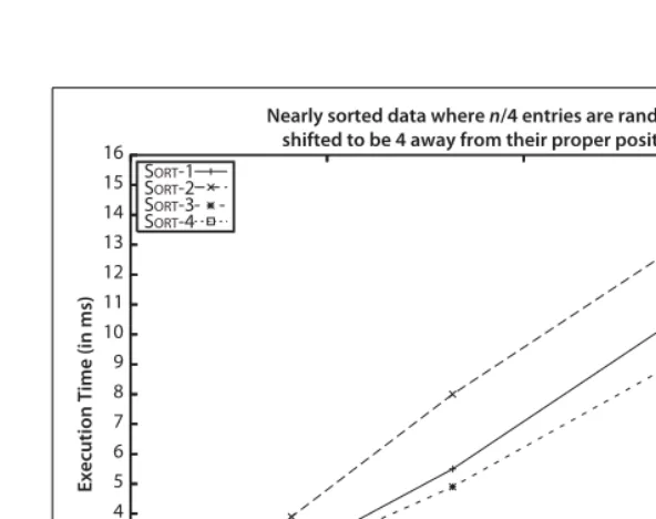
However, suppose an input array withnstrings is “nearly sorted”—that is,n/4 of the strings (25% of them) are swapped with another position just four locations away. It may come as a surprise to see in Figure 2-4 that SORT-4 outperforms the others.

[image:29.612.99.440.167.462.2]

The conclusion to draw is that for many problems, no single optimal algorithm exists. Choosing an algorithm depends on understanding the problem being solved and the underlying probability distribution of the instances likely to be treated, as well as the behavior of the algorithms being considered.

(30)

To provide some guidance, algorithms are typically presented with three common cases in mind:

Worst-case

Defines a class of input instances for which an algorithm exhibits its worst runtime behavior. Instead of trying to identify the specific input, algorithm designers typically describepropertiesof the input that prevent an algorithm from running efficiently.

Average-case

Defines the expected behavior when executing the algorithm on random input instances. Informally, while some input problems will require greater time to complete because of some special cases, the vast majority of input problems will not. This measure describes the expectation an average user of the algorithm should have.

Best-case

Defines a class of input instances for which an algorithm exhibits its best runtime behavior. For these input instances, the algorithm does the least work. In reality, the best case rarely occurs.

[image:30.612.101.397.112.346.2]

By knowing the performance of an algorithm under each of these cases, you can judge whether an algorithm is appropriate for use in your specific situation.

(31)

Analysis in the Best, Average, and Worst Cases | 21

The Math of

Algorithms

Worst-Case

Asngrows, most problems have a greater number of potential instances of sizen. For any particular value ofn, the work done by an algorithm or program may vary dramatically over all the instances of sizen. For a given program and a given value

n, the worst-case execution time is the maximum execution time, where the maximum is taken over all instances of sizen.

Paying attention to the worst case is a pessimistic view of the world. We are inter-ested in the worst-case behavior of an algorithm because of:

The desire for an answer

This often is the easiest analysis of the complexity of an algorithm.

Real-time constraints

If you are designing a system to aid a surgeon performing open-heart surgery, it is unacceptable for the program to execute for an unusually long time (even if such slow behavior doesn’t happen “often”).

More formally, ifSnis the set of instancessiof sizen, andtmeasures the work

done by an algorithm on each instance, then work done by an algorithm onSnin

the worst case is the maximum oft(si) over allsi∈Sn. Denoting this worst-case

work on Sn by Twc(n), the rate of growth of Twc(n) defines the worst-case

complexity of the algorithm.

In general, there are not enough resources to compute each individual instancesi

on which to run the algorithm to determine empirically the input problem that leads to worst-case performance. Instead, an adversary tries to craft a worst-case input problem given the description of an algorithm.

Average-Case

A telephone system designed to support a large numbernof telephones must, in the worst case, be able to complete all calls wheren/2 people pick up their phones and call the othern/2 people. Although this system will never crash because of overload, it will be prohibitively expensive to construct. Besides, the probability that each ofn/2 people calls a unique member of the othern/2 people is exceed-ingly small. One could design a system that is cheaper and will very rarely (possibly never) crash due to overload. But we must resort to mathematical tools to consider probabilities.

For the set of instances of sizen, we associate a probability distribution Pr, which assigns a probability between 0 and 1 to each instance such that the sum, over all instances of sizen, of the probability of that instance is 1. More formally, ifSnis

the set of instances of sizen, then:

Pr{ }si si

∑

∈Sn

(32)

Iftmeasures the work done by an algorithm on each instance, then the average-case work done by an algorithm onSn is:

That is, the actual work done on instancesi,t(si), is weighted with the probability

thatsiwill actually be presented as input. If Pr{si}=0, then the actual value oft(si)

does not impact the expected work done by the program. Denoting this average-case work onSnbyTac(n), then the rate of growth ofTac(n) defines the

average-case complexity of the algorithm.

Recall that when describing the rate of growth of work or time, we consistently ignore constants. So when we say that SEQUENTIALSEARCHofnelements takes, on average:

probes (subject to our earlier assumptions), then by convention we simply say that subject to these assumptions, we expect SEQUENTIALSEARCHwill examine a

linear number of elements, ororder n.

Best-Case

Knowing the best case for an algorithm is useful even though the situation rarely occurs in practice. In many cases, it provides insight into the optimal circum-stance for an algorithm. For example, the best case for SEQUENTIALSEARCHis when it searches for a desired value,v, which ends up being the first element in the list. A slightly different approach, which we’ll call COUNTING SEARCH, searches for a desired value,v, and counts the number of times thatvappears in the list. If the computed count is zero, then the item was not found, so it returns

false; otherwise, it returnstrue. Note that COUNTINGSEARCHalways searches through the entire list; therefore, even though its worst-case behavior is O(n)—the same as SEQUENTIAL SEARCH—its best-case behavior remains O(n), so it is unable to take advantage of either the best-case or average-case situations in which it could have performed better.

Performance Families

We compare algorithms by evaluating their performance on input data of sizen. This methodology is the standard means developed over the past half-century for comparing algorithms. By doing so, we can determine which algorithms scale to solve problems of a nontrivial size by evaluating the running time needed by the algorithm in relation to the size of the provided input. A secondary form of perfor-mance evaluation is to consider how much memory or storage an algorithm needs; we address these concerns within the individual algorithm chapters, as appropriate.

Tac( )n

1

Sn

--- t s( )_i Pr{ }si si

∑

∈Sn

=

1 2 ---n 1

(33)

Performance Families | 23

The Math of

Algorithms

We use the following classifications exclusively in this book, and they are ordered by decreasing efficiency:

• Constant • Logarithmic • Sublinear • Linear • n log (n) • Quadratic • Exponential

We’ll now present several discussions to illustrate some of these performance identifications.

Discussion 0: Constant Behavior

When analyzing the performance of the algorithms in this book, we frequently claim that some primitive operations provide constant performance. Clearly this claim is not an absolute determinant for the actual performance of the operation since we do not refer to specific hardware. For example, comparing whether two 32-bit numbersxand yare the same value should have the same performance regardless of the actual values ofxandy. A constant operation is defined to have O(1) performance.

What about the performance of comparing two 256-bit numbers? Or two 1,024-bit numbers? It turns out that for a predetermined fixed sizek, you can compare twok-bit numbers in constant time. The key is that the problem size (i.e., the values of the numbersxandythat are being compared) cannot grow beyond the fixed sizek. We abstract the extra effort, which is multiplicative in terms ofk, with the notation O(1).

Discussion 1: Log n Behavior

A bartender offers the following $10,000 bet to any patron. “I will choose a number from 1 to 1,000,000 and you can guess 20 numbers, one at a time; after each guess, I will either tell you TOO LOW, TOO HIGH, or YOU WIN. If you win in 20 questions, I give you $10,000; otherwise, you give me $10,000.” Would you take this bet? You should because you can always win. Table 2-1 shows a sample scenario for the range 1–10 that asks a series of questions, reducing the problem size by about half each time.

Table 2-1. Sample behavior for guessing number from 1–10

Number First guess Second guess Third guess

1 Is it 5?

TOO HIGH Is it 2?TOO HIGH Is it 1?YOU WIN

2 Is it 5?

TOO HIGH Is it 2?YOU WIN

(34)

In each turn, depending upon the specific answers from the bartender, the size of the potential range containing the hidden number is cut in about half each time. Eventually, the range of the hidden number will be limited to just one possible number; this happens after⎡log (n)⎤turns. The ceiling function ⎡x⎤rounds the numberxup to the smallest integer greater than or equal tox. For example, if the bartender chooses a number between 1 and 10, you could guess it in⎡log (10)⎤= ⎡3.32⎤, or four guesses, as shown in the table.

This same approach works equally well for 1,000,000 numbers. In fact, the GUESSINGalgorithm shown in Example 2-1 works for any range [low,high] and determines the value of nin⎡log (high–low+1)⎤ turns. If there are 1,000,000 numbers, this algorithm will locate the number in at most⎡log (1,000,000)⎤= ⎡19.93⎤, or 20 guesses (the worst case).

3 Is it 5?

TOO HIGH Is it 2?TOO LOW Is it 3?YOU WIN

4 Is it 5?

TOO HIGH Is it 2?TOO LOW Is it 3?TOO LOW, so it must be 4

5 Is it 5?

YOU WIN

6 Is it 5?

TOO LOW Is it 8?TOO HIGH Is it 6?YOU WIN

7 Is it 5?

TOO LOW Is it 8?TOO HIGH Is it 6?TOO LOW, so it must be 7

8 Is it 5?

TOO LOW Is it 8?YOU WIN

9 Is it 5?

TOO LOW Is it 8?TOO LOW Is it 9?YOU WIN

10 Is it 5?

TOO LOW Is it 8?TOO LOW Is it 9?TOO LOW, so it must be 10

Example 2-1. Java code to guess number in range [low,high]

// Compute number of turns when n is guaranteed to be in range [low,high]. public static int turns(int n, int low, int high) {

int turns = 0;

// While more than two potential numbers remain to be checked, continue. while (high – low≤2) {

// Prepare midpoint of [low,high] as the guess. turns++;

int mid = (low + high)/2; if (mid == n) {

return turns; } else if (mid < n) { low = mid + 1;

Table 2-1. Sample behavior for guessing number from 1–10 (continued)

(35)

Performance Families | 25

The Math of

Algorithms

Logarithmicalgorithms are extremely efficient because they rapidly converge on a solution. In general, these algorithms succeed because they reduce the size of the problem by about half each time. The GUESSING algorithm reaches a solution after at mostk=⎡log (n)⎤ iterations, and at theith_{iteration (}_i_{>0), the algorithm} computes a guess that is known to be within ±ε=2k–i _{from the actual hidden} number. The quantityεis considered the error, or uncertainty. After each itera-tion of the loop,ε is cut in half.

Another example showing efficient behavior is Newton’s method for computing the roots of equations in one variable (in other words, for what values ofxdoes

f(x) = 0?). To find whenx*sin(x)–5*x=cos(x), setf(x)=x*sin(x)–5*x–cos(x) and its derivative f’(x)=x*cos(x)+sin(x)–5–sin(x)=x*cos(x)–5. The Newton iteration computes xn+1=xn–f(xn)/f’(xn). Starting with a “guess” that xis zero, this

algo-rithm quickly determines an appropriate solution ofx=–0.189302759, as shown in Table 2-2. The binary and decimal digits enclosed in brackets, [], are the accu-rate digits.

Discussion 2: Sublinear O(n

d

_{) Behavior for d<1}

In some cases, the behavior of an algorithm is better thanlinear, yet not as effi-cient aslogarithmic. As discussed in Chapter 9, the kd-tree in multiple dimensions can partition a set ofnd-dimensional points efficiently. If the tree is balanced, the search time for range queries that conform to the axes of the points is O(n1–1/d_).

Discussion 3: Linear Performance

Some problems clearly seem to require more effort to solve than others. Any eight-year-old can evaluate 7+5 to get 12. How much harder is the problem 37+45? }

}

// At this point, only two numbers remain. We guess one, and if it is // wrong then the other one is the target. Thus only one more turn remains. return 1 + turns;

}

Table 2-2. Newton’s method

n x_n in decimal x_n in bits (binary digits)

0 0.0

1 –0.2 [1011111111001]0011001100110011001100110…

2 –[0.18]8516717588… [1011111111001000001]0000101010000110110…

3 –[0.1893]59749489… [101111111100100000111]10011110000101101…

4 –[0.189]298621848… [10111111110010000011101]011101111111011…

5 –[0.18930]3058226… [1011111111001000001110110001]0101001001…

6 –[0.1893027]36274… [1011111111001000001110110001001]0011100…

7 –[0.189302759]639… [101111111100100000111011000100101]01001…

(36)

In general, how hard is it to add twon-digit numbersan…a1+bn…b1to result in

acn+1…c1digit value? The primitive operations used in this ADDITIONalgorithm

are as follows:

A sample Java implementation of ADDITIONis shown in Example 2-2, where an

n-digit number is represented as an array ofintvalues; for the examples in this section, it is assumed that each of these values is a decimal digit d such that 0≤d≤9.

As long as the input problem can be stored in memory,addcomputes the addi-tion of the two numbers as represented by the input integer arraysn1andn2. Would this implementation be as efficient as the followinglastalternative, listed in Example 2-3?

Example 2-2. Java implementation of add

public static void add (int[] n1, int[] n2, int[] sum) { int position = n1.length-1;

int carry = 0; while (position >= 0) {

int total = n1[position] + n2[position] + carry; sum[position+1] = total % 10;

if (total > 9) { carry = 1; } else { carry = 0; } position--;

}

sum[0] = carry; }

Example 2-3. Java implementation of last

public static void last(int[] n1, int[] n2, int[] sum) { int position = n1.length;

int carry = 0;

while (--position >= 0) {

int total = n1[position] + n2[position] + carry; if (total > 9) {