Flow control on helicopter rotors using active gurney flaps

(1)

Flow Control on Helicopter Rotors Using Active

Gurney Flaps

Thesis submitted in accordance with the requirements of the University of Liverpool for the degree of Doctor of Philosophy

by

Vasileios Pastrikakis

(2)

(3)

Declaration

I hereby declare that this dissertation is a record of work carried out in the School of Engineering at the University of Liverpool during the period from January 2012 to January 2015. The dissertation is original in content except where otherwise indicated.

February 2015

...

(4)

Abstract

This thesis presents closed loop control of active Gurney flaps on rotors. Firstly, it builds on the Helicopter Multi-Block 2 CFD solver of the University of Liverpool and demonstrates the imple-mentation and use of Gurney flaps on wings, and rotors. The idea is to flag any cell face within the computational mesh with a solid, no slip boundary condition. Hence the infinitely thin Gurney can be approximated by “blocking cells” in the mesh. Comparison between thick Gurney flaps and infinitely thin Gurneys showed no difference on the integrated loads, the same flow structure was captured and the same vortices were identified ahead and behind the Gurney. The results presented for various test cases suggest that the method is simple and efficient and it can therefore be used for routine analysis of rotors with Gurney flaps.

The potential effect of a Gurney flap all over the performance of the W3-Sokol rotor blade in hover was studied next. A rigid blade was first considered and the calculations were conducted at several thrust settings. The Gurney flap was extended from 46%R to 66%R and it was located at the trailing edge of the main rotor blade. Four different sizes of Gurney flaps were studied, 2%, 1%, 0.5% and 0.3% of the chord, and the biggest flap proved to be the most effective. A second study considered elastic blades with and without the Gurney flap. The results were trimmed at the same thrust values as the rigid blade and indicate an increase of aerodynamic performance when the Gurney flap is used, especially for high thrust cases.

Moreover, the performance of the W3-Sokol rotor in forward flight with and without Gurney flap was tested. Rigid and elastic blade models were considered and calculations were guided using flight test data. The Gurney flap was extended from 40%R to 65%R, while the size of the Gurney was selected to be 2% of the chord based on the hover study. All results were trimmed to the same thrust as flight tests. The harmonic analysis of the flight test data proved to be a useful tool for identifying vibrations on the rotor caused by stall at the retreating side, and a carefully designed Gurney flap and actuation schedule were essential to alleviate the effects of flow separation.

The last part of the thesis is dedicated to a closed loop actuation of the Gurney flap based on the leading edge pressure divergence criterion. The effect of the Gurney flap on the trimming of a full helicopter model, as well as the handling qualities of the rotorcraft were investigated.

(5)

Publications

Book Chapter

V. Pastrikakis, R. Steijl and G. Barakos, Computational Aeroelastic Analysis of a

Hovering W3 Sokol Blade with Gurney Flap,

Springer Book “Advances in

Fluid-Structure Interaction", considered for publication.

Journal Papers

V. Pastrikakis, R. Steijl and G. Barakos, Alleviation of retreating side stall using

active Gurney flaps on rotors,

Accepted in AIAA Journal of Aircraft

, February 2015.

M. Woodgate, V. Pastrikakis and G. Barakos, A Method for Calculating Rotors with

Active Gurney Flaps,

Accepted in AIAA Journal of Aircraft

, January 2015.

V. Pastrikakis, R. Steijl, G. Barakos, and J. Malecki, Computational Aeroelastic

Analysis of a Hovering W3 Sokol Blade with Gurney Flap,

Journal of Fluids and

Structures

, Number:1763, July 2014.

Papers in Conference Proceedings

V. Pastrikakis, R. Steijl and G. Barakos, Effect of Active Gurney Flaps on the Overall

Helicopter Flight Envelope,

Submitted to 41st European Rotorcraft Forum, Munich,

Germany, 1–4 September

, 2015.

V. Pastrikakis, R. Steijl and G. Barakos, Alleviation of retreating side stall using

active elements for helicopter rotors,

40th European Rotorcraft Forum, Southampton,

United Kingdom, 2–5 September

, 2014.

V. Pastrikakis, R. Steijl and G. Barakos, Computational Analysis of the W3 Sokol

Rotor with Gurney Flaps,

39th European Rotorcraft Forum, Moscow, Russian

Federation, 3–6 September

, 2013.

M. Woodgate, V. Pastrikakis and G. Barakos, Rotor Computations with Active

Gurney Flaps,

ERCOFTAC international symposium "Unsteady separation in

fluid-structure interaction", Mykonos, Greece, June

, 2013.

Technical Reports

V. Pastrikakis, Post-Processing Forward Flying Rotors, Technical Note TN13-007,

2013.

V. Pastrikakis, Computations using virtual Gurney flaps, Technical Note TN14-002,

2014.

(6)

Reports under the IMESCON

“W3-Sokol flight test data processing", November 2012

“Mid-Term Report - University of Liverpool Contribution to IMESCON", May 2013

“Optimal Gurney flap for W3-Sokol in hover", September 2013

“Optimal Gurney flap for W3-Sokol in forward flight", February 2015

“Final Report - University of Liverpool Contribution to IMESCON", February 2015

Training under the IMESCON

Workshop “Principles on helicopter Engineering"Gdansk - Lublin, Poland, April

2012.

Summer School in “Computational Fluid Dynamics",Gdansk, Poland, July 2012.

Workshop “LMS Ground Vibration Testing (GVT) Master Class", Leuven, Belgium,

September 2012.

Short course in Parallel Computing with MPI by NAG, Liverpool, UK, October 2012.

Workshop “Multiple physics simulation codes coupling for FSI", Liverpool, UK,

October 2013.

Workshop “Finite Element Method", Gdansk, Poland, June 2014.

Summer School “Multi-physics Simulation", Liverpool, UK, July 2014.

Advanced Training on FLIGHTLAB by Advanced Rotorcraft Technologies,

Liverpool, UK, February 2015.

Placements

(7)

Acknowledgements

My deepest gratitude should be devoted to my first supervisor Prof. George Barakos. His tech-nical knowledge, encouragement and support kept me motivated and made this thesis a reality. I would also like to thank my second supervisor Dr. René Steijl for being a great mentor and sharing his knowl-edge constantly. Special thanks for Dr. Mark Woodgate for the numerous discussions we had, and for all those times that he helped me solve my computational problems. The CFD lab felt like second home all these years and the time spent with other members of this lab and others (Nick Tantaroudas, Dr. George Zografakis, Dr. Evangelos Papatheou, George Hoholis, Vladimir Leble, Antonio Jimenez Garcia) is of great value.

The financial support via the IMESCON project, the release of data crucial for this study by the leading specialist for aeromechanics and dynamics of PZL Swidnik, Jacek Malecki, the use of the computing centre TASK (Gdansk, Poland) and Chadwick (University of Liverpool, UK) are gratefully acknowledged.

Moreover, I would like to highlight the significance of European Initial Training Networks, and thank all the fellows who worked with me and exchanged a lot of ideas to complete IMESCON project successfully.

Many thanks should go to Dr. William Maybury from Axsym-engineering, and Karl Baverstock from AgustaWestland for introducing me to the exciting rotorcraft industry. Our discussions gave me additional motivation for success.

(8)

(9)

List of Figures

1.1 Rotor disk showing velocities in forward flight. View from top. . . 2

1.2 Classification of flow control strategies. . . 5

1.3 Interrelation between flow control goals. . . 7

1.4 Optimising for dynamic stall control - Bousman’s dynamic stall function. . . 8

1.5 Array of counter rotating triangular vortex generators. . . 10

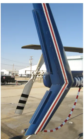
1.6 Double Gurney flaps on a Bell 222U helicopter vertical stabiliser (wikipedia). . . 18

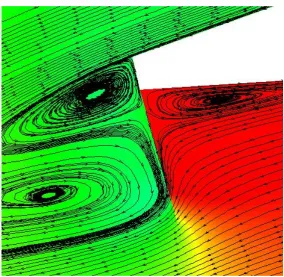
1.7 CFD visualisation of the flow pattern at the trailing edge with a Gurney flap. . . 19

1.8 Applying a voltage to a piezoceramic wafer. . . 22

1.9 Gurney flap actuation mechanism mounted inside the W3-Sokom main rotor blade. . . 22

2.1 Proposed Gurney flap configurations. . . 37

2.2 The 3 possible methods for the solution of the active Gurney flap shown for configura-tion (b) of Figure 2.1. . . 38

2.3 Example of a possible blocking for a Gurney at 95% of the chord. (b) shows a closeup of the Gurney flap. NACA0012 aerofoil, Gurney size = 2% chord, Gurney thickness = 0.25% chord . . . 39

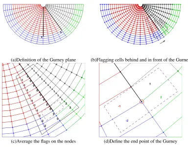
2.4 Method for flagging a Gurney flap. (I) Gurney plane definition, and (II) elimination of block boundaries 3 and 4 for not meeting the distance requirements, and part of boundaries 1 and 2 for not meeting the angle requirements. Only the cell faces of the accepted block boundaries which are inside the Gurney plane will be flagged as solid (Gurney flap). . . 40

2.5 Flagging of the cells - shaded - that require a wall boundary condition applied to their face in order to model the Gurney flap (shown in solid black line). The Gurney flap can change in length without a change in the cells flagged as blocked. Minimal changes are needed in the CFD mesh (g), (h), and the Gurney flap can be seen in (i). . . 41

2.6 Part-flux method description. (a) a schematic of a Gurney flap covered part of the face between two cells, and (b) calculation of the fluxes twice before weighting them. . . . 44

2.7 Lift coefficient comparison between the part-flux (method 1) and the full-flux (method 0) methods for a NACA 0012 aerofoil with an actuated 2% chord Gurney flap.M=0.2, Re=2.1x106_,_α₌₀o_{, k-}_ω_{SST. . . .} ₄₅

2.8 Viscous flow around a NACA 0012 aerofoil with an actuated 2% chord Gurney flap. The colour contours represent the solution with the full flux method and the white contours represent the solution with part-fluxes.M=0.2,Re=2.1x106,α=0o, k-ω SST. . . . 45

2.9 Example of a possible blocking for a Swinging Gurney at 95% of the chord, and a near view of the topology. . . 46

2.10 Description of method for flagging wall faces for a swinging Gurney case with HMB2. 47 2.11 Two overset grids covering the domain around an aerofoil. . . 54

2.12 Localisation pre-processing. . . 55

(14)

2.14 Range tree localisation schematic. For each cell of a chimera block, an AABB is created. It needs an input (inquiry) for the tree, which returns all the points located inside the box. This step is followed by an exactin-cellcheck for all the point returned by the tree, which are not flagged asnode-in-cell. . . 57 2.15 Flux calculation stencil. Each fringe needs two neighbours in each direction and all

edge neighbours for consistent flux calculation. . . 57

3.1 Blocking and mesh spacings for a Gurney at the trailing edge. . . 64 3.2 The pressure contours and streamlines for four different heights of Gurneys. NACA0012,

M=0.2,α=0o,Re=2.1x106, k-ωSST. . . 65 3.3 Successive views of the flow near the aerofoil Gurney junction. Streamlines and

con-tours of Pressure coefficient are shown. . . 66 3.4 Flow visualisation behind an aerofoil, computed unsteady with a fixed, resolved Gurney

and wake.M=0.2,Re=2.1x106,α=0o, k-ωSST. . . 66 3.5 Comparison between thick and thin Gurneys for a NACA0012 aerofoil with a Gurney

of 2%c length computed at Mach number of 0.2 and zero incidence angle. Viscous computations were necessary for this case. Dotted line represents the case with the infinitely thin Gurney flap. . . 67 3.6 Comparison of loads for different Gurney heights at the trailing edge against

experimen-tal data. . . 67 3.7 Comparison of pressure distribution of a 2% Gurney at the trailing edge for different

angles of attack. . . 68 3.8 Definition of the actuation of the virtual Gurney used for NACA23012M aerofoil with

cavity. . . 68 3.9 (a) Lift, (b) drag, and (c) moment coefficients comparison on NACA23012M aerofoil

with cavity and a linearly actuated virtual and thick Gurney flap of 1.5%c at 93.5%c, M=0.2,Re=0.5·106_. _{. . . .} ₆₉

3.10 Vorticity magnitude visualisation for a NACA23012M aerofoil with cavity and a linearly actuated virtual (a) and thick (b) Gurney flap of 1.5%c at 93.5%c, M=0.2,Re=0.5·106_.

The Gurney flap is fully retracted. . . 69 3.11 Vorticity magnitude visualisation for a NACA23012M aerofoil with cavity and a linearly

actuated virtual (a) and thick (b) Gurney flap of 1.5%c at 93.5%c, M=0.2,Re=0.5·106_.

The Gurney flap is half actuated. . . 69 3.12 Vorticity magnitude visualisation for a NACA23012M aerofoil with cavity and a linearly

actuated virtual (a) and thick (b) Gurney flap of 1.5%c at 93.5%c, M=0.2,Re=0.5·106_.

The Gurney flap is fully actuated. . . 70 3.13 Part-span Gurney flap on a wing. (a) overview and (b) close view of the Gurney flap and

the surface mesh. . . 70 3.14 Pressure coefficient behind a fixed (a) and an active (b) Gurney flap, and lift and drag

coefficients of the 3D wing computed unsteady with the fixed (c, e) and the active (d, f) part-span Gurney flap. . . 71 3.15 Pressure coefficient behind a swinging Gurney at 45 degrees (a) and at 135 degrees of

actuation (b), and Lift and Drag coefficients of the 3D wing computed unsteady with the swinging Gurney (c, d). . . 72 3.16 (a) NACA23012M wing with 20 pairs of counter rotating vortex generators, (b)

specifi-cation of vortex generator vane. . . 74 3.17 Overview of sliding planes used for grid refinement. . . 75 3.18 Overview of the mesh (a) near the vortex generators, and (b) near the trailing edge. . . 75 3.19 (a) NACA23012M wing with fixed Gurney flap at the trailing edge, and (b) a close view

of the flap and surface mesh near the trailing edge. . . 76 3.20 (a) Lift, and (b) drag, coefficients comparison between Gurney flap and vortex

genera-tors for a wing NACA23012M,M=0.2843,Re=1.72×106. . . 77 3.21 (a) Moment coefficient, and (b) lift over drag ratio comparison between Gurney flaps

(15)

3.22 Lift over drag ratio versus lift coefficient comparison between Gurney flaps and vortex generators for a wing NACA23012M,M=0.2843,Re=1.72×106. . . 79 3.23 Description of pitching translation wing simulating the forward flight effect of a rotor

section. . . 80 3.24 (a) Pitching, (b) translational motion, and (c) variation of the local velocity of the

NACA23012M wing. dMdt case is presented in Table 3.1. . . 81 3.25 (a)M2CL, (b) M2CD, (c) M2CM, and (d)L/Dcomparison for clean wing (black solid

line), wing with active Gurney flap (blue dashed line), and wing with vortex generators (green dashed-dotted line). dMdt case is presented in Table 3.1. . . 84 3.26 Visualisation of the streamlines along the span of the clean wing. The red line indicates

the onset of the separation. dMdt case is presented in Table 3.1. . . 85 3.27 Visualisation of the streamlines along the span of the wing with active Gurney flap. The

red and blue line indicates the onset of the separation on the clean wing and the wing with active Gurney respectively. dMdt case is presented in Table 3.1. . . 85 3.28 Visualisation of the streamlines along the span of the wing with vortex generators. The

dashed green line indicates the onset of the separation on the wing with the vortex gen-erators. dMdt case is presented in Table 3.1. . . 86

4.1 Visualisation of the inboard and outboard Gurneys on the UH60A rotor. . . 89

4.2 Surface pressure distribution on the UH60A hovering rotor with and without Gurney flaps.Mtip=0.63,Re=7.83x106. . . 90 4.3 Visualisation of the Gurney effect on the UH60A hovering rotor with contours of

pres-sure coefficient based on the tip speed and iso-lines of vorticity magnitude.Mtip=0.63,

Re=7.83x106_{. . . .} ₉₁

4.4 (I) Geometry of W3-Sokol MRB, (II) close view at the trim tab and the trailing edge tab, (III) close view at the tip. . . 93 4.5 CFD mesh and boundary conditions on W3 Sokol rotor in hover. . . 94 4.6 Figure of merit versus thrust coefficient for the W3 Sokol MRB in hover (Mtip=0.618,Retip=

3.74·106,σ=0.0714). . . 95 4.7 Torque versus thrust coefficient for the W3 Sokol MRB in hover (Mtip=0.618,Retip=

3.74·106,σ=0.0714). . . 96 4.8 Estimated benefit in hover flight when a Gurney flap is deployed (Mtip=0.618,Retip=

3.74·106,σ=0.0714). . . 96 4.9 (a) Pressure coefficient along the W3 MRB and (b) pressure coefficient at different

sec-tions of the blade normalised using the local dynamic head, θ=10o, β =5o,CT=

0.0132, FM=0.7432,CQ=0.001. . . 98

4.10 Wake visualisation on W3 MRB (a) with out and (b) with Gurney flap in hover by using the isosurface of vorticity magnitude equal to 0.1s−1_,_θ₌₁₀o_,_β₌₅o_,_C

T=0.0132,

FM=0.7432,CQ=0.001. . . 99

4.11 Pressure distribution on upper and lower surface of W3 MRB without Gurney. θ = 11.5o_,_β ₌₆o_,_C

T/σ=0.216, FM=0.6934,CQ=0.00138. . . 100

4.12 Pressure distribution on upper and lower surface of W3 MRB with Gurney.θ=10.46o_,

β=5.21o_,_C

T/σ=0.216, FM=0.7374,CQ=0.00129. . . 101

4.13 Pressure coefficient atr/R=0.56 - Comparison between clean blade and blade with Gurney flap. . . 102 4.14 Structural model of the W3 Sokol blade used in NASTRAN. . . 103 4.15 Structural properties of the W3 Sokol blade used in NASTRAN. . . 103 4.16 Convergence history for thrust coefficient, collective and coning angle during aeroelastic

(16)

4.18 (a) Sectional thrust coefficient, (b) pitching moment coefficient, and (c) torque coeffi-cient of the W3 MRB with (dashed line) and without Gurney flap (solid line). Clean blade: θ=11.5o,β =6o,CT/σ =0.216,FM=0.6934,CQ=0.00138. Blade with Gurney flap: θ =10.46o, β =5.21o,CT/σ =0.216, FM=0.7374,CQ=0.00129.

Gurney size = 2%c. . . 107

4.19 (a) Sectional thrust coefficient (b) pitching moment coefficient, and (c) torque coefficient of the W3 MRB with (dashed line) and without Gurney flap (solid line). Clean blade: θ=10.0o_,_β₌₅o_,_C T/σ=0.1853, FM=0.7432,CQ=0.001. Blade with Gurney flap: θ=9.15o_,_β ₌_4.16o_,_C T/σ=0.1853, FM=0.7429,CQ=0.001. Gurney size = 2%c. 108 4.20 (a) Sectional thrust coefficient, (b) pitching moment coefficient, and (c) torque coeffi-cient of the W3 MRB with (dashed line) and without Gurney flap (solid line). Clean blade:θ=14o_,_β₌_6.2o_,_C T/σ =0.264, FM=0.622,CQ=0.0021. Blade with Gur-ney flap: θ =12.92o_,_β ₌_7.36o_,_C T/σ=0.264, FM=0.656,CQ=0.0017. Gurney size = 2%c. . . 109

4.21 Change of twist distribution for W3 MRB with and without Gurney flap in hover. Gur-ney size = 2%c. . . 110

4.22 (a) Collective and (b) coning angle after trimming versusCT/σ for different Gurney sizes on the W3 MRB in hover. . . 110

4.23 Different tip shapes of S-76 blade. . . 113

4.24 Structural model of S-76 blade. . . 114

4.25 Mass distribution of different blades used for static computations. . . 114

4.26 Flapwise moment area of inertia of different blades used for static computations. . . . 115

4.27 Chordwise moment area of inertia of different blades used for static computations. . . 115

4.28 Torsional constant of different blades used for static computations. . . 116

4.29 Spoke diagram for S-76 blade, comparison between rectangular and tapered-swept tip design. . . 116

4.30 Spoke diagram for S-76 blade, comparison between rectangular and tapered tip design. 117 4.31 Spoke diagram for S-76 blade, comparison between rectangular and swept tip design. . 117

4.32 Vortex generated at the blade tip of W3 Sokol in hover. . . 118

4.33 Spoke diagram for W3-Sokol blade. Circles are used for blade with Gurney flap. . . . 119

4.34 W3 Sokol blade in hover using Chimera technique. . . 120

4.35 W3 Sokol blade mesh and Background mesh. . . 121

4.36 Overview of background mesh at the left, and close view of the two background meshes at the right. . . 121

4.37 Visualisation of vorticity isosurface with W-velocity contour and W3 Sokol blade with pressure distribution contour for the blade with fixed Gurney flap in hover,CT =0.012. 122 5.1 Schedule of pitching, flapping motion, and Gurney flap deployment around azimuth for UH60A in forward flight. 100% deployment represents Gurney size of 2.22% of the chord. . . 127

5.2 Comparison of loads between CFD and Experimental data for UH60-A in forward flight at r/R=0.675 and r/R=0.865. . . 128

5.3 Surface pressure coefficient on the UH60A rotor without and with Gurney flap based on theMtipof the blade atΨ=0o.M∞=0.2363,Re∞=5x106,µ=0.368. . . 129

5.6 Normal force coefficient for the UH60A elastic rotor in forward flight with and without active Gurney flap, Coarse mesh. . . 132

5.7 Moment coefficient for the UH60A elastic rotor in forward flight with and without active Gurney flap, Coarse mesh. . . 133

(17)

5.9 Integrated loads for the UH60A elastic rotor in forward flight with active Gurney flap

deployed in opposite direction (towards suction side) - coarse mesh. . . 135

5.10 Time domain flight parameters for forward flight with helicopter weight equals to 6400 kg. . . 136

5.11 Peak to peak values of torsional and flapping bending moment atr/R=0.23, helicopter weight equals to 6400 Kg. . . 137

5.12 Harmonic analysis of (a) torsional, (b) flapping, and (c) lagging moment of the first MR blade atr/R=0.23, helicopter weight equals to 6400 Kg. . . 138

5.13 Schedule for the feathering and flapping angle for the W3 Sokol MR blade in forward flight. Case conditions are presented in Table 5.3. . . 139

5.14 Pressure distribution and vorticity magnitude visualisation at r/R=0.45 of the W3 Sokol blade in forward flight at (a)Ψ=210o, (b)Ψ=250o, (c)Ψ=270o, and (d) Ψ=310o_{. Case conditions are presented in Table 5.3. . . .} ₁₄₀

5.15 (a) Stall map of W3 Sokol blade in forward flight, and (b) actuation schedule of gurney flap. Case conditions are presented in Table 5.3. . . 141

5.16 Surface pressure coefficient and flow visualisation atr/R=0.4 (a), andr/R=0.5 (b). Case conditions are presented in Table 5.3. . . 141

5.17 Normal force coefficient of the rigid untrimmed W3 Sokol MR with out Gurney flap (a), and with Gurney flap (b). Loads difference is presented in (c). Forward flight conditions are presented in Table 5.3. . . 142

5.18 Pitching moment coefficient of the rigid untrimmed W3 Sokol MR with out Gurney flap (a), and with Gurney flap (b). Loads difference is presented in (c). Forward flight conditions are presented in Table 5.3. . . 143

5.19 Torque coefficient of the rigid untrimmed W3 Sokol MR with out Gurney flap (a), and with Gurney flap (b). Loads difference is presented in (c). Forward flight conditions are presented in Table 5.3. . . 144

5.20 Negative surface pressure coefficient based on the freestream velocity on clean rigid blade (a), and (b) blade with active gurney flap (2% chord) atΨ=270o, both cases trimmed atCT =0.015. W3 Sokol MR in forward flight. The case conditions are presented in Table 5.3. . . 145

5.21 Visualisation of the rigid and elastic W3 MRB in forward flight. The conditions of this case are presented in Table 5.3. . . 147

5.22 Harmonic analysis of torsional moment. Comparison between CFD results (dashed-dotted line) for the elastic clean rotor and flight test data (solid line). . . 147

5.23 Trimming history of thrust of the elastic W3 Sokol MR in forward flight. The conditions of this case are presented in Table 5.3. . . 148

5.24 Trimming history of torque of the elastic W3 Sokol MR in forward flight. The conditions of this case are presented in Table 5.3. . . 148

5.25 Trimming history of rotor disk pitching moment (a) and rolling moment (b) of the elastic W3 Sokol MR in forward flight. The conditions of this case are presented in Table 5.3. 149 5.26 Visualisation of the separated flow for (a) the clean blade and (b) the blade with an active gurney of 0.02catΨ=270oof the W3 Sokol MR in forward flight. The conditions of this case are presented in Table 5.3. . . 150

5.27 Trimming history of (a) thrust, (b) torque of the elastic W3 Sokol MR in forward flight. Comparison between high speed and low speed case. . . 152

5.28 Power Requirements for W3 Sokol MRB along flight envelope with and without Gurney flap. . . 153

6.1 Pitching Translating aerofoil -cP,MAXcriterion. . . 157

6.2 Pitching Translating aerofoil -CLloads during control implementation. . . 157

6.3 Pitching Translating aerofoil -CDloads during control implementation. . . 158

6.4 Pitching Translating aerofoil -CM loads during control implementation. . . 158

(18)

6.6 Pitching Translating aerofoil - streamlines near the trailing edge of the clean aerofoil

(a), and of the aerofoil with active Gurney flap (b), atΨ=360deg. . . 159

6.7 Pitching Translating aerofoil - streamlines near the trailing edge of the clean aerofoil (a), and of the aerofoil with active Gurney flap (b), atΨ=270deg. . . 160

6.8 Pitching Translating aerofoil - streamlines near the trailing edge of the clean aerofoil at (a)Ψ=0deg, (b)Ψ=187.5deg, and (c)Ψ=337.5deg. . . 161

6.9 r/R=0.4 - Pressure divergence around azimuth. . . 162

6.10 r/R=0.65 - Pressure divergence around azimuth. . . 163

6.11 Gurney actuation schedule comparison against open loop. . . 163

6.12 r/R =0.5 - Pressure divergence around azimuth with Gurney flap. . . 164

6.13 Torque requirement for closed loop actuation of the Gurney flap. . . 164

7.1 Power coefficient for UH-60 Black Hawk helicopter. FLIGHTLAB model against the-ory and flight test data. . . 169

7.2 Limits on pitch (roll) oscillations - hover and low speed. Red dot represents the clean rotor, while cross represents the rotor with the active Gurney flap. . . 171

A.1 General view of the assembled mockup with fully actuated Gurney flap. . . 185

A.2 Close view of the trailing edge with fully retracted Gurney flap. . . 186

A.3 Close view of trailing edge with fully actuated Gurney flap. . . 186

A.4 Two main parts of the mockup. . . 187

A.5 Main aerofoil part with space for the actuator mechanism. . . 187

A.6 Mehanism mounted on the base. . . 188

B.1 Baseline and modified NACA23012. . . 190

B.2 (a) 2D mesh overview, and (b) a close view near the trailing edge. . . 190

B.3 Comparison of lift and drag of NACA23012 and NACA23012M aerofoils at several Reynolds numbers. . . 191

(19)

List of Tables

1.1 Databases results for literature survey. . . 6 1.2 Numerical studies related to rotors with Gurney flaps. . . 25 1.3 Numerical studies related to rotors with active Gurney flaps. . . 26

2.1 Different types of two-equation turbulence models and the corresponding second variable. 33 2.2 Different types of lineark−ωturbulence models . . . 35 2.3 Values of constants used in lineark−ωmodels. . . 35 2.4 Variation in the loads as the number of blocked cells increases using the baseline method. 43

3.1 Parameters for the dMdt computations. . . 82 3.2 Loads for clean wing and wing with flow control devices at azimuthΨ=270o. . . 82 3.3 Average loads for clean wing and wing with flow control devices on DMDT motion. . 82

4.1 Control angles and target thrust coefficients for the clean W3-Sokol blade and the blade with fixed Gurney flap of 2% of the chord (in brackets) in hover. . . 95 4.2 Mode shapes frequencies for clean and flapped blade in hover,ω=268.48RPM. . . . 119

(20)

(21)

Nomenclature

Roman Symbols

⃗_a′_,⃗_b′_,⃗_c′_,⃗_d′ _{Updated vectors}_⃗_a_,⃗_b_,_⃗_c_,_d⃗_{after the structural deformation has been applied} arg₁,arg₂ Arguments to blending functionsF1andF2

B() Notation for blending function

c Chord length

C_µ Closure coefficient for one-equation models

C_µ k−εmodel coefficient

CQ Rotor torque coefficient,CQ= 1 Qr 2ρπR3Vtip2

CQ,P Rotor torque coefficient, obtained from the pressure integration only

CQ,v Rotor torque coefficient, obtained from the viscous effects only

CT Rotor thrust coeffcient,CT = 1 Tr 2ρπR2Vtip2

CT Thrust coefficient,CT= 1 T 2ρ∞πR4Ω2 D

Dt Lagrangian derivative

d⃗x Displacement vector of the point⃗x

d⃗x1,d⃗x2,d⃗x3,d⃗x4 Displacement vectors of the face four corners

E Total energy of fluid

e Specific internal energy

EJbeam Beamwise Stiffness [Nm2]

EJchord Chordwise Stiffness [Nm2]

error Convergence criterion of the spring analogy method

F Flux vector in the x-direction

F1,F2 Blending functions used in thek−ωBSL and SST models

fd Blending function in the DDES turbulence models

(22)

−→

F_{i j}v Force on the i-th vertex due to the spring between the i-th and j-th vertices

f_is Modal forcing for the i-th mode −→

Fv

i Sum of the forces due to the surrounding springs on the i-th vertex

FM Rotor figure of meritFM= √

σC

3 2

T

2CQ

G Flux vector in the y-direction

GJ Torsional Stiffness [Nm2]

H Flux vector in the z-direction

k Specific turbulent kinetic energy

ki j Stiffness of the spring between verticesiandj

kT Heat transfer coefficient

M_∞ Free-stream Mach number,M_∞=V_a∞

∞

Mtip Tip Mach number,Mtip= Vtip

a∞ N Number of samples/measurements

Nb Number of blades

ni Number of vertices linked by a spring to the i-th vertex

P Non-dimensional pressureP=_ρp

∞V2

∞

p Pressure

P_∞ Free-stream pressure

P_ω Dissipation rate specific tok

qi (Favre-averaged) Heat flux vector

Qr Rotor torque

R Rotor radius

r Spanwise location

Re Reynolds number for an aerofoil, based on the free-stream velocity and the chord length,Re=

ρ∞cVtip

µ

Re_∞ Reynolds number for a rotor, based on the free-stream velocity and the chord length,Retip=

ρ∞cVtip

µ

Retip Reynolds number for a rotor, based on the tip velocity and the chord length,Retip=ρ∞ cVtip

µ

Ri,j,k Flux residual

R_ω Constant used in some versions of thek−ωmodel in the calculation ofα∗,β∗andα

R_ω Turbulent Reynolds number fork−ωmodel

(23)

S Vorticity magnitude

S1,S2,S3 Corners of a structural element

Si j Strain rate tensor of mean flow

Skrmax Max skewness ratioSkrmax=

1−max(Skde f ormed)

1−max(Skunde f ormed)

SNS Source Term for the Navier-Stokes Equations

T Temperature

t Time

Tinte Integration time

Tr Rotor thrust

TSuth Sutherland’s temperature,TSuth=110.4 K

ui Velocity vector

u_τ Frictional velocity

V Volume

V_∞ Free-stream velocity

Vi,j,k Cell volume

Vloc Local velocity,Vloc=

(

µsin(Ψ) +_Rr)Vtip

Vtip Blade tip velocity,Vtip=ΩR

W Vector of conserved variables

⃗x1,⃗x2,⃗x3,⃗x4 Coordinates of the four face corners

xi Position vector

⃗x(ξ,η) Coordinates of the point in the local face coordinates

y Distance

yn Distance to the nearest wall

Abbreviations

k−ωBSL Menter’sk−ω baseline turbulence model

k−ωSST Menter’sk−ωshear-stress transport turbulence model

BB Baldwin-Barth turbulence model

BILU Block Incomplete Lower-Upper factorisation

BVI Blade-Vortex Interaction

CFD Computational Fluid Dynamics

CPU Central Processing Unit

(24)

CVT Constant Volume Tetrahedron method

GCG Generalised Conjugate Gradient

LBL Laminal Boundary Layer

MUSCL Monotone Upstream-centred Schemes for Conservation Laws

NASTRAN NASA STRuctural ANalysis

ONERA Office National d’Études et Recherches Aérospatiales

RANS Reynolds-Averaged Navier-Stokes

SA Spalart-Allmaras turbulence model

SAM Spring analogy method

TBL Turbulent Boundary Layer

TFI Trans-Finite Interpolation

URANS Unsteady Reynolds-Averaged Navier-Stokes

Greek Symbols

α∗_,_β∗_,_α_,_β_,_σ

k,σω,Sl Model coefficients fork−ωmodel

α,β,γ Coefficients used to define the CVT association between fluid nodes and structural elements after the structural deformation

αs Shaft angle of the rotor measured with respect to the Y-axis, positive if the rotor tilts backwards

β0 Coning angle of the rotor

β1c,β1s Cyclic flap coefficients of the rotor ∆t Time step size

δU Difference between velocity at the field point and at the trip δx Grid spacing along the wall at the trip

∆x,∆y,∆z Cell size length

θ0 Collective angle of the rotor

θ1c,θ1s Cyclic pitch angle of the rotor

λ Blade aspect ratio,λ=R/c

µ Molecular viscosity

µ Rotor advance ratio,µ= V∞

Vtip

µT Dynamic eddy viscosity

(25)

ωt Wall vorticity at the trip

φ Arbitrary flow quantity φ Mean part of a quantity ϕ′ _{Fluctuating part of a quantity} Ψ Azimuth

ρ Density

ρ∞ Free-stream density σ Rotor solidity

σPr Turbulent Prandtl number

τi j Viscous stress tensor

τw Dynamic wall shear stress

ε Dissipation rate ofkper unit mass of fluid ξ,η Local coordinates on the face of a block

Superscripts

′ _{Fluctuating part}

+ Non-dimensionalised wall distance

i Inviscid component

n Current time-step

n+1 Next time-step

R Reynolds stress

v Viscous component

Subscripts

i Index

j Index

k Index

t Current time step

t Turbulent

t+1 Next time step

t−1 Previous time step

(26)

(27)

Chapter 1

Introduction

1.1 Background-Motivation

The helicopter is a sophisticated, versatile and reliable aircraft of extraordinary capabilities. Its

contribu-tion to civil and military operacontribu-tions due to its high versatibility is significant and is the reason for further

research on the enhancement of its performance. Rotor is the key part of the helicopter as it produces the

thrust needed for hover flight and the horizontal propulsive force for forward flight. Moreover, it

pro-vides the pilot with the ability to control the attitude and position of the helicopter. Unlike a fixed-wing

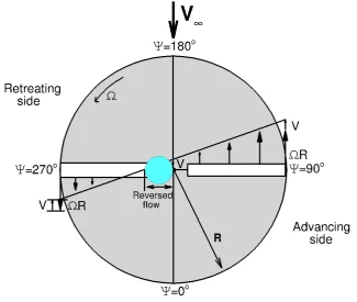
aircraft the flow field where the rotor operates is more complex and it is well described by Seddon[1]. In level forward flight the rotor is edgewise on to the airstream, a basically unnatural state for propeller

functioning. Practical complications which arise from this have been resolved by the introduction of

mechanical devices, the functioning of which in turn adds to the complexity of the aerodynamics. Fig.

1.1 presents the rotor disk as seen from above. The blade is rotating counter-clockwise with a rotational

speedΩ. The forward flight velocity isV, the radius of the blade isR, and the ratioV/ΩRis known

as the advance ratioµ of the rotor. The value ofµis normally between zero and 0.5. Azimuth angle

Ψis measured from the back of the disk, and the advancing side is defined for 0<Ψ<180, while the

retreating side is for 180<Ψ<360. In Fig. 1.1 the blade is shown atΨ=90oandΨ=270o. These

(28)

1.1. BACKGROUND-MOTIVATION CHAPTER 1. INTRODUCTION

rotating at fixed collective then much more lift would be generated on the advancing side than on the

retreating side. The consequences of this imbalance would be large oscillatory bending stresses at the

blade roots and a large rolling moment on the helicopter. Both structurally and dynamically the

rotor-craft would be unable to fly. As a result an azimuthal variation in blade incidence is needed to balance

lift on the two sides. This is achieved with the flapping hinges which allow the blade to flap up and down

during rotation. Thus as the blade moves on to the advancing side, the rise in relative velocity increases

the lift, causing the blade to flap upwards. This motion reduces the effective blade incidence thereby

reducing the lift and ultimately allowing the blade to flap down again. On the retreating side the reverse

process occurs. The fore and aft sectors now carry the main lift load. The total lift can also be restored

by altering the collective around the azimuth, but as this is done, the retreating blade, producing lift at

[image:28.595.110.436.361.636.2]

relatively low airspeed, will stall.

(29)

CHAPTER 1. INTRODUCTION 1.1. BACKGROUND-MOTIVATION

Compressibility effects are now present both on the advancing side where the Mach number is

high and on the retreating side where lower Mach number is combined with high blade incidence. A

tendency for the retreating blade to stall in forward flight is inherent in all present-day helicopters and is

a major factor in limiting their forward speed. Just as the stall of an airplane wing limits the low speed

possibilities of the airplane, the stall of a rotor blade limits the high speed potential of a helicopter.

Upon entry into blade stall, the first effect is generally a noticeable vibration of the helicopter.

This is followed by a rolling tendency and a tendency for the nose to pitch up. The tendency to pitch up

may be relatively insignificant for helicopters with semirigid rotor systems due to pendular action. If the

cyclic stick is held forward and collective pitch is not reduced or is increased, this condition becomes

aggravated; the vibration greatly increases, and control may be lost. The major warnings of approaching

retreating blade stall conditions are:

-Abnormal vibration

-Pitch-up of the nose

-Tendency for the helicopter to roll in the direction of the stalled side.

At high forward airspeeds, the following conditions are most likely to produce blade stall:

-High blade loading (high gross weight)

-Low rotor RPM

-High density altitude

-Steep or abrupt turns

Nowadays, the expectations for more efficient military and civil rotorcraft which will be faster,

easier to control and invisible are very high. To achieve these goals emphasis has been placed on control

of the flow around the rotor for aerodynamic enhancement, vibration decrease and noise elimination.

Modern flow control has a great influence on every major area of aeronautic engineering such as

ex-ternal aerodynamic enhancement, inex-ternal flows through propulsion engines, aero-acoustics and control

of turbulence. The ability to change the flow behaviour to a great extent, while a small amount of

(30)

characteristics of the flow is necessary to control it.

Referring to Gad-El-Hak[2], to choose a specific type of flow control, the presence or lack of wall, the Reynolds number, the Mach number and the flow instabilities should be taken into consideration.

The interrelation between different control goals shows that engineers have to make compromises to

achieve at least some of the goals. The first way to classify a flow control method is by indicating

whether the control is applied at the wall or away from it. Parameters such as wall surface, temperature,

mass transfer, suction or injection, different additives and control devices are some examples which can

influence the flow. A second classification has to do with the energy expenditure and the control loop

involved. There is passive control which needs no power and no control loop, and active control which

requires energy expenditure. As far as the active control goes, it is further divided into predetermined

and reactive. The predetermined control is not affected by the particular state of flow and requires no

sensors, while in reactive control the input is always adjusted based on some measurements. Reactive

control can be either feed-forward or feedback. Reactive feedback is classified into four categories:

adaptive, physical model based, dynamical-systems based, and optimal control.

At this section, the current state of art considering flow control devices for helicopter rotors will

be presented after the compilation of a literature survey. For this survey several databases and keywords

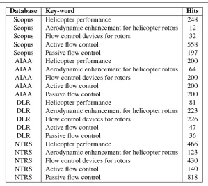
were used. The results for each of them are presented in Table 1.1. The search was based on keywords

found in the title as well as the abstracts of the publications, which justify the total number of the results.

In addition these keywords were always combined with the "fluid dynamics" keyword. After removing

the irrelevant papers and focusing on the research done the last twenty years the results found were

considerably decreased.

From this survey it is pointed out that the variety of flow control devices can be classified into

two categories. The first contains fluidic mechanisms that try to change the flow behaviour by adding

or removing momentum where is needed. Surface blowing circulation control, surface suction devices,

jets vortex generators, synthetic jets and plasma technology are such devices. On the other hand, there

are devices which do not affect directly the flow characteristics, but they contribute to the control of the

(31)

[image:31.595.153.462.113.374.2]

CHAPTER 1. INTRODUCTION 1.1. BACKGROUND-MOTIVATION

Figure 1.2: Classification of flow control strategies[2].

Gurney flaps are common mechanisms of this second category. However, the way these devices are used

and their effectiveness on flow control is strongly related with the specific target of the control. That may

be the delay of flow separation caused by dynamic stall or BVI or even the blade vibration decrease,

and noise diminution. Another significant factor which is considered when choosing the appropriate

device is the type of control, as classified above by Gad-El-Hak[2], the energy that will be consumed and the load penalty. These characteristics make flow control a demanding and challenging process which,

however, has the potential to improve aerodynamic performance and extend the capabilities of current

rotor systems. Figure 1.3 presents the interrelation between flow control objectives to give an idea of

how strongly they are connected.

The target of this research is the investigation of the potentials and limitations of flow control

devices and the suggestion of an innovative flow control mechanism for helicopter rotor. As this

(32)

Database Key-word Hits

Scopus Helicopter performance 248 Scopus Aerodynamic enhancement for helicopter rotors 12 Scopus Flow control devices for rotors 32 Scopus Active flow control 558 Scopus Passive flow control 197 AIAA Helicopter performance 200 AIAA Aerodynamic enhancement for helicopter rotors 64 AIAA Flow control devices for rotors 200

AIAA Active flow control 200

AIAA Passive flow control 200

DLR Helicopter performance 81 DLR Aerodynamic enhancement for helicopter rotors 223 DLR Flow control devices for rotors 226

DLR Active flow control 47

DLR Passive flow control 36

NTRS Helicopter performance 466 NTRS Aerodynamic enhancement for helicopter rotors 123 NTRS Flow control devices for rotors 430

NTRS Active flow control 140

[image:32.595.126.426.82.350.2]

NTRS Passive flow control 818

Table 1.1: Databases results for literature survey.

control devices were used in the past twenty years until present and to analyse their effects in the

be-haviour of the flow. All flow control devices analysed here were found to offer substantial benefits to the

performance of the rotors. There are, however, difficulties regarding the efficient simulation of these

de-vices using CFD. The most important issue identified were the large differences in spatial and temporal

flow scales that had to be modelled.

Considering the performance of a helicopter, the weight-speed envelope faces limitations due to

the advancing blade restricting speed and due to the retreating blade stall restricting weight. In order

to minimise these limitations, drag should be decreased and pitching moment should be controlled at

the advancing side, while maximum lift without stall should be achieved at the retreating side. As a

result, flow control devices must affect these requirements in order to be suitable for rotor application.

According to Bousman’s Dynamic stall function [3]_{presented in Figure 1.4 at the end of this survey}

the flow control mechanisms will be classified in terms of increase of lift coefficient and decrease of

(33)

[image:33.595.133.524.133.539.2]

CHAPTER 1. INTRODUCTION 1.2. FLUIDIC DEVICES

Figure 1.3: Interrelation between flow control goals[2].

1.2 Fluidic devices

1.2.1 Vortex Generators

(34)

[image:34.595.101.449.81.360.2]

pro-1.2. FLUIDIC DEVICES CHAPTER 1. INTRODUCTION

Figure 1.4: Optimising for dynamic stall control - Bousman’s dynamic stall function[3]. duced by the VGs. Fluid particles with high momentum in the streamwise direction mix with the low

momentum viscous flow inside the boundary layer, thereby, the mean streamwise momentum of the

fluid particles in the boundary-layer is increased. The process provides a continuous source of

momen-tum to counter the natural boundary-layer momenmomen-tum decrease and the growth of its thickness caused

by viscous friction and adverse pressure gradients. Vortex generators can reduce or eliminate flow

sepa-ration in moderate adverse pressure gradient environments. Even when sepasepa-ration does occur for cases

of large adverse pressure gradient, the mixing action of trailing vortices will restrict the reversed flow

region in the shear layer and help maintain some pressure recovery along the separated flow. Thus the

effects of separation may be localised or minimised.

The concept of micro vortex generators was most probably first introduced by Keuthe in the

1970s[5]_{. In his work, wave-type micro VG with height of 27% and 42% of the boundary layer thickness}

were installed on an aerofoil to reduce trailing edge noise by suppressing the formation of a Karman

vortex street and by reducing the velocity deficit in the aerofoil wake. Since the late 1980s, these devices

(35)

submerged vortex generator[7], low-profile vortex generator[8]and micro vortex generator[9].

The main difference between the SBVG and the VG is in terms of the device height. In general,

the velocity deficit within a turbulent boundary layer is dominant near the wall within the inner 20% of

the boundary layer thickness. In that region, an adverse external pressure gradient tends to lower the

ve-locity and thus promotes flow separation. Although both devices operate based on a similar mechanism

(generation of streamwise vortex), there are some major differences. For example, the SBVG produces

a larger velocity gradient close to the wall and has a stronger and lower deficit region in the profile. A

vortex generator achieves boundary-layer control only at the penalty of possible considerable drag. A

sub-boundary vortex generator produces vortices that travel downstream along the surface, causing flow

mixing between the inner layers of the boundary layer. Although these SBVGs will produce extra drag

as compared with a clean surface, their drag penalty is less than with VGs.

The wide range of conditions where the rotor is operating at makes the parasitic drag a

partic-ular limitation, which consists the main drawback of VGs. The only way to avoid this problem is the

use of sub-boundary layer VGs as they remain within the low energy flow in the boundary layer and

consequently they have low drag. On the other hand, Linet al.[9][10]used SBVGs on a multi-element aerofoil in a landing configuration and showed that VGs as small as 0.18% of reference wing chord

can effectively reduce boundary layer separation on the flap which will lead to reduction of drag and

increase of lift for a given angle of attack. In fact during his experimental study trapezoidal vanes were

placed on the 25% of the chord of the flap of a wing at flow conditions M=0.2 andRe=5×106_creating

counter-rotating vortices, and they achieved a 10% lift increase, 50% drag decrease and 100% increase

of L/D ratio.

As stated in Kenning’s review[11]_{the potential applications of VGs and SBVGs include control}

of leading edge separation, shock induced separation and smooth surface separation. SBVGs have less

parasitic drag but in case of shock induced separation they must be located closer to the separation line

which may be a major limitation in the unsteady application of the rotorcraft. Sub-boundary vortex

(36)

1.2. FLUIDIC DEVICES CHAPTER 1. INTRODUCTION

of SBVGs is linked with local boundary thickness which dependents on Reynolds number and angle

of incidence. Ashill et al. [13] also performed a separation control experiment where separation was introduced by placing a bump in the test section. The turbulent boundary layer tunnel was used with a

free stream velocity of 40m/sand a boundary layer thickness of 40mmover the bump. Three types of

SBVGs including the micro ramp, micro vane and split micro vane (with a gapg=1h) were tested. All

the devices had the same height ofh=10mm, resulting in a height ratio ofh/δ =0.25. Laser Doppler

anemometry (LDA) was used to perform velocity measurement in streamwise and lateral planes. The

velocity fields revealed a significant reduction of the separation region at the rear of the bump for all

three devices, furthermore it was found that the split micro vane yielded the best results.

Figure 1.5: Array of counter rotating triangular vortex generators[10].

1.2.2 Air-Jet Vortex Generators

Flow separation is a complex phenomenon influenced by a combination of factors, of which adverse

pressure gradients play a significant role. Adverse pressure gradients may reduce the relative motion

between the various fluid particles within the boundary layer. If this relative motion is reduced to a

sufficient level, the boundary layer can separate from the surface. Furnishing the boundary layer with

additional momentum may allow greater penetration against adverse pressure gradients with a reduction

in the magnitude of flow separation. Generating a series of longitudinal vortices over the surface of

(37)

to the near wall region provides the boundary layer with additional momentum. The presence of a

series of vortices again promotes such behaviour. An alternative to vane vortex generators is an active

fluid jet vortex generator. The first practical application of the technique is attributed to Wallis. Fluid

injection via inclined and skewed wall-bounded jets act to induce longitudinal vortices for flow control,

instead of solid vane vortex generators. Air jet vortex generators usually consist of an array of small

orifices embedded in a surface and supplied by a pressurised air source, wherein longitudinal vortices

are induced by the interaction between the jets issuing from each orifice and a free-stream fluid flow. The

orifices are pitched at angleΦwith respect to the surface tangent and skewed at angleΨwith respect to

free-stream flow. Prior studies have highlighted the advantages of carefully selecting parameters such as

the pitch and skew of the jet axis, as well as the orientation and the preference of certain orifice shapes.

Freestone performed a study at low speeds and identified that the optimum jet orientation for maximum

vorticity generation was a pitch angle of 30 deg and a skew angle of 60 deg. With this orientation

the resulting vortex strength could match and, in some cases, exceed that generated by an equivalent

vane vortex generator. Princeet al.[14, 15] compared the effectiveness of passive and active blowing over a NACA 23012 and a NACA 632−217 and showed that by comparing the ratioCL/(CD+CM) it is obvious that active AJVGs are more effective than passive ones only at highest angles of attack.

Moreover, a very important factor for the passive system is the pressure difference between the

air-jet intake and exit which drives the flow through the duct. For that reason Krzysiak proposed to use

the aerofoil overpressure regions as a source of the air for the AJVGs. These self-supplying air-jet

vortex generators are characterised by the fact that they remain inactive at low angles of attack and

only become active at higher angles of attack, close to critical values, as a result of the greater pressure

difference between the upper and the lower aerofoil surfaces. However, although this type of AJVG

is technically significantly simpler than the conventional one it works well, and delays separation only

for Mach number up to 0.4, but for higher speeds its influence deteriorates. Shunet al.[16] _studied

experimentally the exponential injection scheme firstly introduced by Eroglu and Breidenthal over a

NACA 63-421 aerofoil. The exponential jet appears to be a promising device for separation control as

(38)

a given factor ofe(2.71828) and a fluid injection velocity profile that also increases by the same given

factor. The experiment showed that the exponential jet produces worthwhile performance gains and an

increase in energy efficiency. In many cases it was found that the conventional vortex generators could

be successfully replaced by the air-jet vortex generators for boundary-layer control because of the ease

of control accompanied by a minimal drag penalty[14]. However, the complexity of the installation of AJVGs in comparison with the simplicity of the vane vortex generators has limited their practical usage.

The identification of the optimum air-jet configuration is not simple and needs careful study, because

the effectiveness of AJVGs depends on a number of parameters such as the pitch and skew angles,

the jet mass-flow rate, the ratio of the boundary-layer thickness to the jet diameter, the jet Reynolds

number, and the ratio of mean jet velocity to mean free-stream velocity. In addition, using active or

passive blowing depends on the energy required and its source such as the engine of the helicopter in

which intake air can be bled away to feed the jets. In this case, the system will result in a small loss

in engine efficiency, equivalent to an increase in parasitic drag which must be taken into consideration

when calculating the overall efficiency of AJVGs. A research that could lead to useful conclusions

concerning the application of AJVGs in helicopter rotors is conducted by Singhet al.[17]. In that study two arrays of AJVGs were located at x/c=0.12 and x/c=0.62 on an oscillating RAE 9645 aerofoil. The

effect of operating only the one or both of the arrays, as well as the influence of blowing rate were

investigated and the results showed that blowing from the front array atC_µ=0.01 is more effective than

blowing either from the rear array or from both arrays simultaneously. However this work is restricted

to low-speed dynamic stall. For most helicopters the retreating blade operates at Mach number of about

0.4, which means that the blowing requirements may increase under these conditions and the optimum

location of the arrays may also change. Furthermore, the sensitivity of AJVG at real rotor effects such

as flow skew angle, radial flow, and time-varying Mach number may also be an issue. Finally, if the

(39)

1.2.3 Synthetic Jets

Synthetic jets consist of a vibrating diaphragm at the base of a small cavity just under the aerofoil

surface. The diaphragm is activated electrostatically or through the use of a piezoelectric material with

frequencies that span 1-14 kHz. A small hole through the surface allows the production of a stream of

ring vortices travelling out from the surface as shown in the schematic.

Hassanet al.[18][19]_{showed by numerical study that zero-net-mass jets can, with careful selection}

of their peak amplitude and oscillation frequency, enhance the lift characteristics of aerofoils. Indeed, a

NACA0012 was used at a free-stream Mach number of 0.6 and Reynolds numberRe=3x106and for jet velocities 0.05, 0.1 and 0.2. It is shown that as the jet velocity is increased the lift is increase while

the moment and drag are decreased. As far as rotor blades is concerned two arrays of synthetic jets

can be used to change the local pressure distribution near the leading edge resulting in lower temporal

pressure gradients and lower Blade Vortex Interaction noise levels. The effectiveness of these devices

for lift enhancement increases with the increase of free-stream Mach number and the decrease of the

ratio between the jet Mach number and free-stream Mach number. When comparing synthetic jets with

AJVGs the advantage is that it is easier to provide power rather than air. On the other hand, researchers

must always keep in mind that the implementation of any device will be pointless if the power needed

exceeds the power gained by controlling the flow.

1.2.4 Surface Blowing Circulation

Blowing air tangentially to the aerofoil surface has been employed both at leading and trailing edges

of the wings. Park[20]_{showed that in the case of uniform blowing from a slot, the skin friction on the}

slot rapidly increased. The near wall stream-wise vortices were lifted up by blowing, and as a result the

interaction of the vortices with the wall became weaker. Moreover, the lifted vortices became stronger in

the downstream due to less viscous diffusion above the slot and more tilting and stretching downstream

of the slot, resulting in the increase of the turbulence intensities as well as the skin friction downstream

(40)

which has been tested in the Army’s water tunnel at NASA Ames Research Centre in the early 1980s.

The aerofoil was oscillating with a pitching motion of α =10deg+10deg x sin(2πf t), a reduced

frequencykof 0.49, and a Reynolds number of 30,000. The tangential blowing slot was located at the

quarter chord on the upper surface of the aerofoil. Three blowing rates were tested. Without blowing

(C_µ =0.0) the aerofoil stall at 13 deg. For the case of injection at twice the free-stream velocity the

blowing delays the stall until about 25 deg. and shows a moderate amount of increase in lift. For the

third case where the injection was four times the free-stream velocity there is no sign of stall even at 30

deg, while the lift is higher compared to the second case. Again the power losses related to a blowing

system are difficult to estimate without undertaking a full rotorcraft design study. The experimental

results show that the upper-surface blowing concept delays the dynamic stall phenomenon by trapping

the stall vortex. Further study with the computational method indicates that a stall vortex does not form

on the airfoil when there is upper-surface blowing at the quarter chord. Although the concept seems

to have some effectiveness in delaying dynamic stall, the application of these concepts to rotorcraft

requires further tests on the effects of high Mach numbers and high Reynolds numbers.

Mitchellet al.[22] of ONERA also used blowing circulation as a method to control the vortex breakdown location. In general the vortex breakdown phenomenon can be characterised by a rapid

deceleration of both the axial and swirl components of the mean velocity and, at the same time, a

dramatic expansion of the vortex core. The no-blowing configurationC_l=0 of the delta wing was

examined for U=15, 24, and 40 m/s at a=20, 27, 30, and 40 deg. The Reynolds numbers associated with

each U are, respectively,Rec=9.75x105, 1.56x106, and 2.6x106. Open-loop, asymmetric, blowing along the core of the port-side leading-edge vortex on the leeward surface of the delta wing was shown

to be effective for controlling the vortex breakdown-location over the delta wing.

1.2.5 Surface Suction

In the case of highly manoeuvrable aircraft like helicopters, suction technique can be applied to delay

stall by delaying the detachment of stall vortex and taking advantage of the increased dynamic lift. The

(41)

a NACA0012 by removing the reverse-flowing fluid at the same rate as it arrives in the leading-edge

region. It is shown that the pitch rate of the aerofoil is the main factor that influences the suction

requirements and when this rate is low the Reynolds number becomes significant as the transition of

turbulence in the shear layer makes the flow more complex. The location of the slot used for the suction

is less important, as long as it is the area where the reverse-flowing fluid can be removed and when the

suction is applied in a uniform way it requires less velocity and therefore energy rather than when it is

applied in a concentrated way. As far as the suction activation goes, this should happen before the angle

at which the shear layer lift-up takes place and the control should be continued as long as it is desired as

if its termination before the right time will lead to an immediate formation of the dynamic-stall vortex.

Badramet al.[24]_{and Lorber}_{et al.}[25]_{investigated the effect of suction on the wing surface on vortex}

break-down with leading-edge suction and surface suction. In first the case suction was found to be more

effective in delaying vortex breakdown for suction slits closer to the leading edge. On the other side, the

exact mechanism of how the surface suction affects the vortex breakdown was not clear. Surface suction

is also being studied as a means to reduce viscous drag by delaying laminar to turbulent boundary layer

transition, but as a conclusion surface suction is less effective than leading-edge suction.

1.2.6 Plasma technology

The last few years researchers[26],[27],[28],[29] have focused on Plasma technology for enhancing the flow around aerofoils and wings. Caruanaet al.[30]describes the plasma technology and its applications on aerodynamic control for civil aircraft as part of PLASMAERO project. The technology of plasma

can be classified into the family of the active means of control. The advantages of using plasma are

located at the fact that their use can be of a big simplicity, their high frequency of functioning will allow

a real-time control, their consumption of electric energy is reduced and no pneumatic circuit is useful.

According to Post[31]_{the main advantages of Plasma are:}

1) They are fully electronic with no mechanical parts and, therefore, are able to withstand high force

loading.

Flow control on helicopter rotors using active gurney flaps