Optimisation of aspects of rotor blades using computational fluid dynamics

(1)

Optimisation of Aspects of Rotor Blades using Computational Fluid Dynamics

Thesis submitted in accordance with the requirements of the University of Liverpool for the degree of Doctor of Philosophy

by

Catherine Johnson

(2)

(3)

Declaration

I hereby declare that this dissertation is a record of work carried out in the School of Engi-neering at the University of Liverpool during the period from November 2008 to June 2012. The dissertation is original in content except where otherwise indicated.

June 2012

...

(4)

Abstract

(5)

List of Publications

In Journals

• C.S. Johnson and G.N. Barakos, A Framework for Optimising Aspects of Rotor Blades, The Aeronautical Journal, vol.115, Issue 1165, p.147-161,15p, March 2011.

• C.S. Johnson, M. Woodgate and G.N. Barakos, Optimisation of Aspects of Rotor Blades in Forward Flight, International Journal of Engineering Systems Modelling and Simulation, vol.4, Issue 1/2, p.79-93, 2012.

• C.S. Johnson and G.N. Barakos, Development and Demonstration of a Framework for Op-timising Aspects of Rotor Blades in Forward Flight, International Journal for Numerical Methods in Fluids (in review)

In Conference Proceedings

• C.S. Johnson and G.N. Barakos, Development of a Framework for Optimising Aspects of Rotor Blades, American Helicopter Society 66th Forum, Paper 377 [CDROM], Phoenix, Arizona, May 2010.

• C.S. Johnson and G.N. Barakos, Optimising Aspects of Rotor Blades in Forward Flight, AIAA Forum, Paper ID 895432, Orlando, Florida, USA, Jan 2011.

• C.S. Johnson and G.N. Barakos, Rotor Tip Optimisation in Forward Flight, 46th Sympo-sium of Applied Aerodynamics, Aerodynamics of Rotating Bodies, Paper 32 in Conference Proceedings, Orl´eans, France, March 2011.

• C.S. Johnson and G.N. Barakos, Optimisation of Aspects of Helicopter Rotor Blades and Fuselage, 37th European Rotorcraft Forum, Paper 93, Milan, Italy, 13-15th September 2011.

Technical Notes

• Technical Note, TN10-013, Parameteric Mesh Generation for HMB.

(6)

Acknowledgements

I would like to thank my supervisor, Prof. George Barakos for being an exemplary mentor and a brilliant advisor for this project. His passion for research and his experiences have taught me a lot that I won’t forget. I would also like to thank Dr. Steijl and Dr. Woodgate for their consis-tent support throughout the period of this project. I deﬁnitely could not have achieved so much without them. Thank you to my work colleagues who have also been a great support in and out the lab, both those present now and those who were here previously. I have enjoyed working with this group of people because of the quality of work produced and the diversity and character of the people that make it. I would also like to mention Alan Brocklehurst and thank him for his valuable advice and for his time. I learnt much from him in every conversation.

In addition, I would also like to thank my family who have been my unconditional support in every aspect. I would like to honour my father who is an inspiration to me and has sacrificed much for me in this time. A very special thank you goes to my sister and greatest friend, Caro-line, for being my ever present help in times of need regardless of what it may be, even learning about my project with me. I’d like to also thank Sidra, my housemate, who also recently finished her PhD. It was great to have her as a friend on this journey from the first day as engineering undergraduates to the last day as PhD students.

(7)

List of Figures

1.1 (a) General design process for helicopters, (b) The design process involving rotors. (Cour-tesy of Stanley A. Orr and Robert P. Narducci, Framework for Multidisciplinary Analysis, Design, and Optimization With High-Fidelity Analysis Tools, NASA/CR-2009-215563, Feb

20091). . . . 6

1.2 Various blade planform proﬁles. . . . 7

1.3 Figure showing power as a function of velocity of forward ﬂight2_{. . . .} ₁₅

1.4 Figure comparing blades optimised for diﬀerent objectives. . . . 15

1.5 Figure showing how the gradient-based optimiser, CONMIN operates. Three points, A,B and C are shown in various locations with regard to the constraints. At A, steepest descent is used to reach the minimum, at B, a constraint is encountered and the point attempts to move along the constraint contour and at C, the point attempts to overcome the constraint.3 ₁₆ 1.6 Comparison of the methods used in optimisation techniques developed in the last 50 years. It can be seen that ranking, Pareto and weights are the techniques that have become most popular.4 _{. . . .} ₂₄

1.7 PARSEC variables of an aerofoil for parameterisation5_. _{. . . .} ₂₉

2.1 Pressure contours of the UH60 rotor using 2 and 4 modes for the Harmonic Balance method (red lines) compared to the solution from the time-marching method (black lines). The lines represent isobars at the same pressure values at an azimuth of 90 degrees, which represents the worst case. . . . 38

2.2 Experimental data in comparison to CFD by time marching (TM) and Harmonic Balance (HB) methods. The mean value has been removed. . . . 39

2.3 C grid for aerofoils. . . . 39

2.4 Grid for hovering rotor. . . . 40

3.1 Map of the processes involved in the optimisation of rotors. . . . 43

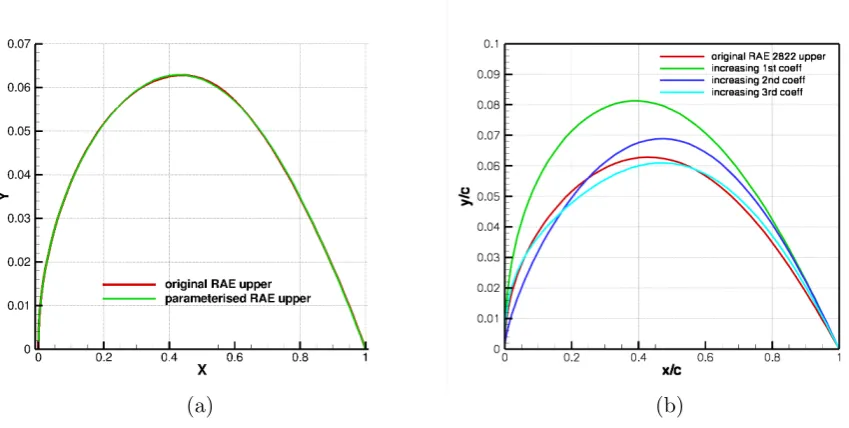
3.2 (a) The original upper curve compared to the parameterised upper curve of the RAE 2822. Error convergence was 0.0074. (b)The effect of increasing the 3 coefficient values to the upper surface curve. The original surface’s six coefficients are α1 = 0.009149, α2 = 0.001444, α3=−0.000325,α4=−0.000266,α5=−0.000060,α6=−0.000050. . . 47

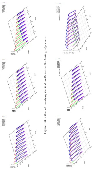
3.3 Effect of modifying the first coefficient to the leading edge curve. . . . 48

3.4 Effect of modifying the first and second coefficients to the leading edge curve. . . . 48

3.5 Eﬀect of modifying the third and fourth coeﬃcients to the leading edge curve. . . . 49

3.6 Eﬀect of adding more coeﬃcients to the leading edge curve. . . . 49

3.7 BERP-like tip Schematic. . . . 51

3.8 (a) Notch gradient, (b) sweep and (c) delta parameter equation deﬁnitions for the BERP planform. . . . 51

3.9 ROBIN fuselage with additional parts. . . . 52

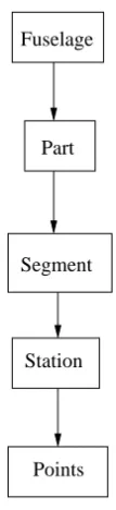
3.10 Fuselage Parameterisation hierarchy. . . . 53

3.11 Example of parts of a fuselage created using the parameterisation method. . . . 54

3.12 Schematic of the mesh generation process. . . . 54

3.13 An example of a neural network trained to receive inputs such as camber and thickness to obtain the lift coeﬃcient (adapted from Spentzos6). . . . 57

(11)

3.15 Error convergence comparison for an example ANN. This is for the optimisation of a NACA 5-digit rotor section on a blade in forward flight. The x-axis is the camber value of the section and the y-axis is the peak-to-peak moment of the section over a full revolution. The various curves and the legend correspond to the training of the ANN to converge at different error values as well as a comparison with the ANN that had an adaptive learning rate. The black dots represent the data used for training and the pink dots are the accurate CFD data not used in the training set. i.e. validation data. The full test case analysis can be found in Chapter 5. . . . 60 3.16 Comparison of ANN prediction for scaled average C_l, C_dand Cmwith different numbers of

outputs (out), hidden layers (hl) and neurons (n). The number of inputs is constant at two. This is for the optimisation of a NACA 5-digit rotor section on a blade in forward ﬂight. The x-axis is the camber value of the section and the y-axis is the average moment, lift and drag of the section over a full revolution. The various curves and the legend correspond to the training of the ANN with diﬀerent numbers of neurons and layer. The black dots represent the data used for training and the cyan dots are the accurate CFD data not used in the training set. i.e. validation data. The full test case analysis can be found in Chapter 5. 61 3.17 Comparison of ANN prediction accuracy with polynomial of order 4 and 10 for ∆C_m. 3

hidden layers (hl) and 15 neurons (n) were used for the ANN. Number of inputs is kept constant at 2. The solver training and prediction comparison is included. . . . 63 3.18 Comparison of ANN prediction accuracy with polynomial of order 10 and kriging for∆C_m.

3 hidden layers (hl) and 15 neurons (n) were used for the ANN. Number of inputs is kept constant at 2. The solver training and prediction comparison is included. ON the right, the blue surface is the ANN prediction and the red is the kriging prediction. . . . 65 3.19 Comparison of ANN prediction and POD prediction trained with the original database of

20 CFD points less the two that are predicted. . . . 68 3.20 Comparison of original data (ANN predictions of average Cm for varying NACA aerofoil

thicknesses at R =50% - see Chapter5) with POD interpolation predictions comparing number and position of training data points. . . . 68 3.21 Outline of the genetic algorithm employed for an aerofoil selection case and the analogy

with genetics.. . . 69 3.22 Pareto front and objective function type optimisers. . . . 71

4.1 Cp plots predicted by XFOIL for the parameterised aerofoil NACA 23009 (a) and the

original NACA 23009 aerofoil (b) at Mach 0.2 and Re = 1×106_. _{. . . .} ₇₃ 4.2 Cp plots predicted by XFOILfor the parameterised ONERA aerofoil OA 213 (a) and the

original ONERA aerofoil OA 213 (b) at Mach 0.2 and Re = 1×106_{. The error convergence}

was about 0.03 resulting in large diﬀerences in moments especially. This suggest a smaller error is required and hence a value of 0.01 was chosen. . . . 73 4.3 Cp and aerofoil section comparison of the original and parameterised RAE 2822 at Mach

= 0.725 and AoA = 2.92 degrees. . . . 75 4.4 C_l/C_dANN predictions of varying 1st3 coeﬃcients of parameterised upper surface of RAE

2822. Optimum seems to aim for lowα1andα2and highα3. No constraints are implemented. 76 4.5 Mach number contours and C_p for (a) the original RAE2822 aerofoil, (b) and (c) the

optimised aerofoils in Table 4.2. Free stream Mach number = 0.725, AoA = 2.92o, Re = 6.5×10-6. . . . 77 4.6 The original RAE 2822 and the optimised aerofoil shape: α1 - 7.95×10-4,α2+ 1.34×10-4,

α3+ 3.006×10-3. . . . 78 4.7 Pareto front for the RAE 2822 aerofoil using drag divergence Mach number, C_l and C_d.

The grey surface is a surface plot of these values. The black dots make up the Pareto front points and the blue spots are the GA’s selection using the objective function. . . . 78 4.8 LHS comparison for the RAE 2822 moment coeﬃcient. . . . 79

(12)

5.2 C_d for varying NACA aerofoil camber - thickness 9, 12, 15 and 18% chord at the inboard

station, r/R = 0.5. M_loc= 0.35, M_∞ = 0.2 in forward ﬂight. . . . 82

5.3 C_dfor varying NACA aerofoil camber - thickness 9, 12, 15 and 18% chord at the outboard station, R = 90%. M_loc= 0.63, M_∞ = 0.2 in forward ﬂight.. . . 83

5.4 C_mfor varying NACA aerofoil camber - thickness 9, 12, 15 and 18% chord at the inboard station, R = 50%. M_loc= 0.35, M_∞ = 0.2 in forward ﬂight.. . . 83

5.5 Cmfor varying NACA aerofoil camber - thickness 9, 12, 15 and 18% chord at the outboard station, R = 90%. M_loc= 0.63, M_∞ = 0.2 in forward ﬂight.. . . 84

5.6 C_l for varying NACA aerofoil camber - thickness 9, 12, 15 and 18% chord at the inboard station, R = 50%. M_loc= 0.35, M_∞ = 0.2 in forward ﬂight.. . . 84

5.7 C_lfor varying NACA aerofoil camber - thickness 9, 12, 15 and 18% chord at the outboard station, R = 90%. M_loc= 0.63, M_∞ = 0.2 in forward ﬂight.. . . 85

5.8 Pressure contours on the lower and upper surface of NACA 0015 for increasing azimuth angle. R = 90%, M_r/Rin hover would be 0.63 and M_∞= 0.2 in forward ﬂight. . . . 85

5.9 Variation of loads for r/R = 50% and 90%; Red represents the upper extreme and blue, the lower extreme. . . . 87

5.10 Comparison for the dM/dt cases inboard, midboard and outboard stations of the use of pareto optimisation, objective functions and both i.e. objective function used for selection pressure on designs. . . . 88

5.11 Comparison of the optimum surface created by the ANN (blue) and Kriging (red) meta-models. The GA selection is shown as white dots. . . . 89

6.1 Deﬁnition of the parameters for optimisation of the wing. . . . 91

6.2 Grid for the wing. . . . 91

6.3 LHS comparison for the near laminar ﬂow wing elliptic loading. . . . 92

6.4 ANN (black) and Kriging (white) comparison for the wing optimisation performance pa-rameter, E_ell. . . . 92

6.5 ANN prediction using CFD training data (black dots) for M1 and M2 values, shown at 0 ∆M1 and ∆M2. . . 93

6.6 ANN predictions of performance parameters as a function of the position of chord variables. 94 6.7 The average ﬁtness per generation. Note that, here the OFV is minimised. . . . 95

6.8 GA selection of ANN prediction of L/D and elliptic loading.. . . 95

6.9 Planform comparison of the designs in Table 6.1. . . . 96

6.10 Comparison of velocity magnitude contours for the optimised blade (red) and the original blade (black) at 2.3 chord lengths behind the trailing edge. . . . 96

6.11 Cpdistribution of the designs in Table 6.1 and secondary ﬂow visualisation a chord length behind the trailing edge. The green points are for the rectangular blade and are shown as a reference. . . . 97

6.12 C_L distribution visualisation using velocity magnitude (left), and streamline visualisation of secondary ﬂow (right) at 2.5 chord lengths behind the trailing edge for the wings in Table 6.1. . . . 98

6.13 Q criterion iso-surface =1×10−6 _{showing extent of vortex tip.} _{. . . .} ₉₉

7.1 Rotor in hover, Aspect Ratio = 16, Coning = 0, Anhedral = 0, Twist = 0, 8 and 12o: FM, C_T and C_Qvs collective angle. M_tip= 0.6. . . . 101

7.2 ANN predictions of (a) FM vs C_T and (b) C_T vs. C_Q for 5 values of collective used to train the ANNs. . . . 102

7.3 Rotor in hover, Aspect Ratio = 16, Coning = 0, Anhedral = 0, Collective = 12oand various twist distributions at the root and tip. M_tip= 0.6. . . . 103

7.4 ANN and kriging predictions and validation for FM. . . . 105

7.5 ANN predictions of (a)F Mmax vs. twist and (b)∇F M vs. twist.. . . 105

7.6 GA selection of optimum twist based on the maximum FM and the change in FM with collective angle increase for 5 values of collective used to train the corresponding ANN. . . 106

(13)

7.8 Visualisation of tip vortices using Q criterion (value of 0.1) for a range of twists atθ = 12

degrees.. . . 108

7.9 LHS comparison for the FM of a rotor in hover. . . . 108

8.1 UH60 rotor blade twist and aerofoil distribution.. . . 109

8.2 UH60 optimisation for sweep, anhedral and twist CFD design points. . . . 111

8.3 UH60 tip geometry for sweep modiﬁcation. . . . 111

8.4 UH60 tip sweep geometry planform curvature. The black surface has a sweep of 10 degrees and the blue, a sweep of 40 degrees. . . . 112

8.5 Anhedral implementation using gradient matching between mid section and initiation section.113 8.6 Anhedral implementation for the UH60-A using a smoothed arc. . . . 113

8.7 Experimental data in comparison to CFD data by time marching (TM) and Harmonic Balance (HB). . . . 114

8.8 M2Cn(left) and M2Cm(right) plots for the UH60 with 20 deg sweep and increasing anhedral.116 8.9 M2C_n(left) and M2C_m(right) plots for the UH60 with diﬀerent sweep and 0 deg anhedral. 117 8.10 M2Cn(left) and M2Cm(right) plots for the UH60 with diﬀerent sweep and 15 deg anhedral as well as the original rotor. . . . 118

8.11 Total and vibratory pitching moments for a single blade over a revolution of the rotor in forward ﬂight. The original rotor has 20 degrees sweep and 0 degrees anhedral. . . . 119

8.12 ANN prediction for pitching moments of a blade with varying sweep and anhedral. Values were scaled with original blade of 0 deg anhedral, 20 deg sweep. Black dots on the plot are data used for training the ANN. GA selections are shown as red dots. . . . 121

8.13 (a) Genetic algorithm results, (b) Comparison between Pareto front optimisation and ob-jective function selection. . . . 121

8.14 Cp plots at diﬀerent azimuth angles for the original (SW20AN0) and validation point (SW17.1AN11) UH60 rotors at the swept part of the blade, where R = 15.5. . . . 122

8.15 ANN predictions of FMmaxand∇FM. . . . 123

8.16 (a) ANN prediction of the FM, (b) Optimum twist distribution for hover of the blade optimised for forward ﬂight. . . . 124

9.1 (a) Step 2 and (b) Step 3 of the mesh generation process demonstrated with the ROBIN body. . . . 126

9.2 JAXA JMRTS fuselage in the wind tunnel showing that the isolated fuselage data was obtained with the hub grips on7_. _{. . . 127}

9.3 JMRTS Fuselage C_p distribution along Y=0 (centerline). Freestream Mach number is 0.175, Reynold’s number is 1.1 million and the angle of attack is -2 degrees. The mesh size is about 3 million cells. . . . 128

9.4 Pressure distribution comparison between the original and the parameterised shape. Freestream Mach number is 0.175, Reynold’s number is 1.1 million and the angle of attack is -2 degrees.128 9.5 (a) The parts along the x-axis that make up the parameterised JAXA fuselage, (b) The fuselage grid position showing x coordinate deﬁnitions (this is translated compared to Figure 9.5(a) so that the rotor centre is at the origin). . . . 131

9.6 JMRTS fuselage shape comparison between parameterised original, coefficient C2 = 1.645 (red), one with coefficient C2 = 1.24 (white) and one with coefficient C2 = 2.0 (cyan). The C_L for all of these bodies was approximately 0.00012 to 0.00013. The C_D varied from approximately 0.0251 to 0.0267 and the C_M (about the origin which is where the hub is centred) was negligible (of the order of 10-5). . . . 134

9.7 Pressure distribution comparison of the parameterised fuselage with and without the actu-ator disk. C_T = 0.0047, µ= 0.16. . . . 135

9.8 Flow visualisation of separation occuring at the rear of the JMRTS fuselage. C_T= 0.0047, µ= 0.16,M_∞= 0.175.. . . 135

(14)

9.11 Cp distribution along the centreline for the parameterised and the modiﬁed JAXA bodies. 138

9.12 C_pdistribution differences along the fuselage of the original parameterised fuselage and the modified one (red is modified and blue is parameterised original). . . . 139 9.13 C_Pvariation for a selection of parameter values. . . . 140 9.14 Variation of drag coefficient for the front of the fuselage with change in parameterisation

coeﬃcient, C2. The original body has a parameterisation coeﬃcient of 1.645. . . . 140

9.15 Polar plot of the optimised and original showing Drag vs Angle of attack and Lift vs Drag coeﬃcient. The green curve is for the original and the red for the optimised. . . . 141

10.1 Vortex along the leading edge for the BERP tip8. . . . 143 10.2 (a) Cross section of the HH-02 and the NACA 64A-006 aerofoils used on this blade. The

baseline twist is 9 degrees linear. (b) the original planform of the BERP rotor obtained from Brocklehurst9. . . . 143 10.3 Planform view of the parameter changes to the geometry. . . . 144 10.4 Sample space for the planform of the BERP-like rotor. . . . 145 10.5 The value of the sweep parameter must be changed to with the notch position for the same

sweep. . . . 145 10.6 Visualisation of the three parameter changes to the blade tip geometry in ICEMCFD. . . 146 10.7 Schematic of the original fast ﬂying rotor blade used as an initial point for this optimisation

exercise. . . . 147 10.8 Eﬀect of twisting about the quarter chord point (top) or about the quarter chord line

(bottom).. . . 148 10.9 Anhedral deﬁnitions for the BERP tip.. . . 149 10.10Figure of Merit vs. thrust coeﬃcient of the original blade and the BERP variants with

varying twist and anhedral. . . . 150 10.11Lift distribution along the span with varying twist at 13 degrees of collective. . . . 150 10.12Aerofoil comparison to section on BERP-like rotor at the same conditions before the notch,

green is the 2D aerofoil and red is the rotor section, r/R = 0.75.. . . 151 10.13Aerofoil comparison to section on BERP-like rotor at the same conditions in the middle of

the notch, green is the 2D aerofoil and red is the rotor section, r/R = 0.862. . . . 151 10.14Aerofoil comparison to section on BERP-like rotor at the same conditions after the notch,

green is the 2D aerofoil and red is the rotor section, r/R = 0.918. . . . 151 10.15M2Cnfor the BERP-like rotors with ﬁxed parameters: NE = 11.5 and NE = 12, NG = 35

and variable sweep parameters. The black line indicates the M2C_n = 0 line. . . . 154 10.16M2Cm for the BERP-like rotors with ﬁxed parameters: NE = 11.5 and NE = 12, NG =

35 and variable sweep parameters. The black line indicates the M2Cm= 0 line. . . . 155

10.17M2C_qfor the BERP-like rotors with ﬁxed parameters: NE = 11.5 and NE = 12, NG = 35 and variable sweep parameters. The black line indicates the M2Cq= 0 line and the white

line indicates the approximate middle value, M2Cq= 0.2. . . . 156

10.18M2C_n, M2C_m and M2C_q for the BERP-like rotors with ﬁxed parameters: NG = 28 and variable sweep parameters for diﬀerent notch positions. Red is lowest sweep, blue is highest sweep. The arrow shows the freestream direction. . . . 157 10.19Comparison at azimuth 0, 90, 180 and 270 degrees of the M2C_n, M2C_m and M2C_q for

BERP-like rotor with ﬁxed parameters: NE = 11.5 and 12, NG = 28 and variable sweep parameters.. . . 158 10.20Comparisons of the integrated loads, M2C_m and M2C_q for BERP-like rotor with ﬁxed

parameters: NE = 11.5 and 12, NG = 35 and variable sweep parameters. . . . 160 10.21M2Cn, M2Cmand M2Cqfor the BERP-like rotors with ﬁxed parameters: NE = 11.75 and

SW = 0.21 with varying NG. The black line indicates a contour level = 0 line and the white line indicates the approximate middle value for M2Cq= 0.2. . . . 162

10.22M2Cmintegrated over the full blade at each azimuth for the BERP-like rotors. . . . 163

(15)

10.25The baseline BERP-like rotor in comparison to a swept tip design. The parameters for this rotor are NE = 12, NG = 25, SW = 0.25. . . . 165 10.26ANN predictions with training data and GA selection shown for each of the performance

parameters. The white dots are the GA optimal selection and the black dots are the CFD training data for the ANNs. The dashed line is where the contour level = 1 i.e. the value for the baseline design. . . . 165 10.27Pareto front points compared with GA selection; red is NE = 11.5, green is NE = 11.75,

blue is NE = 12. The white dots are the GA optimal selection and the cyan dots are the Pareto front solutions. . . . 165 10.28Pareto front for the BERP-like design. . . . 166 10.29(a) Pareto front points compared with GA selection; red is NE = 11.5, green is NE = 11.75,

blue is NE = 12, (b) OFV contour colour map in the design space. The white dots are the GA optimal selection, the cyan dots are the Pareto selection and the black dots are the CFD training data for the ANNs. . . . 166 10.30Optimum (red contour lines) compared to reference (black contour lines) for M2Cm and

M2Cq. . . . 167

10.313D view of load distribution for the optimum (red) and the original (blue) rotors. . . . 167 10.32OFV for the baseline and BERP-like rotor where the black contour lines represent the

reference rotor with parameters: NE = 12, NG = 25, SW = 0.25, and the red lines represent the optimised rotor with parameters: NE = 11.75, NG = 35 and SW = 0.21 where OFV=

−0.2×M2Cm−0.6×M2Cq. . . . 168 10.33Cpand planform distribution of the reference (blue) and optimised (red) BERP variant at

high thrust (collective = 13 degrees) in hover. . . . 168

B.1 (a)Imported points of aerofoils. (b) Points around the aerofoil to which vertices will be assosciated to. . . . 235 B.2 (a) Curves around the wing. (b) Surface around the wing. . . . 236 B.3 (a)Full ﬂow ﬁeld. (b) Blocking and points around the wing tip. . . . 236

C.1 ROBIN fuselage compare Cp with experimental data. Mach number = 0.062, Re = 3×10-6.249

C.2 ROBIN-mod7 fuselage Cp comparison from Schaeﬄer et al. at 0 degrees angle of attack

and Mach number 0.110 _{. . . 250}

C.3 ROBIN-mod7 fuselage (a) with varying rear-ramp gradient, (b) with surface pressure con-tours, (c) with Cpdistributions along the fuselage main axis (d) with Reynolds turbulence

and streamlines showing separated region. . . . 251 C.4 HARTII test showing ROTEST system. . . . 252 C.5 HARTII fuselage at angle of attack -6 degrees, Mach 0.1 and Reynold’s number 1 million.

The contours are pressure contours. . . . 253 C.6 HARTII fuselage at angle of attack -6 degrees, Mach 0.1 and Reynold’s number 1 million.

Slices showing the pressure curves along the longitudinal axis. . . . 254 C.7 HARTII fuselage at angle of attack -6 degrees, Mach 0.1 and Reynold’s number 1 million.

(16)

List of Tables

1.1 Summary of existing evolutionary methods compiled by Tan et al.4 . . . 23

2.1 Table of coeﬃcients for the κ−ω turbulence model from Wilcox11.. . . 36

4.1 Table comparing aerodynamic coeﬃcients of the original and parameterised RAE 2822 aerofoil.. . . 74

4.2 Data for the original RAE 2822 aerofoil and the modified parameterised upper surfaces of the aerofoils (1st3 coefficients of 6). The most optimum aerofoil is (c) with a higher C_l/C_d, slightly lower drag divergence Mach number and slightly higher absolute Cm. Note the difference in the predictions of the ANN and CFD. Small errors in the components that make up the objective function, can add up to larger errors in the final value. . . . 74

5.1 Table showing test cases used for 2D optimisation. . . . 81

5.2 Aerofoils selected by the GA for the inboard and outboard stations. The * values are scaled with the reference section, the NACA 0012. . . . 86

6.1 Table showing the wing designs analysed with CFD. E_ell is the percentage diﬀerence be-tween a parabolic distribution and the C_Ldistribution. The GA’s selection of optimum is also included (a). Design (a) is a new point created and predicted by the ANN. The CFD analysis of it is also shown for comparison. . . . 94

8.1 Table showing the conditions of ﬂight for the UH60-A in forward ﬂight. . . . 110

8.2 Geometry values for varying sweep. Areas are divided by c2 and lengths by c.. . . 112

8.3 Summary of performance of design points using moments of a single blade. . . . 120

8.4 Comparison of optimised and original UH60-A rotor blade in terms of pitching moment performance. . . . 121

8.5 Initial CFD database for Hover Optimisation. . . . 123

9.1 Table summarising mesh properties for the fuselage. . . . 126

9.2 Parameters for the JMRTS Fuselage by JAXA. . . . 130

9.3 Comparison of drag for the original, parameterised and modiﬁed JMRTS fuselages. The front is deﬁned as the area containing the front cone and front slope i.e. up to x = -0.2 (or 0 to 0.44 in the parameter table, Table 9.2). . . . 139

10.1 Table showing the eﬀective downwash angle at 3 stations on the BERP-like blade; before the notch, in the middle of the notch and after the notch. Figures 10.12 to 10.14 correspond to this data. Rotor stands for the rotor section pitch angle (A), aerofoil for the equivalent Cn aerofoil angle (B) and “downwash” is the diﬀerence between A and B. . . . 152

(17)

10.3 Example of BERP spanwise notch position performance comparison. NE is the notch posi-tion parameter and NG is the notch gradient parameter. avg M2C_Mis over one revolution and ∆M2C_M is the peak-to-peak amplitude over one revolution. The sweep values diﬀer because the gradient of the parabola diﬀers when the position of notch changes, but in actual fact, the sweep is the maximum sweep on all three rotors and it is the same amount of sweep. . . . 159 10.4 Example of BERP spanwise notch gradient performance comparison. NE is the notch

posi-tion parameter and NG is the notch gradient parameter. avg M2C_Mis over one revolution and∆M2C_Mis the peak-to-peak amplitude over one revolution. . . . 161 10.5 BERP and baseline case (NE = 12, NG = 25, SW = 0.25) performance comparison related

to Figure 10.30. NE is the notch position parameter and NG is the notch gradient param-eter. avg M2C_M is over one revolution and∆M2C_M is the peak-to-peak amplitude over one revolution . . . 165

(18)

Nomenclature

Latin

A Area of rotor disk

AR Aspect ratio

AoA Angle of Attack

b semi-wing span

c chord

CD Coeﬃcient of Drag

Cd Sectional coeﬃcient of Drag CL Coeﬃcient of Lift

Cl Sectional coefficient of Lift CM, Cm Coefficient of Moment Cn Coefficient of normal force

CT Coeﬃcient of Thrust, Non-dimensional ratio of thrust to rotor disk area, density and velocity squared, 1 T

2ρS(RΩ)2 Cp Coeﬃcient of Pressure

CP Coeﬃcient of Power

CQ Coeﬃcient of Torque, Non-dimensional ratio of torque to rotor disk area, density, velocity squared and length, 1 Q

2ρSR(RΩ)2 dM/dt Pitch translation oscillation

e Internal energy of ﬂuid element E Error, Total Energy per unit volume Eell Diﬀerence in elliptic loading

f Rotation frequency

FM Figure of Merit, Ratio of power required to produce thrust,P to total power required,

P+Po wherePo is the proﬁle power to overcome aerodynamic drag of blades, C_T3/2

2CQ.

h Hidden layer

k Reduced frequency, _Ucω

∞

k Turbulent kinetic energy ink−ω model

M Mach number

M1, M2 Midchord 1 and 2 values Nb Number of blades

P Power

p Pressure

q Heat ﬂux

r Radial station along blade

R Length of blade, radius of rotor, Residual

Re Reynolds number

S Area

T Temperature

t time

U Velocity in a generic direction u Flow velocity in x-direction Vtip Tip velocity

v Flow velocity in y-direction vi Induced velocity

w Flow velocity in z-direction X A generic direction

[image:18.595.82.531.115.795.2]

(19)

y y direction

(20)

Greek

α Parameterisation coeﬃcient, angle of attack β Coning angle

γ Lock number

∆ diﬀerence between maximum and minimum

µ Advance Ratio, Ratio of forward velocity to blade tip velocity ξ Vorticity

ρ Density

λ Induced inﬂow ratio

κ Induced power correction factor τ Viscous stress tensor

σ Rotor solidity, Ratio of total blade area to total rotor-disk area, Nbc

πR. Typically

between 0.05 and 0.12 η Learning rate

θo Collective angle

Ψ Azimuth angle Ω Angular Velocity ∇ Gradient

Subscripts and Superscripts avg average

C Average value of C c cosine term

s sine term o constant term tip blade tip conditions

(21)

Acronyms and Deﬁnitions

AE Algorithm Eﬀort

AHS American Helicopter Society

AIAA American Institute of Aeronautics and Astronautics

ANN Artiﬁcial Neural Networks

BET Blade Element Theory - considering the span of the blade as separate strips.

Bézier curves Using just one equation to get more and more complex curves leads to high degrees of polynomial. One solution is to create complex curves out of many simple curves by match-ing them point-to-point and gradient-to-gradient. Bézier curves are defined by 4 control points, knots - 2 are the end points and the other 2 effectively define the gradient at the end points.

B-splines They are a more general form of B´ezier curves. They allow local knots to have more weight in determining the course of the curve.

BVI Blade Vortex Interaction

CFD Computational Fluid Dynamics

CFL Courant-Friedrichs-Lewy condition Disk loading Thrust divided by rotor-disk area.

DoF Degrees of Freedom

EA Evolutionary Algorithms

ERF European Rotorcraft Forum

FM Figure of Merit

GA Genetic Algorithms

GDM Gradient Descent with Momentum

HART Higher harmonic control Aeroacoustics Rotor Test

HB Harmonic Balance

HMB Helicopter Multiblock Solver

Inverse design Design of component starts with the required impact on the fluid e.g. blade geometry designed starting from pressure coefficients, lift coefficients etc. required.

JAXA Japan Aerospace Exploration Agency

LE Leading Edge

LMA Levenberg-Marquardt Algorithm

MOO Multi-objective optimisation NLFD Non-linear Frequency Domain

NS Navier-Stokes

NURBS Non-Uniform Rational B-Splines OFO Objective Function Optimisation

OFV Optimisation Function Value

PFO Pareto Front Optimisation

PIV Particle Image Velocimetry

POD Proper Orthogonal Decomposition

RAE Royal Aircraft Establishment

RSA Response Surface Area

RBF Radial Basis Function

RPSO Repulsive Particle Swarm Optimiser

SA Simulated Annealing

(22)

SBO Surrogate-based Optimisation

Sensitivity The partial derivative of a response with respect to a design variable.

SST Shear Stress Transport

TE Trailing Edge

TM Time Marching

(23)

Chapter 1

Introduction

1.1 Motivation

The design of rotor blades is complex, in that it involves many disciplines of engineering such as aerodynamics, structural, dynamics, aeroelasticity and control systems. These disciplines do not just play an individual part in the design of the rotor blade, but are also coupled and hence have influence on each other; some more strongly than others12. Even within a single discipline such as the aerodynamics of the rotor, there are often conflicting design requirements; Forward flight tends to have opposite requirements to hover, the blade on the advancing side has opposite requirements to that on the retreating side of a forward moving helicopter and so on13. Therefore, defining an optimum blade tends to be a compromise between these various conditions. Hence, the optimum is determined by the objectives to be achieved by the rotor. While the initial concept design may be relatively easy to come up with, finding the optimum design parameters, while taking into consideration all the variables, is not an easy task.

Therefore, computer codes that aid helicopter designers have been, and are still being, developed and used in industry14, 15. In the past, these methods were limited to using simple theories that modelled the aerodynamics of a rotor. This limitation was due to the high cost in obtaining suﬃcient data to make valid comparisons for a set of design parameters. This is obtained either by experimental data or by computational simulations. Both methods involve high costs. The computational costs, however, can be reduced by reducing the complexity of the models used to simulate the aerodynamics around a rotor. This, however, compromises the accuracy of the data. Nevertheless, over time, computing power capabilities have increased allowing more advanced simulation models to be used. This has gathered a lot of interest in the research of design and optimisation methods as seen in Section 1.3.

A variety of methods have been developed, and the majority of the applications have been for cases that are small in size (such as aerofoils) or simple in the simulation of the aerodynamics (such as cases where operation is optimised for a single static condition). The challenge now, is to apply these methods to a complex design such as a helicopter rotor blade, where the aero-dynamics are complex and change, and the design space has a large number of dimensions, and to do this accurately and eﬃciently. The initial concept design is a well-established process and designers and engineers of rotor blades have a lot of experience to lean on, as well as the assistance of simple codes to aid them in obtaining a preliminary rotor design. The optimisation methods become more applicable when optimisation of an existing design is required to obtain even greater performance from a rotor.

(24)

an initial design, then the dimensions and extent of BERP blade characteristics can be perfected to improve its performance greatly. When many characteristics of a rotor are ‘tweaked’ in such a way, a considerable amount of improvement can be made13. This is what makes optimisation so important and has led to the increase in the amount of research and papers written on this topic.

In addition to the added performance gained by using optimisation procedure, the use of nu-merical solutions for the optimisation problem removes some of the workload of obtaining the optimum design from the designer while still giving the designer flexibility. In the case of rotors specifically, there are many criteria and objectives that must be fulfilled simultaneously, what is known as multiobjective optimisation (MOO). Depending on the required performance, it is possible to program the optimiser to create a rotor tailored to its expectations in many diverse conditions.

The challenge of optimisation for helicopters has been summarised in the following quote from Celi17:

“Researchers in helicopter applications of optimisation face a complex multidisciplinary problem, with several possible choices of design variables, objective functions, behavior and side constraints, analysis models, sensitivity formulations, approximation concepts, optimisation algorithms, not to mention the many types of results that can be generated and presented.”

1.2 Literature Search

(25)

1.3 Literature Review

The design of helicopters, in general, is a complicated task and requires a number of iterations before the ﬁnal design is obtained. The University of Maryland has documented an upgrade of a helicopter18. This paper provides some basic insight into the design of helicopters, especially the rotor. For example, the preliminary sizing to determine the number of blades, the diameter, AR and solidity of rotors is to achieve a required cruise speed at low cost. This incorporates many variables such as aerofoil sections, taper, twist and blade tip design (which itself includes sweep, taper and anhedral).

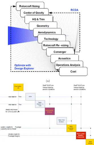
NASA documented a design-from-scratch procedure for rotorcraft design and optimisation1. Fig-ure 1.1(a) is an image from this document showing a simpliﬁed overall design process for heli-copters. Figure 1.1(b) is an expanded version of a part of that process, which involves the design of the rotor. As can be seen, the design of the rotor is an iterative process between various dis-ciplines. However, even within the aerodynamic discipline alone, the process requires a number of iterations that must ﬁt in with constraints that may be due to sizing, material and other such limiting factors, which are not necessarily aerodynamic related. This narrows the aspects of a blade that can be optimised aerodynamically.

NASA also developed a more recent conceptual design tool14 that designs rotorcraft for specific requirements and then analyses the performance for a set of flight conditions and missions. It has the ability to calculate the weight, power and size of typical configurations but allows flexibility in obtaining new concepts. Various components can be added and sized accordingly. The governing equations are simplified methods and most are analytical, although higher order methods such as CAMRAD have been coupled with them19_.

The optimisation for rotor aerodynamics is typically one that is initiated from an already ‘op-timised’ design, to tweak the values of certain design parameters so that more performance is obtained in hover and forward flight. Over time, many studies have been carried out on the effec-tiveness of various design parameters for rotor blades. Leishman’s book13gives some insight in to the significance of each parameter. It also provides some basic theories and effects that the geom-etry of a rotor has on overall performance. In some cases, the significance is large, but the design parameter is optimised for a non-aerodynamic purpose primarily. For example, in the preliminary design of the rotor, the rotor diameter is usually specified according to non-aerodynamic purposes such as storage, gear box ratio, torque limits, stiffness or drooping of stationary blades and so on. However, the rotor diameter does affect the aerodynamic performance of the helicopter, since the bigger the diameter, the better the hover performance because of the lower disc loading and hence the lower the induced velocity and power. In addition, the autorotation capabilities are improved. Another characteristic sometimes affected by non-aerodynamic parameters mentioned is solidity, σ. Aerodynamically, reducing the rotor solidity, reduces the profile power but increases the disc loading and hence induced power. Since there is less lifting area, the angle of attack of the blades may need to be increased to maintain the same lift. Therefore,σ is limited by the stall margin of the blade. In forward flight, a higher solidity is required to maintain the same lift, but the greater theσ, the lower the Figure of Merit (FM).

In his book13, Leishman also gives a basic outline of how to select aerofoils. For hover,

F M =

C_T3/2 √

2

κC_T3/2 √ 2 + σCdo 8 (1.1) = 1

κ+√2.6 σ

( C_L3/2

CD

)₋1 (1.2)

According to Equation 1.2, the aerofoils must have highC_l3/2/Cd.

(26)

high manoeuvre loads, a higher drag divergence Mach number permitting higher ﬂight speeds without too much power loss and noise, a good lift-to-drag over a wide range of Mach numbers to maintain low proﬁle power consumption and low autorotative descent and a low pitching mo-ment to minimise blade torsion momo-ments, vibrations and to keep loads on the control system small.

Usually thickness is kept small to accommodate a higher Mach number. To compensate for the lift, camber is added. In some cases, trailing edge tabs and reﬂex angles are added to highly cambered aerofoils so that high lift and zero moments can be obtained. On the retreating side, where stall is likely to occur, thicker and more cambered aerofoils stall more gently than thin aerofoils with sharp leading edges. To obtain the best performance, a compromise is required.

Martin and Leishman20performed a study on how different tip shapes (rectangular, sweep, taper and subwing tips) in hover affect wake geometry (which is a significant contributor to the per-formance of rotors - especially in hover12 - as it can result in velocity gradients that cause stall on the following blade, high induced velocities and radial flow) and came up with a number of findings. For example, in hover, tip sweep appeared to decrease both radial and axial convection of the core while taper increased radial and decreased axial convection. Also, the primary effect of sweep is that the vortex core is pushed outward past the tip plane path because a swept tip does not conform to the circular streamlines, but is “sheared” so that it extends to outside r/R = 100%. The vortex peak swirl velocity (over tip speed) is a function of vortex strength, core circulation normalised with the farfield value and vortex radius. It is also a function of blade planform (twist, taper and sweep) since these parameters influence the peak bound circulation which influences the vortex strength.

Previously, Caradonna also carried out experiments on wakes and looked speciﬁcally at vortex strength21. His experiments used a hot-wire probe to ﬁnd the wake trajectories and velocities. He used a method similar to that used by Cook22 to separate the velocity induced by the wake and the velocity induced by the rest of the system. Even though there is quite a lot of variabil-ity between vortices, they all seem to have similar appearances to the classic Rankine vortex23. However, as rotor speed increases, the appearance departs from the Rankine vortex. The non-dimensional vortex strength remained, however, independent of tip speed. Furthermore, blade vortices seem to contain all the blade circulation.

Caradonna also wrote a second paper on the use of CFD in rotorcraft design12_{. Some of the} com-promises in the design of the main rotor - such as the tip speed - are pointed out. The compromise here is between transonic flow on the advancing side and stall on the retreating side. However, this is strongly dependent on the aerofoil section, twist, planform and propulsive requirements. For hover, the single most important flow issue is the wake because it is the primary determinant of induced power. For forward flight, it has slightly less significance because the wake is convected away from the blade faster; but its detailed prediction is still required for vibratory loadings, for example.

(27)

was deﬁned as the CT/σ where the blade torsion or pitch link loads increase rapidly (Cm). Also, in general, increasing blade twist increases hub and blade vibratory loads. The paper also provide some suggested solutions such as the use of sweep and taper on the blade tip but also the use of live twist, so that there is azimuthal variation in the twist to obtain a reduction in twist on the advancing side. Some helicopters such as the UH60-A reverse the twist at the tip so that the loss is reduced in forward ﬂight, while maintaining the performance in hover13.

(28)

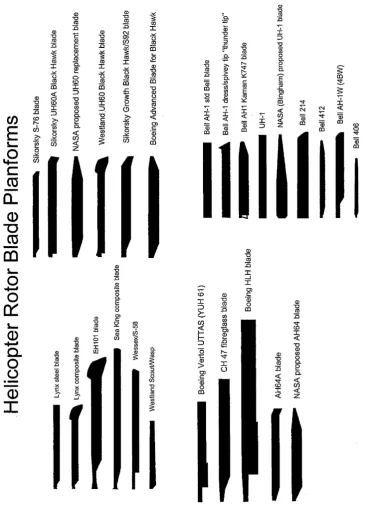
(a)

[image:28.595.139.470.129.635.2]

(b)

(29)

Figure

1.2:

V

arious

blade

planform

[image:29.595.113.487.164.682.2]

(30)

1.3.1 High-ﬁdelity and Low-ﬁdelity Models

Rotor blade optimisation is becoming an increasingly important part of the design process as engineers push the boundaries of rotorcraft efficiency and performance further. However, the development of helicopter rotor optimisation specifically has been slow compared to other rotors such as turbines and compressor blades. This is due to the increased complexity and unsteady nature of the flow around a rotor blade17. Also, the problem is a multi-disciplinary problem involving aerodynamics, aeroelastics, dynamics and flight control coupled to each other. This has lead to the development of comprehensive codes that are able to take into consideration all these disciplines17 by combining modules of codes for each discipline. A recent example of this is the work by Rajmohan et al.25. Here, GT-Hybrid, a CFD solver was coupled with a dynamics code, DYMORE to assess a manoeuvre for a UH60-A rotor. The effects of the blade geometry and wake model fidelity were explored in steady flight comparing loose and tight coupling of the codes. GT-Hybrid was used as a high-fidelity CFD code employing Navier-Stokes equations near the blade and wake models further away. DYMORE uses lifting line theory and an auto-pilot algorithm to perform a fully-trimmed aeroelastic simulation. Differences in the aerodynamics, such as stall on the retreating side, were found to exist even due to the options of loosely and tightly coupling the two codes, suggesting that the coupling of disciplines will be a key part in developing good optimisation tools in the future, when computational power increases and CPU-time is reduced. Biedron and Lee-Rausch26 also used an unstructured flow solver (FUN3D) loosely coupled with with CAMRAD II in comparing experimental and CFD data and how they are integrated for the UH60-A rotor.

Celi also suggests that the optimisation method should be decoupled from the analysis so that it is usable with diﬀerent analysis tools, hence allowing the optimisation technique to use the best version of the analysis code at any time.

Also, the development of optimisation techniques has progressed quite quickly in the structural aspect of rotor design for various objectives such as vibration reduction27, 28. This was not the case on the aerodynamic front due to the lack of modelling techniques17that are both efficient and accurate, although there has been significant improvement. Nevertheless, several authors2, 17, 29, 30 have attempted to devise a variety of successful optimisation techniques. However, each method is typically limited either by the efficiency of the method or the accuracy of the results. The rea-son for this is that high-fidelity CFD simulations are necessary to accurately capture the effects of design changes, especially for rotor aerodynamics but a number of these CFD solutions are required for the process and each calculation can take a long time at a significant computational cost. For example, it was found by Walsh2, who initially optimised a blade without including a wake model for the analysis, that including one had significant contributions to the design of the final optimum rotor blade. Even in the case of fixed-wing aircraft for a single point optimisation problem, the use of higher-fidelity solvers is desirable such as in the work by Rallabhandi and Mavris for sonic boom optimisation31.

To overcome the computational cost problem, a lower fidelity model or metamodel can be used. A metamodel is a model of a model. For this project, it would be a lower fidelity model of the high-fidelity CFD model used to obtain the performance of a number of designs. The metamodel is able to predict the performance of unknown design points a lot faster but with the same ac-curacy as a higher fidelity model. It is able to do this because it is given a reduced number of parameters relative to the CFD method and uses only these parameters to find patterns in the change of the output required. It does this accurately because the data it is provided with, are based on high-fidelity aerodynamic data obtained from CFD.

(31)

of which were selected for validation using the high-ﬁdelity solver and these results were used to update the lower order model.

CFD Methods

In the first attempts at optimisation of rotors, the CFD methods used were simplified. For exam-ple Walsh2 attempted to optimise a rotor in hover while maintaining the performance in forward flight. HOVT (a strip theory momentum analysis with no wake model in the initial analysis) was used to obtain the hover horsepower andCAMRAD, a comprehensive code, for the forward flight horsepower and manoeuvre and trim conditions. Even at this early stage, the idea of using CFD methods for optimisation was attractive. CAMRAD was used because it could be coupled with CFD methods that could be used to obtain better models of effects like transonic effects33. Only some change in the geometry of the blade was captured and hence only a slight improvement was obtained. The conclusions were that further validation and testing would be required.

In the work done by Bohorquez et al.34 _{for optimisation of small rotors where one of the key} objectives was cost-eﬀectiveness, the computational cost of the solutions was further reduced by using incompressible steady calculations with one-equation models of turbulence.

The optimisation by Le Pape and Beaumier35 was coupled with the solver elsA developed by ONERA. Steady RANS was used for the hover calculations. Computations were performed on a coarse grid during optimisation and a fine grid once the minimum was found. In addition, the HOST (Helicopter Overall Simulation Tool) was coupled with elsA, to include aeroelastic and dy-namic disciplines in the analysis (i.e. soft blade), since blade torsion has a significant influence on the aerodynamics of the rotor. So at each optimisation step, the HOST code computed the blade deformation (flap bending and torsion) and the rotor angles (flap and lead-lag) and a new grid was built around the deformed blade and the CFD computed. However, no recomputation of trim was done, making the coupling slightly inaccurate, especially if forward flight was being considered.

Le Pape36 later extended his work to forward flight. elsA was only used for hover optimisa-tion since forward flight calculaoptimisa-tions would take a lot more time and a trimming model would be required as well. HOST was used as the aerodynamic model for the forward flight cases as well as in hover coupled with elsA. It was used as a lifting-line model with a prescribed wake model for forward flight. However, these types of solvers are not very capable of determining the performance of complex blade shapes in forward flight.

Imiela37 optimised the aerodynamic properties of rotor blades considering both hover and for-ward flight using CFD, whilst constraining structural and aeroelastic deformation as calculated by CSD. The solutions were based on high-fidelity CFD/CSM analyses that had weak fluid-structure coupling (i.e. each discipline calculated alternately) combined with an optimisation algorithm. FLOWer was used for the aerodynamic simulation and HOST for blade dynamics and elasticity, although the optimisation itself was focused on aerodynamics. The structural model was not modified during the optimisation.

It can be seen that using a high-fidelity model directly for optimisation of rotor blades is either limited to simpler cases such as hover, or the model’s fidelity is reduced for more complex cases such as forward flying rotors. To be able to model forward flight efficiently, a lower order model is required, but its accuracy still needs to be maintained, especially because of its complexity. Metamodels have this ability.

Metamodels

(32)

data to train the ANN to predict the performance of interpolated design points. The prediction weights were updated using an optimisation algorithm to minimise the error between the network output and the training data (obtained using CFD). The training strategy was enhanced using a GA and gradient-based optimisation. There was no rule for determining the number of nodes in the layer of neurons, but a good initial guess was the average of the input and output nodes. This number was increased to create an optimal-trained network. If the number of nodes was too small, underﬁtting occured, where high error values were obtained and too much generalisation occurred, and vice versa.

In terms of helicopter rotors, optimisation using metamodels has been performed mostly with the aim of vibration and noise reduction such as the work done by Glaz, Friedmann and Liu27, 28. Here, it is suggested that for the particular case of vibration reduction, kriging has proven to be the best surrogate method. However, it brings out the factors that affect the choice of approxima-tion method - such as sampling density, scheme used to select the points and the parameters of the metamodel. It is suggested that since no single metamodel is generically the best, it may be useful to use a combination of metamodels instead. Three metamodels were used viz. polynomial response surface, kriging and radial-basis neural networks. These were combined by a weighted average surrogate algorithm. The conclusions drawn were that the most accurate method de-pended on sample size and the error evaluation method and that the most accurate metamodel did not necessarily produce the best design. Also, in the work done by Liu et al.40, it was shown that for more complicated cases, kriging out-performs RBFs whereas for simpler cases, RBFs are more accurate and efficient. Celi17 also mentioned that the “connection between predictions and accuracy of the optimisation may be more subtle than appears at first glance.”

Imiela37 used DACE41, a MATLAB kriging based metamodel for the optimisation of the rotor in forward ﬂight. Kriging is similar to radial basis function interpolation (RBFs). It is a method of interpolation but the weights involved are driven by the data rather than arbitrary functions. Usually, the weights are functions of the distances of points from the required data point. This means that an estimate of the error is also available. The aim is to determine the weights such that the variance of the estimator is low.42

Kriging is becoming increasingly popular. One reason is because it has few assumptions; in fact the only real assumption is that the design space or equation is continuous43. For example, Glaz et al.44, 45 used it to predict the unsteady lift, drag and moment under dynamic stall for rotor sections on a helicopter blade. The Navier-Stokes equations were used to compute the calcula-tions and the dynamic stall was modelled as a function of time and time history. This non-linear mapping function that is numerically found, linking the input to the output, was modelled using kriging at each time step. In effect, the surrogate model had two dimensions: the kriging for each time step, and the SBRF (surrogate based recurrence framework) to complete the prediction including the time histories. This worked well, with error values falling within 3%. There are a number of types of kriging apart from ordinary kriging, such as universal, co-kriging and blind kriging43. Kriging, however, has been found to be less accurate when the data is sparse43. Marcelet and Peter46 compared the performance of four different metamodels. It was found that kriging and ANN were two of the most accurate methods, and that kriging was more efficient. Ahmed and Qin47 compared RBFs and a number of kriging methods as metamodels to optimise hypersonic spiked blunt bodies. They explain how kriging works and that it can be as good a metamodel if not better than an RBF. Rendall and Allen48 did some work on improving the efficiency of RBFs. Their paper describes a version of RBFs called greedy RBFs whereby the pre-diction of a point is dependent on a smaller selection of points from the entire design space thereby avoiding the calculation of each point’s prediction in relation to the required output. It also lists a number of commonly used basis functions used in RBFs and suggests that the greedy RBF will be useful in compressing data and improving efficiency. This was not verified by other researchers.

(33)

also included a regression model to give it more flexibility in fitting the surface, similar to kriging. In addition, they used t-statistics to determine the significance of each variable to the objective function and hence determine the accuracy of the response surface.

Hajela50 also discusses a number of metamodels used in rotor optimisation such as Immune Net-work modelling, where the design and performance parameters are simulated as antibodies and their corresponding antigens. Their relation is quantiﬁed by a matching function, which works similarly to the ﬁtness value in a Genetic Algorithm (a non-gradient based optimiser).

Other methods include the use of the Fourier transform to predict the flow solver data, as in the work done by Nadarajah and Tatossian51. Their goal was to introduce a Mach number variation into an existing non-linear frequency domain (NLFD) framework and then introduce a time-varying cost function through an adjoint boundary condition to redesign a NASA rectangu-lar supercritical wing. They state that there is a need to develop cost-effective optimal control techniques for unsteady aerodynamics and that an efficient method may be the use of periodic methods such as the Linearised Frequency Domain. However, these methods become highly inac-curate when there are strong non-linearities although further validations with high fidelity software show that this can be overcome52. The efficiency of the NLFD approach is dependent on the pe-riodicity of the flow. In the case of rotor aerodynamics, representing the variations of loading in the frequency domain can lead to a large number of modes required to represent the data as compared to other methods, such as the Proper Orthogonal Decomposition method (POD). The POD method as an interpolation technique was used by Oyama et al.53 to optimise transonic aerofoils for lift/drag ratio. The aerofoils were represented as splines with the design parameters being the control points, and a POD technique was used to obtain the lift-to-drag ratio for new aerofoils that existed on the Pareto front.

A modified version of the POD technique called the Gappy POD method was developed by Will-cox et al.54, 55 for aerodynamic applications. This method is used to interpolate for incomplete or “gappy” data by solving a linear system of equations given a set of POD modes54. Such a method could be used to fill in for incomplete experimental data, or for unknown conditions and even inverse design. In the work done by Gunes et al.,56 a comparison is made of kriging and POD based interpolation to reconstruct the unsteady flowfield around a cylinder. It was found that the POD method is more accurate when there are many snapshots and smaller gaps in the field. When this was not the case, kriging provided a more accurate solution.

Metamodels can be very useful in reducing computational cost and expanding databases as long as they can give accurate predictions that the optimiser can rely on. The usual way of testing the accuracy is to validate an unknown point in the database with its actual value as obtained from the high-fidelity solver. In the work done by Tahara et al.57, where two optimisers were being compared, they introduced an error value which was the difference between the measured and ex-pected improvement by the optimiser. In a similar way, this can be applied to metamodels, where the difference between the predictions and actual values are used to validate the model. If the cost of running an additional set of data is high, another method of testing the prediction accuracy of a metamodel is to use cross-validation43_{. Here, the design space is divided into subsets, and each} one is removed and the metamodel trained without it. It is then reintroduced and compared with its prediction. The average of these is the error. The problem with metamodels is that they fit the existing data but the accuracy of their predictions outside of this trained area is questionable.