PERFORMANCE ANALYSIS OF HARMONIC REDUCTION
BY SHUNT ACTIVE POWER FILTER USING DIFFERENT
CONTROL TECHNIQUES
1R. VENKATESH, 1S.DINESH KUMAR, 2R.SRIRANJANI, 3S.JAYALALITHA
1
PG Scholar, Department of Electrical Engineering, SASTRA UNIVERSITY, Thanjavur 2
Assistant Professor, School of EEE, SASTRA UNIVERSITY, Thanjavur 3
Professor, School of EEE, SASTRA UNIVERSITY, Thanjavur
E-mail:[email protected], [email protected]
ABSTRACT
In modern day power systems the introduction of harmonics due to the presence of non-linear load such as inverters, rectifiers, saturation transformer, electromagnetic interference etc., affects the power quality in distribution systems. This paper is aimed at improving the power quality using shunt active power filter (SAPF). Active filters implemented with the different control techniques under different load conditions are simulated by MATLAB-SIMULINK and their performances are compared.
Keywords: Harmonics, Power Quality, Active Filter, Non-Linear, Matlab-Simulink.
1. INTRODUCTION
Harmonics in power system causes increased line current, neutral current, transformer rating, telephone interference etc. The main cause for the occurrence of harmonics in power system is the usage of linear loads [1]-[2]. These non-linear loads inject harmonics in the power system whose frequency is the integral multiple of fundamental frequency. The harmonics due to non linear load causes increased power loss in power system components such as transformer, transmission line etc., which results in increased heat liberation in the power system components and reduction of self life time of the components. Two types of filters are used for the reduction of harmonics i.e. Active power filter (APF) and passive power filter (PPF) [3]-[4]. PPF uses passive elements such as capacitor, inductor etc...This results in increased power loss, problem of resonance and requirement of separate filter for each harmonic frequency. APF uses active sources such as voltage or current source and power electronic switches to reduce harmonics. APF can be implemented using different techniques. In this paper SAPF is implemented using Instantaneous Reactive Power (IRP) theory and Synchronous Reference Frame (SRF) theory[5]-[8]. The main reason for using APF over passive filter is due to
its wide range of functions such as harmonic elimination, power factor correction, voltage regulation etc. [9]-[10].
2. MODELING OF SAPF
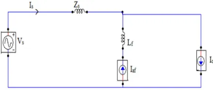
[image:1.595.317.534.552.644.2]The SAPF used in this paper is a voltage source inverter (VSI) which is connected to the load through an interface reactor. Here the harmonic elimination is achieved by injecting harmonic current into the line, which is equal in magnitude and out of phase to load current harmonics.
Figure 1: Generalized Block Diagram of SAPF
2.1 IRP Theory
calculated [2]. The calculated reference current has to be generated by the SAPF and injected to the main line [10].
− − − = c b a e e e e e e 2 / 1 2 / 1 2 / 1 2 / 3 2 / 3 0 2 / 1 2 / 1 1 3 2 0 β α (1) − − − = L c L b L a i i i i i i 2 / 1 2 / 1 2 / 1 2 / 3 2 / 3 0 2 / 1 2 / 1 1 3 2 0 β α (2)
The instantaneous powers at the output side are obtained as follows
− = β α α β β α αβ αβ i i i e e e e e q p
p0 0 0
0 0
0 0
3
2 (3)
0
0 p
p ∗ = − (4)
p
∗αβ=
p
0 (5)0 q
q∗αβ = − (6)
The instantaneous current in α, β, 0
co-ordinates are given by
0 0 * 0 0 _ i e p
ic = = − (7)
∗ ∗ − + = αβ αβ αβ β αβ α α q e e p e e
ic . .
2 2
_ (8)
∗ ∗ + = αβ αβ αβ α αβ β β q e e p e e
ic . .
2 2
_ (9)
Where
e
αβ=
e
α2+
e
β2α _ 0
_ 0.82. . 577 . 0 c c ca i i
i = +
(10)
β
α _
_ 0
_ 0.41 0.707 . 577 . 0 c c c
cb i i i
i = − + (11)
β
α _
_ 0
_ 0.41 0.707
. 577 . 0 c c c
cc i i i
i = − − (12)
Where
i
ca,
i
cb,
i
cc are the compensating [image:2.595.85.518.74.738.2]currents for a, b and c phase
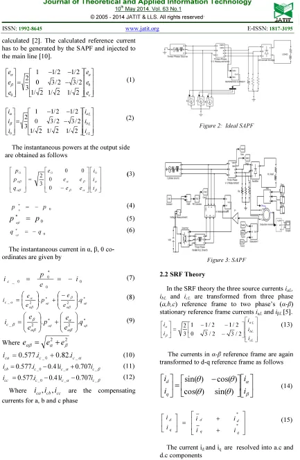
Figure 2: Ideal SAPF
Figure 3: SAPF
2.2 SRF Theory
In the SRF theory the three source currents iaL, ibL and icL are transformed from three phase (a,b,c) reference frame to two phase’s (α-β) stationary reference frame currents iαL and iβL.[5].
− − − = cL bL L a i i i i i 2 / 3 2 / 3 0 2 / 1 2 / 1 1 3 2 β
α
(13)
The currents in α-β reference frame are again transformed to d-q reference frame as follows
−
=
β αθ
θ
θ
θ
i
i
i
i
q d)
sin(
)
cos(
)
cos(
)
sin(
(14) + + = ∗ ∗ q q d d q d i i i i i i (15)The current id and iq are resolved into a.c and
+
−
=
−
− −
q dc d
ref ref
i i i
i
i 1
) sin( ) cos(
) cos( ) sin(
θ θ
θ θ
β
α
(16)
The compensating reference current in a, b, c frame is given by
− − =
− −
− − −
ref ref
ref c
ref b
ref a
i i
i i i
β α
2 3
2 1
2 3
2 1
0 1
3
2 (17)
Figure 4: SAPF Based on SRF Theory
3. SIMULATION RESULTS
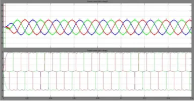
Figure 5: (a) Source Voltage ES (V) (b) Source Current IS (A) (c) Output Current IL (A) for Ideal
[image:3.595.97.516.84.761.2]SAPF with Balanced Load
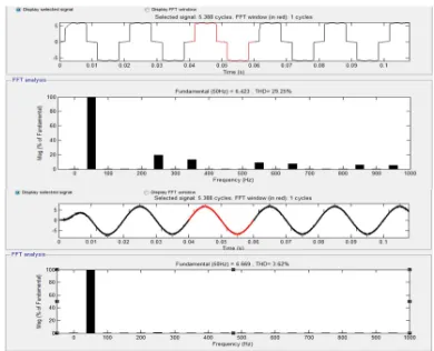
Figure 6: FFT Analysis for Source Current IS (A) in R
Phase of Ideal SAPF with Balanced Load (a) Before Compensation (b) After Compensation
Figure 5 shows the source voltage, source current and load current in case of ideal SAPF and figure 6 shows the FFT analysis of source current for 'R' phase of ideal SAPF before and after harmonic compensation.
Figure 7: (a) Source Current IS (A), (b) Output Current IL (A) for SAPF using IRP Theory with
Balanced Load
Figure 8: (a) Compensating Current IC (A) ,(b)Filter Output Current IF (A) in R Phase of SAPF using IRP
Theory with Balanced Load
Figure 9: FFT Analysis for Source Current IS (A) in R Phase of SAPF using IRP Theory with Balanced
[image:3.595.315.513.219.471.2] [image:3.595.88.282.430.722.2] [image:3.595.315.510.513.671.2]Figure 10: (a) Source Current IS (A) (b) Output Current IL (A) for Shunt Active Filter using IRP
Theory with Unbalanced Load
Figure 11: FFT Analysis for Source Current IS (A) in R Phase of SAPF using IRP Theory with Unbalanced
Load(a) Before Compensation (b) After Compensation
Figure 7 and 10 shows the source current and output current for SAPF using IRF theory with balanced and unbalanced load respectively. Similarly Figure 9 and 11 shows the FFT analysis for ‘R’ phase of source current for SAPF using IRF theory with balanced and unbalanced load. Figure 8 shows the compensating current reference and actual output of the SAPF using IRF theory with balanced load.
Figure 12: (a) Source Current IS (A) (b) Load Current IL (A) for SAPF using SRF Theory with Balanced Load
Figure 13: (a) Compensating Current IC (A), (b) Filter Output Current IF (A) in R Phase of SAPF using SRF
[image:4.595.86.518.72.542.2]Theory with Balanced Load
Figure 14: FFT Analysis for Source Current IS (A) in R phase of SAPF using SRF theory with balanced load(a) Before Compensation (b) After compensation
Figure 12 and 16 shows the source current and output current of SAPF using SRF theory with balanced and unbalanced load. Figure 13 shows the compensating current reference and actual output current of SAPF using SRF theory with balanced load. Figure 14 and 16 shows the FFT analysis of source current before and after harmonic compensation by SAPF using SRF theory with balanced load and unbalanced load.
[image:4.595.315.524.274.428.2] [image:4.595.316.510.589.687.2] [image:4.595.89.282.614.714.2]Figure 16: FFT Analysis for Source Current IL (A) in R Phase of SAPF using SRF Theory with Unbalanced
Load(a) Before Compensation (b) After Compensation
Figure 17: (a) Source Current IS (A), (b) Load Current IL (A) For SAPF using SRF Theory with Dynamic
[image:5.595.82.519.86.732.2]Load (Induction Motor)
Figure 18: FFT Analysis for Source Current IS (A) in R Phase of SAPF Using SRF Theory with Dynamic Load(Induction Motor) (a) Before Compensation
(b) After Compensation
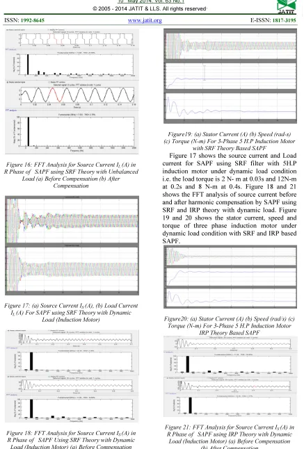
Figure19: (a) Stator Current (A) (b) Speed (rad-s) (c) Torque (N-m) For 3-Phase 5 H.P Induction Motor
with SRF Theory Based SAPF
Figure 17 shows the source current and Load current for SAPF using SRF filter with 5H.P induction motor under dynamic load condition i.e. the load torque is 2 N- m at 0.03s and 12N-m at 0.2s and 8 N-m at 0.4s. Figure 18 and 21 shows the FFT analysis of source current before and after harmonic compensation by SAPF using SRF and IRP theory with dynamic load. Figure 19 and 20 shows the stator current, speed and torque of three phase induction motor under dynamic load condition with SRF and IRP based SAPF.
Figure20: (a) Stator Current (A) (b) Speed (rad/s) (c) Torque (N-m) For 3-Phase 5 H.P Induction Motor
IRP Theory Based SAPF
Figure 21: FFT Analysis for Source Current IS (A) in R Phase of SAPF using IRP Theory with Dynamic
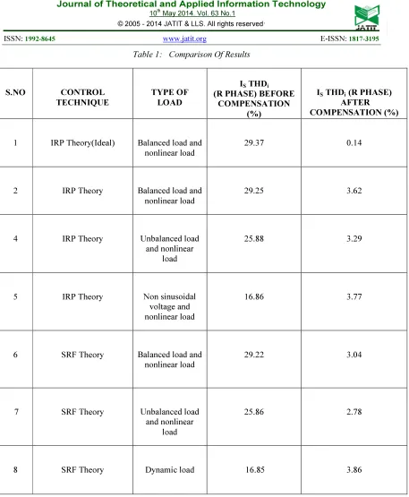
[image:5.595.314.509.436.691.2] [image:5.595.90.281.555.698.2]Table 1: Comparison Of Results
S.NO CONTROL
TECHNIQUE
TYPE OF LOAD
IS THDi
(R PHASE) BEFORE COMPENSATION
(%)
IS THDi (R PHASE)
AFTER COMPENSATION (%)
1 IRP Theory(Ideal) Balanced load and
nonlinear load
29.37 0.14
2 IRP Theory Balanced load and
nonlinear load
29.25 3.62
4 IRP Theory Unbalanced load
and nonlinear load
25.88 3.29
5 IRP Theory Non sinusoidal
voltage and nonlinear load
16.86 3.77
6 SRF Theory Balanced load and
nonlinear load
29.22 3.04
7 SRF Theory Unbalanced load
and nonlinear load
25.86 2.78
8 SRF Theory Dynamic load 16.85 3.86
From the comparison table it is found that for ideal SAPF using IRP theory, the source current Total harmonic distortion (THDi)
reduced from 29.37% to 0.14% .Incase of SAPF using IRP theory the THDi reduced from
29.25% to 3.62% for balanced load and 25.88% to 3.29% for unbalanced load. For SAPF using SRF theory with balanced load the source current THDi reduced from 29.22% to 3.04%.(All THDi
are measured for R phase).For Dynamic load condition the source current THDi reduced from
16.86% to 3.77% in SAPF using IRP theory and the source current THDi reduced from 16.85% to
5. CONCLUSION
Modeling of SAPF using IRP theory and
SRF theory is done using
MATLAB-SIMULINK and THDi of source current is
analysed for before and after compensation for various load condition and obtained conclusions are summarized as follows (1) source current THDi is reduced to a considerable amount of
around 3% which is within the limits of IEEE 519 standards.(2)Both IRP and SRF theories are found to be efficient in eliminating harmonics in case of dynamic load.
REFERENCES:
[1].Udom,Khruathep,SuittichaiPremrudeepreec hacharn,YuttanaKumsuwan,
[2].“Implementation of shunt active power filter using source voltage and source current detection”, IEEE, ,2008, pp. 2364-2351. [3].H. Akagi, Y. Kanazawa, A. Nabae,
“Instantaneous reactive power
compensator’s comprising switching device without energy storage components,” IEEE Trans. Ind. Applications,vol. .IA-20, May/June 1984. pp. 625-630
[4].Reyes H. Herrera, Patricio Salemeron, Hoyosung Kim,“Instantaneous Reactive Power Theory Applied to Active Power Filter Compensation: Different approaches, Assessment, and Experimental Results”,
IEEE, Trans. On Industrial Electronics, pp. 184-196, 2008.
[5].Chandra A, Singh B, Al-Haddad K, “An improved control algorithm of shunt active filter for voltage regulation, harmonic elimination, power factor correction, and balancing nonlinear loads”, IEEE Trans. on Power Electr, pp. 495-503,2000.
[6].R..Sriranjani and S.Jayalalitha, “
Improvement of the time domain
specifications of DC bus voltage of shunt active filter using controllers”, IEEE International Conference on recent advancement in Electrical, Electronics and Control Engineering, Mepco Schlenk Engineering College, pp(187-191),2011. [7].Chennai Salim , Benchouia M-T,
“Three-Phase Three-wire Shunt Active Power Filter Based on Hysteresis, Fuzzy and MLPNN Controllers to Compensate Current Harmonics” Journal of Electrical and Control Engineering Vol. 3 No. 3, 2013
[8].R.Sriranjani and S.Jayalalitha, “Investigation the performance of various types of filter”,WASJ, Vol 17, no.5, pp 643-650, 2012.
[9].R.Sriranjani , M.Geetha and S.Jayalalitha,
“Harmonics and reactive power
compensation using Shunt Hybrid
filter”,RJASET ,5(1), 2013.
[10]. Vijayakumar.A, .Mahendra Babu. T.K, “A novel approach for mitigation of harmonics and interharmonics in variable frequency drives”,JATIT, 59,2,pp. 360 – 366 , 2014