Variational models and numerical algorithms for effective image registration

(1)

Variational Models and Numerical Algorithms for Effective Image

Registration

by

Mazlinda Ibrahim

under the supervision of

Professor Ke Chen

Thesis submitted in accordance with the requirements of the University of Liverpool for the

degree of Doctor in Philosophy.

(2)

Acknowledgment

I would like to express my gratitude to my supervisor Prof. Ke Chen for his guidance and patience throughout my studies. Not to forget my second supervisor Dr. Bakhti Vasiev for his support and encouragement. I also would like to thank Prof. Alexander Movchan as the head of Department of Mathematical Sciences as well as Dr. Martyn Hughes for their advice during my doctoral studies.

In this very special moment, I would like to thank all the CMIT’s members including Dr. Bryan Williams, Dr. Jianping Zhang, Dr. Lavdie Rada, Dr. Carlos Brito-Loeza and Jack Spencer for all the valuable time, advice, criticism and discussion. Indeed, this entire journey helped me to obtain better understanding of many valuable things in this life.

A gigantic thank you to my family: Ma, Abe Kie, Akak, Lina, Juwe, Udin, Kak Izan, Abang Yahaya, Abang Yie, Aqilah, Alia and Adwa. This thesis is dedicated to my late father Ibrahim Ismail, who passed away five months before I started my doctoral studies. In addition, my sincere appreciation to Dr. Bryan Williams, as my friend and unpaid English tutor. Not to forget Dr. Juriah Kamaludeen, Dr. Alia Ruzanna Aziz, Noor Hakim Ahmad, Aznida and Esraa Tarawneh for their support and encouragement. We had a great time in Liverpool for almost four years with exciting activities. I also would like to thank Hoo Yann Seong who is always next to me and ready to lend her ears. Thank you so much, Hoo!

(7)

Abstract

The goal of image registration is to align two or more images of the same scene obtained at different times, from different perspectives, or sensors such as MRI, X-ray and CT. This step is required to facilitate automatic segmentation for tumour detection or to inform further decisions in treatment planning. It is an important and challenging sub-ject which usually involves high storage, computational cost and dealing with distorted and occluded data. The paradigm behind image registration is to find a reasonable transformation so that the template image becomes similar to the so-called given ref-erence image. Through such transformation, information from these images can be compared or combined. This thesis deals with the mathematical modelling of image registration by way of energy minimisation of a functional.

We propose a new decomposition model for image registration which combines para-metric transformation and non-parapara-metric deformation. The first category of methods is based on a small number of parameters and for the second category the transforma-tion is based on a functransforma-tional map (or discretely a large number of parameters) with a regularisation term. We choose one cubic B-spline based model and the linear curva-ture model for the parametric and non-parametric parts respectively where the overall deformation consists of both global and local displacement for effective image regis-tration. Some results for synthetic and real images will be presented to illustrate the effectiveness of the new model in contrast with the individual models.

We then propose a novel variational model for image registration which employs Gaussian curvature as a regulariser. The model is motivated by the surface restoration work in geometric processing [21]. An effective numerical solver is provided for the model using an augmented Lagrangian method. Numerical experiments show that the new model outperforms three competing models based on, respectively, the linear curvature [24], the mean curvature [19] and the diffeomorphic demon models [93] in terms of robustness and accuracy.

(8)

List of Figures

1.1 Illustration of reference and template images for multi-modality image registration. The same objects in the reference (a) and template images (b) have different intensity values. . . 2 1.2 Illustration of reference and template images. The template image (b)

is a rotated version of the reference image (a). . . 3

2.1 From left to right: the graphs of the functionsf(x),g(x) andh(x) where

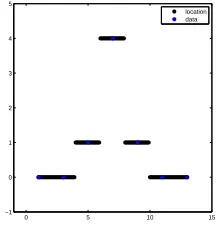
f(x) andg(x) are of bounded variation for Ω = [0,1]. The functionh(x) has infinite total variation and is the space nor a bounded variation function. . . 14 2.2 On the left is the given grey level imageu(x) and on the right some of

its λ-level curves, these are curves whereu(x) =λfor someλ= [0,1]. . 16 2.3 Illustration of (a) cell-centred discretisation and (b) vertex-centred

dis-cretisation on a square mesh. Red crosses show the cell-centred points and the red boxes show the vertex grid points. . . 20 2.4 Illustration of the ghost points outside the domain using vertex-centred

discretisation. The grid points are represented by the blue circles and the white circles are the ghost points. . . 22 2.5 Illustration of a pyramid of grid with four levels. Red crosses are the

cell-centred discretisation points. . . 32 2.6 Illustration of the standard coarsening strategy. The fine grid in (a)

has 9×9 discretisation points. An example of semi-coarsening where the coarse grid in (b) is obtained by doubling the mesh size in the x1 -direction. In (c), we obtained the coarse grid by doubling the mesh size in thex2-direction. Finally, the coarse grid (d) is constructed using these

standard procedures. . . 34 2.7 Illustration of the restriction operators. (a) is the injection operator, (b)

(9)

2.8 Illustration of bilinear operator from the coarse grid to the fine grid. The coarse point in black circles are used to obtain the nine fine points surrounding it. . . 35 2.9 Illustration of multigrid cycles with three levels of grid. Left is the

V-cycle and on the right is the W-V-cycle. The white circles denote the coarsest grid, \ and / denote the restriction and interpolation steps, respectively. . . 36

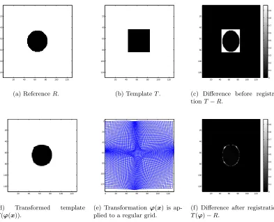
3.1 Illustration of an image registration problem. Reference and template images are given in (a) and (b) respectively. The difference before regis-tration is given in (c) and (d) is the transformed template image using the transformation in (e). (f) is the difference image after registration and we can observe that the difference image is reduced after registra-tion. Notice that the transformed template image looks similar to the reference image after registration. . . 42 3.2 Illustration of translation, rotation, scaling, shearing and projective

trans-formation for the image I. . . 45 3.3 Illustration of nearest neighbour interpolation in a 1D problem. . . 54 3.4 Illustration of linear interpolation in a 1D problem. . . 55 3.5 Illustration of Runge phenomenon using higher order polynomial

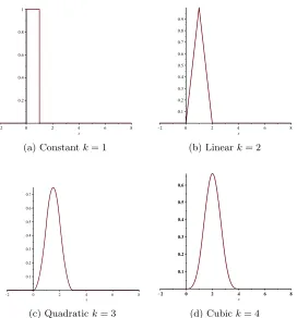
inter-polation. . . 55 3.6 Illustration of basis functions for k= 1,2,3,4. . . 57 3.7 Illustration of an image segmentation problem. (a) is the image to be

segmented because the image appears dark and the boundaries of the objects are not clearly visible. (b) shows the binary representation of the image in (a) where white pixels represent the edges of the object in (a). . . 59

4.1 Plots of three energy terms to aid choice ofγp and γnp. . . 75 4.2 Top row and left to right: template, reference and the difference between

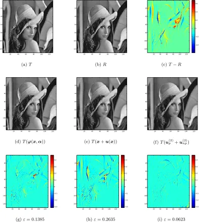
the template and reference images. Middle row and left to right: results of Test 1 using M1, M2, and M3. Bottom row shows the differences of the transform template images (middle row) and reference images. All three models are able to register Test 1 but a smaller value ofεis given by M3. . . 77 4.3 First to second row and left to right: deformation field applied to the

(10)

4.4 Top row and left to right: template, reference and the difference between the template and reference images. Middle row and left to right are the results of Test 2 using M1, M2, and M3. Bottom row shows the differences of the transform template images (middle row) and reference image. The best result is given by M3 where we can see that the method gives the smallest error as depicted on the bottom row. . . 80 4.5 First to second row and left to right: deformation field applied to the

regular grid for Test 2 using M1,M2,M3 after the parametric part and M3 after the non-parametric part. Third to fourth row and left to right: the values of the determinant of the Jacobian matrix for the correspond-ing deformation on the top row. It is clear that the determinant of the Jacobian matrix is positive everywhere. . . 83 4.6 First to second row and left to right: template, reference and the

differ-ence between the template and referdiffer-ence images. Middle row and left to right, are the results of Test 3 using M1, M2 and M3. Bottom row is the differences of the transform template images (middle row) and reference image. The best result is given by M3 where we can see that the method gives the smallest error as depicted on the bottom row. . . 84 4.7 Top row and left to right: deformation field applied to the regular grid

for Test 3 using M1,M2,M3 after the parametric part and M3 after the non-parametric part. Bottom row and left to right: the values of the determinant of the Jacobian matrix for the corresponding deformation on the top row. It is clear that the determinant of the Jacobian matrix is positive everywhere. . . 85 4.8 Top row and left to right: template, reference and the difference between

the template and reference images. Middle row and left to right: trans-formed template using M1, M2 and M3. Bottom row: the respective differences between the transformed template with the reference images. The corners of the boxes are well captured with M3 compared to M1. . 86 4.9 First to second row and left to right: deformation field applied to the

regular grid for Test 4 using M1,M2,M3 after the parametric part and M3 after the non-parametric part. Third to fourth row and left to right: the values of the determinant of the Jacobian matrix for the correspond-ing deformation on the top row. It is clear that the determinant of the Jacobian matrix is positive everywhere. . . 87

5.1 Illustration of the image R and the joint probability density for R. (a) is the imageR, (b) shows that the density is very ‘sharp’ becauseR=R

(11)

5.3 Comparison of two distance measures. (a) is the reference image R, (b) is mutual information and (c) is normalised gradient field as the distance measures. We can see that (b) is highly convex. Thus, non-convexity of registration problems increases with mutual information as the distance measure. . . 98 5.4 Test 1: Results of mutual information as the distance measure with

the decomposition model for multi-modality images. We can see that the model delivers a good alignment between the transformed template image in (d) and the reference image in (b). . . 104 5.5 Test 1: Results of normalised gradient as the distance measure with the

decomposition model for multi-modality images. The resulting trans-formed template in (b) is in alignment with the reference image except at the middle part of the brain. Smaller value of DMI₍_T₍_ϕ₍_x₎₎_{, R}_{) in}

(b) than in Figure 5.4 (d) indicating higher similarity between the trans-formed template and the reference images. . . 105 5.6 Test 2: Results of mutual information as the distance measure with the

decomposition model for multi-modality images. We can see that the model fails for the deformed circle in the template image in (a) due to the existence of the inner square in the reference image (b). . . 106 5.7 Test 2: Results of normalised gradient as the distance measure with the

decomposition model for multi-modality images. We can see the model is able to solve this particular problem. Smaller value ofDMI₍_T₍_ϕ₍_x₎₎_{, R}₎

in (b) than in Figure 5.6 (d) indicating higher similarity between the transformed template and the reference images. . . 106 5.8 Test 3: Results of mutual information as the distance measure with the

decomposition model for multi-modality images. We can see that the model fails to register the template with the reference image due to the strong bias field in (a). . . 107 5.9 Test 3: Results of normalised gradient field as the distance measure with

the decomposition model for multi-modality images. We can see that the model fails to register the template with the reference image due to the strong bias field in (a). Smaller value of DMI₍_T₍_ϕ₍_x₎₎_{, R}_{) in (b) than}

in Figure 5.8 (d) indicating higher similarity between the transformed template and the reference images. . . 107

(12)

6.2 Location of a surface’s saddle point by GC and MC. (a) is the surface with a saddle point. (b) is the negative mean curvature and (c) is the negative Gaussian curvature. The highest point in (b) is not at the saddle point and for (c), the saddle point is better distinguished from its neighbourhood. . . 115 6.3 Test 1 (X-ray of hand). Illustration of the effectiveness of Gaussian

cur-vature with smooth problems. On the top row, from left to right: (a) template, (b) reference and (c) the difference before registration. On the bottom row, from left to right: (d) the transformation applied to a regular grid, (e) the transformed template image and (f) the difference after registration. As can be seen from the result (e) and the small dif-ference after registration (f), Gaussian curvature is able to solve smooth problems. . . 122 6.4 Test 1 (X-ray of hand). Comparison of Gaussian curvature with

com-peting methods. The transformed template image using (a) Model D, (b) Model LC, (c) Model MC and (d) Gaussian curvature. Note the difference of these three images inside the red boxes. . . 123 6.5 Test 1 (X-ray of hand). Comparison of transformed templates in

zoomed-in boxes and their localεvalues: (a) Model D, (b) Model LC, (c) Model MC and (d) Gaussian curvature. Gaussian curvature has the smallestε

value. . . 124 6.6 Test 2: A pair of Brain MR images. Illustration of the effectiveness of

Gaussian curvature with real medical images. On the top row, from left to right: (a) template, (b) reference and (c) the difference before regis-tration. On the bottom row, from left to right: (d) the transformation applied to a regular grid, (e) the transformed template image and (f) the difference after registration. As can be seen from the result (e) and the small difference after registration (f), Gaussian curvature can be applied to real medical images and is able to obtain good results. . . 125 6.7 Test 2: A pair of Brain MR images. Comparison of Gaussian curvature

with competing methods. The transformed template image using (a) Model D, (b) Model LC, (c) Model MC, and (d) Gaussian curvature. Notice the differences of these three images inside the red boxes. Con-siderably more accurate results are obtained, particularly within these significant regions, by employment of the Gaussian curvature model. . . 126 6.8 Test 2: A pair of Brain MR images. Comparison of transformed

(13)

6.9 The effects on the values of F and ε for various values of γ are shown in (a) and (b). We obtain these figures using r = 0.02 for Test 1 and it confirms that γ controls the smoothness of the deformation field. The iteration history for Test 1 is shown in (c). Since the functional J is decreasing, the convergence of the proposed model is confirmed. . . 127 6.10 The effects on the value of F, n1, n2 and ε for various values of r. In

(a), F decreases with decreasing value of r. We should use the value of r, such that F > 0, to avoid mesh folding. In (b), we can see that increasing the value ofr will decrease the difference betweenq1,q2 and ∇u1,∇u2. From (c), with a large value of r, we have smaller residual indicated by n2. In (d), although smallr = 0.002, gives a very smallε, but since F <0 for this value of r, we choose the optimal value of r to ber = 0.02. . . 128 6.11 Results of Gaussian curvature image registration for multi-modality

im-ages. The model is able to register multi-modality images with mutual information as the distance measure. . . 129

7.1 Test 1: GV-JSR model. Illustration of the type of images where the GV-JSR model delivers good results where the object to be segmented in the template image is relatively large. The results obtained in this test are forα=β= 25. . . 140 7.2 Test 2: GV-JSR model. Illustration of the second class of problems

where the GV-JSR model manages to provide good results where the deformation of the features inside the object to be segmented pose the same deformation as the object itself. . . 141 7.3 Test 3: GV-JSR model. Illustration of the type of image which has

different deformation for the boundary Γ and the features inside Γ. The GV-JSR model fails to align the features inside Γ but manages to align the outer most square in the template image. In this test we are using

α= 5 and β= 25. . . 142 7.4 Test 3: NJSR model. We have better results using the NJSR model for

Test 3 where the circles in T are deformed to squares as in R. We also have smaller value of ε= 0.0062 for the NJSR model than ε= 0.0509 which is obtained from the GV-JSR model. . . 143 7.5 Test 4: GV-JSR model. The model fails when there is more than one

(14)

(15)

List of Tables

4.1 Comparison of MSE, and the dice metric for white and grey matter for segmented images of Test 3 before registration, and after registration using M1, M2 and M3. Clearly M3 is the best. . . 79 4.2 Comparison of MSE, and the dice metric for white and grey matter for

segmented images of Test 3 for N = N1 = N2 = 129 before registra-tion, and after registration using M1, M2 and M3. Our method M3 outperforms M1 and M2. . . 81 4.3 MSE, and the dice metric for Test 4 before registration, and after

regis-tration using M1, M2 and M3. MSE is decreasing for all three models with the lowest value given by M3. The dice metrics are increasing for all models where the highest value is given by M3. Our method M3 outperforms the individual methods. . . 81

6.1 Quantitative measurements for all models for Test 1. ML and SL stand for multi and single level respectively. γ is chosen as small as possible such that F > 0 for all methods. F > 0 indicates the deformation consists of no folding and cracking of the deformed grid. We can see that the smallest value ofε is given by Gaussian curvature (GC). . . . 123 6.2 Quantitative measurements for all models for Test 2. ML and SL stand

(16)

Publications

A Decomposition Model and Its Algorithm Combining Cubic B-spline and Non-parametric Deformation for Effective Image Registration. Mazlinda Ibrahim and Ke Chen. In preparation.

A Unifying Framework for Decomposition Models of Parametric and Non-parametric Image Registration. Mazlinda Ibrahim and Ke Chen. Submitted to Neurocomputing.

A Novel Variational Model for Image Registration using Gaussian Curva-ture. Mazlinda Ibrahim, Ke Chen and Carlos Brito-Loeza. Journal of Geometry, Imaging and Computing. 1(4):417-446, 2014.

An Improved Model for Joint Segmentation and Registration. Mazlinda Ibrahim, Ke Chen and Lavdie Rada. In preparation.

Presentations

A Decomposition Model Combining Parametric and Non-parametric Defor-mation Image Registration.

22th International Symposium on Mathematical Programming, 12-17 July 2015, Pitts-burgh.

A Composition Model Combining Parametric Transformation and Non-parametric Deformation for Effective Image Registration.

SIAM Conference on Imaging Science, 12-14 May 2014, Hong Kong. Fourth Order Variational Formulation for Image Registration. 25th Biennial Conference in Numerical Analysis, 25-28 June 2013. Glasgow.

An Improved Model for Joint Segmentation and Registration based on Lin-ear Curvature Smoother .

3rd International Workshop on Image Processing Techniques and Applications, incor-porating Mathematical Imaging with Biomedical Application, 6-8 July 2015. Liverpool. A New Variational Model for Image Registration using Gaussian Curvature. LMS Inverse Day on Tomographic Reconstruction from Boundary Data, 22 September 2014. Leeds.

Improved Parametric and Non-parametric Image Registration.

(17)

Chapter 1

Introduction

Image registration, also known as warping, fusion, motion correction or co-registration is one of the most difficult tasks among medical imaging applications. Another chal-lenging task is image segmentation. Registration aims to automatically align images and establish correspondences between features within images which display different views of the same objects. Such images may be taken from different individuals, at different times or from different imaging machineries. After successful registration, in-formation from different images may be compared, combined or fused for further tasks. There exits a large number of application areas for image registration including compu-tational anatomy [1], computer aided diagnosis [92], radiation therapy [100], treatment verification [27], CCTV [76] and remote sensing [61].

For example, in medical imaging, a radiologist may be asked to combine information from computer tomography (CT) and photon emission tomography (PET) where the former modality contains patient anatomy information such as bones and organs while the latter modality is used to scan the functional data such as glucose uptake. The CT imaging process requires the patient to rest his arms due to space limitation in the CT tube. For PET scanning, the patient needs to lift his arm to minimise attenuation of the tracer. Image registration aims to align these two data of data into a unified spatial alignment. The job becomes harder since there is no motion model for each patient and internal organs move according to individuals. In [8], the authors mention that quantification and evaluation of registration results are difficult because there is not much information about the ground truth for the registration of medical images.

(18)

1.1 Introduction to Image Registration

Image registration is the process of finding geometric transformation between two given images respectively known as the template (target) and reference (source) images. The recovered transformation may be applied to the template image so that it becomes similar in some sense to the reference image. It is assumed that the template image is a deformed version of the reference image. Image registration has broad applications ranging from medical image analysis, video surveillance, remote sensing and satellite imagery. For mono-modality image registration, images are generated from the same imaging machinery. Thus, the same objects or features in the images are represented by the same intensity values. In this case, finding the optimal transform which links the two images remains a challenging subject. Meanwhile, for multi-modality image registration, images are generated from different imaging machineries. Thus, the same objects or patterns will have different intensity values as shown in Figure 1.1. Conse-quently, matching patterns is a challenge.

20 40 60 80 100 120 20

40

60

80

100

120

(a) Reference image,R.

20 40 60 80 100 120 20

40

60

80

100

120

(b) Template image,T.

Figure 1.1: Illustration of reference and template images for multi-modality image registration. The same objects in the reference (a) and template images (b) have different intensity values.

(19)

Since the goal of image registration is to transform images such that they become similar, modelling the problem involves the minimisation of a dissimilarity functional. The functional can either be a function of the image intensity difference or a distance between landmarks or markers in the images. In the former case, the registration process is given implicitly by the whole image and in the latter case, only some parts of the image are used to identify the deformation field.

In order to illustrate mono-modality image registration, we refer to Figure 1.2 where

20 40 60 80 100 120 20

40

60

80

100

120

(a) Reference image,R.

20 40 60 80 100 120 20

40

60

80

100

120

(b) Template image,T.

Figure 1.2: Illustration of reference and template images. The template image (b) is a rotated version of the reference image (a).

the reference image (a) consists of a rectangle and, in the template image (b), this rectangle is rotated. In image registration, we are looking for the transformation which may be applied to the rectangle in T, in order to transfigure it to be similar to the reference imageR. We can use the following dissimilarity or similarity measure which is the sum of the squared difference (SSD),

DSSD(T, R,ϕ(x1, x2)) =

1 2

Z

Ω

(T(ϕ(x1, x2))−R(x1, x2))2dΩ (1.1)

whereϕis the transformation, dΩ = dx1dx2and Ω is the image domain. The distance in equation (1.1) is the L2 norm and it should be noted that minimising (1.1) with

respect to the transformation ϕ is an ill-posed problem. This is because the solution given by

min

ϕ D

SSD₍_{T, R,}_ϕ₎ _(1.2)

is not unique. Referring to Figure 1.2, the solution can be either a rotation of π₂ or

−3₂π about the centre of the image. Thus, we need a priori information about the transformation so that unwanted solutions may be penalised. Using the well-known Tikhonov regularisation, we incorporate a regularisation term S(ϕ) into (1.1). The joint energy minimisation functional corresponding to (1.1) consists of a weighted sum including fitting and regularisation terms as follows,

(20)

where γ is a positive constant parameter which balances the trade-off between the fitting and regularisation energies. This thesis focuses on mathematical models of image registration based on this type of variational approach.

1.2 Thesis Outline

The remaining chapters of this thesis are organised as follows.

Chapter 2 - Mathematical Preliminaries

In this chapter, we present some mathematical tools which will be used throughout this thesis and which the reader may wish to consult while reading subsequent chapters. A brief review is given of definitions, theorems and examples of some important and relevant mathematical topics including normed linear spaces, variations of a functional, functions of bounded variation, inverse problems and regularisation, the discretisation of partial differential equations using finite differences, and iterative solutions of linear and nonlinear equations. Finally, we will conclude this chapter with an introduction to the multigrid method for elliptic PDEs.

Chapter 3 - Mathematical Models for Image Registration and Segmentation

In this chapter, we present a brief review of mathematical models for image registration. We start with the mathematical setting for an image and the mathematical formula-tion for image registraformula-tion. We introduce similarity measures and parametric image registration models. Then, we cover some existing models for non-parametric image registration based on the variational formulation such as the linear elastic, nonlinear elastic and fluid registration techniques. We also introduce and describe a solution scheme for the minimisation of such models. We finally present some work in image segmentation which is useful for Chapter 7.

Chapter 4 - A Decomposition Model Combining Parametric and Non-parametric Deformation

In this chapter, we introduce a decomposition model for mono-modality image registra-tion which combines parametric transformaregistra-tion and non-parametric deformaregistra-tion. We choose cubic B-spline and linear curvature to model parametric and non-parametric transformations respectively. Numerical results are presented at the end which show that the decomposition model outperforms individual models.

Chapter 5 - Multi-modality Image Registration using the Decomposition Model

(21)

reference and template images come from different imaging modalities. For example, the reference image may be a computer tomography (CT) scan which is good for the quantification of cancerous tissues for determining the dose calculation in treatment planning and the template image may be a magnetic resonance (MRI) image which is much better for the visualisation of soft tissues compared to the CT scanner. Given the very different resulting images, the intensity values are not directly comparable and so the use of traditional similarity measures such as the sum of the squared difference is no longer valid. We explore two similarity measures for multi-modality images given by mutual information and the normalised gradient field in order to build registration models for such images. We use three data sets in order to test these two similarity measures with the decomposition model.

Chapter 6 - A Novel Variational Model for Image Registration using Gaus-sian Curvature

In this chapter, we propose a novel regularisation term for non-parametric image regis-tration based on the Gaussian curvature of the surface obtained from the displacement field. Direct solution of the resulting Euler-Lagrange PDEs is difficult due to high nonlinearity. We provide a numerical solver for the model using the augmented La-grangian method. Numerical experiments are shown to illustrate the performance of the proposed model in comparison with the linear curvature, diffeomorphic demon and mean curvature models. Our new model turns out to be more robust than these three competing models for the tested images because Gaussian curvature is a more natural physical quantity for a surface compared to linear and mean curvatures.

Chapter 7 - An Improved Model for Joint Segmentation and Registration

In this chapter, we present an improved model for joint segmentation and registra-tion using the active contour without edges method for segmentaregistra-tion and the linear curvature model for image registration. The proposed model improves on the original Guyader and Vese model [58] for image segmentation and registration. Here we use the Chan-Vese model for segmentation [12] where the image is modelled as a piecewise constant function.

Chapter 8 - Conclusion and Future Research

(22)

Chapter 2

Mathematical Preliminaries

This chapter covers some basic mathematical tools that will be used throughout the thesis. We begin with an introduction to normed linear spaces with some useful ex-amples. Next, we review some relevant theory about calculus of variation. We discuss inverse problems and regularisation before moving on to the discretisation of partial differential equations (PDEs) by finite difference methods and define some notation. Finally, we discuss iterative methods and iterative solutions of nonlinear equations, finishing with an introduction to multigrid methods.

2.1 Normed Linear Spaces

Definition 2.1.1 Linear Vector Space. Let V be a set with the operations of mul-tiplication and addition defined. Letu and v be any two elements of V, u,v∈V. Let the sum of these two elements be denoted by u+v and the scalar multiplication of u

with an element c ∈F of a scalar field F by cu. Then V is called a vector space of a scalar field F if all of the following ten axioms are satisfied.

1. Closure under addition: u+v∈V.

2. Commutativity under addition: u+v=v+u.

3. Associativity under addition: (u+v) +w=u+ (v+w) for all w∈V.

4. Existence of an identity element of addition: There exists an element0∈V, such that0+u=u for all u∈V.

5. Existence of additive inverse: For all u ∈ V, there exists an element −u ∈ V, such thatu+−u=0.

6. Closure under scalar multiplication: For c∈F, we have cu∈V. 7. Distributivity: If u,v∈V and c∈F, then c(u+v) =cu+cv.

8. Distributivity under scalar multiplication: Ifc, d∈F, then (c+d)u=cu+du. 9. Associativity under scalar multiplication: If c, d∈F, then c(du) = (cd)u.

10. Existence of an identity element of scalar multiplication: There exists an element

(23)

Example 2.1.2 The linear vector spaces denoted by

• _Rd _and

Cd for all d∈N,

• F[x], a polynomial function over a fieldF,

are normed linear spaces. We can verify these using Definition 2.1.

Theorem 2.1.3 Linear Subspace. A subset W of a vector space V is a linear sub-space if and only if it satisfies the following three properties:

1. There exists 0∈W.

2. W is closed under addition.

3. W is closed under scalar multiplication.

Proof The first property ensures that W is not a null set since there exists at least one element of W. From the definition of vector space and since an element of W is also an element of V, the vector space operations are well defined.

Definition 2.1.4 Norm and Seminorm. A norm k · k on a vector space V is a functionk · k:V→_R that satisfies the following properties for allu,v∈V and λ∈F

where F is a scalar field.

1. Faithfulness: kuk= 0 if and only if u= 0 and kuk>0 if u6= 0. 2. Homogeneity: kλuk=|λ|kuk.

3. Subadditivity: ku+vk ≤ kuk+kvk.

A semi-norm is defined similarly as above but with the first property being replace by

kuk ≥ 0. A normed space is a linear vector space with a norm defined on it. For a normed linear space, the distance (also known as a metric) between two elements

u,v∈V is denoted by d(u,v) =ku−vk.

Example 2.1.5 p-norm. Let x ∈Rn, then for any real number p ≥1 we define the

p-norm of x as

kxk_p= n X

i=1 |x_i|p

!1_p

.

Forp= 2, we recover the Euclidean norm defined by

kxk_Rd =

√

x·x= v u u t

n X i=1

x2_i.

The Euclidean scalar product is denoted by x·y and is defined by

x·y=kxkkykcosθ

(24)

Example 2.1.6 Lp-norm or Lp-norm . Letf be a function defined on a domainΩ

and 1≤p≤ ∞. We define the Lp_{-norm of} _f _on_Ω _as

kf(x)k_p = Z

Ω

|f(x)|pdx

1_p

.

Note that since f may have arbitrarily many components, this is a generalisation of Example 2.1.5.

Example 2.1.7 L∞-norm. The special case of the Lp-norm from Example 2.1.5 where p=∞ is defined as

kf(x)k∞= sup

x

|f(x)|. (2.1)

Definition 2.1.8 Inner Product. An inner product on a linear vector space V de-fined over the scalar field F is a function h·,·i_V defined on V×V which satisfies the following properties:

1. Positive definiteness: hu,ui_V >0 for u6=0 and u∈V. 2. Conjugate symmetry: hu,viV=hv,ui_V for all u,v∈V.

3. Linearity under scalar multiplication: hλu,viV =λhu,viV for all u,v ∈V and

λ∈F.

4. Linearity under vector addition: hu+v,wiV =hu,viV+hv,wiV for allu,v,w∈

V.

Example 2.1.9 Examples of inner products are

• The standard inner product

hx,yi_Rd =y>x=

d X i=1

xiyi

for allx,y∈_Rd_.

• If C[a, b] is the vector space of real-valued continuous functions defined on the interval (a, b), then

hf, gi= Z b

a

f(t)g(t) dt

is an inner product on C[a, b].

Definition 2.1.10 Support of a Function. Let Ω be a nonempty open set in Rn,

and let f be a continuous real or complex valued function on Ω. The support of f is defined as

supp(f) ={x∈Ω :f(x)6= 0}. (2.2)

Definition 2.1.11 Compactly Support. A function f in Ω⊂_Rn _{has compact}

(25)

Definition 2.1.12 Cauchy Sequence and Completeness. A sequence{xi}i∈Nin a

normed vector spaceV is called a Cauchy sequence if for any real number, >0, there existsM ∈Z+ such that for every natural number m, n > M, we have kxm−xnk< .

A normed vector space is said to be complete if every Cauchy sequence converges.

Definition 2.1.13 Banach Space. A Banach space is a complete normed vector space.

Example 2.1.14 An example of a Banach space is

• C[a, b], the space of continuous, real-valued or complex valued functions with the norm

hf, gi= Z b

a

f(t)g(t) dt.

Definition 2.1.15 Hilbert Space. An inner product space which is complete with respect to the norm induced by the inner product is called a Hilbert space.

Example 2.1.16 Two relevant examples of Hilbert spaces are the space Rn together

with the Euclidean inner product and the space L2(Ω) together with the inner product defined by

hf, gi_L2_(Ω)= Z

Ω

f(x)g(x) dx. (2.3)

Definition 2.1.17 Linear Operator. Take two vector spaces V andW. A mapping

A:V→W is called linear if

A(λ1v1+λ2v2) =λ1A(v1) +λ2A(v2)

for allv1,v2∈V where λ1, λ2 are scalars.

Example 2.1.18 A linear operator mapping Rn to Rm is defined by a matrix A of

size m×n, then given x∈_Rn_,_y₌_Ax_∈

Rm.

Definition 2.1.19 Convex Set. A set S is convex if, for any λ∈[0,1] andu, v∈S,

λu+ (1−λ)v ∈S. That is, S is a convex set if any convex combination of every two elements ofS is also in S.

Definition 2.1.20 Convex Function. LetS be a convex subset of an n-dimensional vector space V, that is for any r > 1 vectors x1, . . . ,xr ∈ S and any λ1, . . . , λr ∈ R,

λk ≥0, k= 1, . . . , r such that λ1+. . .+λr = 1 we have λ1x1+. . .+λrxr ∈S. Then

a functionf defined on S is called convex if for all xi,xj ∈S and α∈(0,1), we have

f(αxi+ (1−α)xj)≤αf(x1) + (1−α)f(xj). (2.4)

f is called strictly convex if the inequality is strict for xi 6=xj. Example 2.1.21 Examples of convex functions are

• Affine function,f(x) =Ax+b is a convex function where f :R2 →R.

• The total variation (TV) of a function u defined as

T V(u) = Z

Ω

(26)

2.2 Calculus of Variations

The calculus of variations is about solving extremal problems for a functional via finding a path such that some integral along the path is extremised. The development of this area started when Johann Bernoulli (1667− 1748) posed a challenge problem known today as the brachistochrone problem, to his colleagues, including Newton. The problem was to find the shortest path connecting two points in a minimal amount of time. Today, the calculus of variations plays a vital role in many fundamental and modern applications of mathematics, physics, and engineering. In this section, we introduce the tools needed to compute the first variation of a functional using the Gˆateaux derivative in order to arrive at the so-called Euler-Lagrange equation which characterises the minimiser of a particular minimisation problem.

Definition 2.2.1 Admissible Functions. A functionu(x), that is permissible as in-put to a functionalJ is called an admissible function. The admissible function satisfies function smoothness condition and boundary conditions. The full set of all admissible functions is called the domain of the functional.

2.2.1 Variation of a Functional

Consider a general functional J(u) where J : Ω → R and Ω denotes some normed

linear space consisting of admissible functions (for example, Ω⊆_Rn_{, n}_≥_{1). Let}

J(u) = Z

Ω

L(x, u(x),∇u(x)) dx. (2.5)

The functional J depends upon the independent variable x= (x1, x2, ..., xn), an un-known function u(x) of this variable and its gradient ∇u(x) = ∂u_∂x1(x), . . . ,∂u_∂x(x)

n !

Here dx is the n-differential element defined as dx= dx1dx2...dxn. The calculus of variations deals with the problem of solving the following minimisation problem

min

u J(u). (2.6)

2.2.2 Gˆateaux Derivative of a Functional

Definition 2.2.2 Gˆateux Derivative. LetJ(u) be a functional defined on a Banach spaceB such thatJ :B →_R. The Gˆateaux derivative ofJ is defined as

δJ(u(x);v(x)) = lim ε→0

J(u(x) +εv(x))− J(u(x))

ε =

d

dεJ(u(x) +εv(x))

ε=0. δJ(u(x);v(x)) is called the first variation of J atu(x) in the direction of v(x) where

v(x)∈C₀∞(Ω).

Lemma 2.2.3 Local Minimiser. A function u(x)∗ is a local minimiser of the func-tional J if there exists a neighbourhood N of u(x)∗ with J(u(x)∗) ≤ J(u(x)) for all

(27)

Lemma 2.2.4 Global Minimiser. A function u(x)∗ is a global minimiser of the functional J if J(u(x)∗)≤ J(u(x)) for allx∈_Rn_.

Lemma 2.2.5 Stationary Point. At an extremal point x ∈ Rn of a functional J,

we have

δJ(u(x), v(x)) = 0

for all v(x) in its class of admissible variations. The functional J is said to be sta-tionary at the extremal point x.

Lemma 2.2.6 Necessary Condition for a Local Minimiser. The most important necessary condition to be satisfied by any minimiser of a variational integral J(u) is the vanishing of its first variation δJ defined as

δJ(u) = d

dεJ(u+εv)

ε=0= 0.

2.2.3 Gauss’s Theorem

The Gauss or divergence theorem relates the flow of a vector field through a surface to the divergence of the vector inside the surface. Consider a vector fieldF =F(x) which is continuously differentiable on a domain Ω where Ω ⊂ _Rn _{is an open and bounded} subset of Rwith piece-wise smooth boundary∂Ω. The theorem states that

Z

Ω

(∇ ·F) dx= Z

∂Ω

F ·n ds (2.7)

where ∇ ·F = _∂x1∂F + _∂x2∂F +...+_∂x∂F

n, dx= dx1 dx2... dxn,n= (n1, n2, ..., nn) is the outward unit normal of ∂Ω and ds indicates integration with respect to the surface area on∂Ω.

2.2.4 Integration by Parts

An immediate consequence of the divergence theorem is the integration by parts for-mula. Applying (2.7) to the product of a scalar function g and a vector field F, we obtain the vectorial representation

Z

Ω

(F · ∇g+g∇ ·F) dx= Z

∂Ω

gF ·n ds. (2.8)

For the 1-dimensional case,F =u(x), g =v(x) and the differentials∇F =u0(x),∇g=

v0(x), the integration by parts formula is in the familiar form Z

Ω

u(x)v0(x) dx=v(x)u(x)−

Z

Ω

v(x)u0(x) dx.

2.2.5 Fundamental Lemma of the Calculus of Variations

(28)

of J. Thus to derive the Euler-Lagrange equation, we need the so called fundamental lemma of the calculus of variations (the Du Bois-Reymond lemma) to help us to take the test functionv(x) out. It is stated as follows.

Lemma 2.2.7 The Du Bois-Reymond Lemma. Suppose u is locally integrable function defined on an open setΩ⊂_Rn_{. If}

Z

Ω

u(x)v(x) dx= 0 for all v(x)∈C₀∞(Ω) then u(x) = 0. (2.9)

In order to conclude this section, we present an example of how to compute the first variation of a functional of interest to us.

Example 2.2.8 Consider the problem of finding the first variation of the functional

J(u) = Z

Ω

|∇u|2 _d_x 1dx2

defined on a domain Ω ⊂ _R2_{. We introduce a small variation} _εv _{composed of the}

parameter ε and a continuously differentiable function v with compact support in Ω. Then we compute,

d

dεJ(u+εv)

_ε₌₀=

d dε

Z

Ω

|∇(u+εv)|2 dx1dx2

_ε₌₀ = lim ε→0 1 ε Z Ω

|∇(u+εv)|2− |∇u|2 dx1dx2

= lim ε→0 1 ε Z Ω q

(ux+εvx)2+ (uy+εvy)2 2

− qu2

x+u2y 2

dx1dx2

= lim ε→0 1 ε Z Ω

u2_x+ 2εuxvx+ε2v2x+u2y+ 2εvyuy+ε2vy2−ux2 −u2y dx1dx2

= lim ε→0 1 ε Z Ω

2ε(uxvx+uuvy) +ε2(vy2+vx2) dx1dx2

= lim ε→0

Z

Ω

2(uxvx+uyvy) +O(ε) dx1dx2

= 2 Z

Ω

∇u· ∇v dx1dx2.

We need Gauss’s theorem (2.8),which gives

Z ∂Ω

φω·n ds= Z

Ω

φ∇ ·(ω) +∇φ·ω dx1dx2.

Then, using φ=v, andω=∇u, we have

Z

Ω

∇u· ∇v dx1dx2=

Z ∂Ω

v∇u·n ds−

Z

Ω

v∇ ·(∇u) dx1dx2.

From the fundamental lemma of calculus of variation (2.9), firstly we have,

Z ∂Ω

v∇u·n ds= 0, for all v(x)∈C₀∞(Ω)

(29)

have

−

Z

Ω

v∇ ·(∇u) dx1dx2= 0,

and using (2.9), we have

−∇ ·(∇u) =−∆u= 0.

In summary, we have the following partial differential equation (PDE) known as the Euler-Lagrange equation that must be satisfied

−∇ ·(∇u) =−∆u= 0 in Ω, ∇u·n= 0 on ∂Ω.

2.2.6 Functions of Bounded Variation

Let Ω be a bounded open subset of Rn and let u ∈L1(Ω). The definition of the total

variation ofu is

T V(u) = Z

Ω

|Du|(x) dx= sup

ϕ∈V nZ

Ω

u(x) divϕ dxo

whereV is the set of test functions

V ={ϕ= (ϕ1, ϕ2, ..., ϕn)∈C01(Ω;Rn)n:kϕikL∞_(Ω) ≤1 fori= 1, ..., n,}

and the divergence is given as

div ϕ= n X

i=1 ∂ϕi

∂xi

,

dxis the Lebesgue measure1andC₀1is the space of continuously differentiable functions with compact support in Ω. Durepresents the distributional or weak gradient ofu. In [30], lettingu∈C1(Ω) and using integration by parts we have,

Z

Ω

udivϕ dx=−

Z

Ω

n X i=1

∂u ∂x1ϕi dx

for everyϕ∈C₀1(Ω;Rn)n, so that

Z

Ω

|Du|dx= Z

Ω

|∇u| dx

where∇u=

∂u ∂x1,

∂u ∂x2, ...,

∂u ∂xn

. Denote byBV(Ω) the space of all functions in L1(Ω) with bounded variation.

1

(30)

Example 2.2.9 Consider the following three functions:

f(x) = (16x−1)(8x−1)(4x−1)(2x−1)(x−1), x∈Ω = [0,1]

g(x) = sinx, x∈Ω = [0,1]

h(x) = (

0, x= 0

xsin _x1, x∈(0,1].

Here, f(x) andg(x) belong to the space of functions of bounded variationBV(Ω). The total variations (TV) off(x) and g(x) are given by

Z

Ω

∇f(x)

dx=

Z 1 0 df dx dx = Z 1 0

5120x4−7936x3+ 3720x2−620x+ 31 dx

= 40.0083

(2.10) and Z Ω ∇g(x)

dx=

Z 1 0 dg dx dx = Z 1 0

cosxdx

= 0.8415,

(2.11)

respectively. For the functionh(x), we haveΩ = [0,1]. The function is plotted on Figure

0 0.2 0.4 0.6 0.8 1 −20 −15 −10 −5 0 5 f(x)

(a)f(x)

0 0.2 0.4 0.6 0.8 1 0 0.1 0.2 0.3 0.4 0.5 0.6 0.7 0.8 0.9 g(x)

(b)g(x)

0 0.2 0.4 0.6 0.8 1 −0.4 −0.2 0 0.2 0.4 0.6 0.8 1 h(x)

(c)h(x)

Figure 2.1: From left to right: the graphs of the functions f(x), g(x) andh(x) where

f(x) and g(x) are of bounded variation for Ω = [0,1]. The function h(x) has infinite total variation and is the space nor a bounded variation function.

2.1 (c). We see that as x→0, the frequency of the oscillations ofh(x) increases, then the more x approaches zero the more variations need to be added and the value of the integral

Z

Ω

|∇h| dx

(31)

In order to conclude this section, we state the co-area formula which is a powerful tool for the analysis ofBV functions.

Definition 2.2.10 Lipschitz Continuous Functions. A function J is called Lip-schitz continuous with LipLip-schitz constant Lf on Rn if there is a nonnegative constant

Lf such that

kJ(y)−J(x)k ≤Lfky−xkfor all x,y∈Rn

for any given operator norm.

Definition 2.2.11 Borel Set. Given X, any topological space, we say that E ⊂ X

is a Borel set if E can be obtained by a countable number of operations, starting from open sets, each operation consisting of taking unions, intersections and complements [4, 79].

Definition 2.2.12 Perimeter. LetE be a Borel set andΩan open set in Rn. Define

the perimeter of E in Ωas

Per(E,Ω) = Z

Ω

|D_χ_E|= sup (

Z E

divϕdx:ϕ∈C₀1(Ω,Rn) and |ϕ(x)| ≤1

)

(2.12)

where

χE =

1, if x∈E;

0, if x∈Ω−E (2.13)

is the indicator function ofE.

Definition 2.2.13 Level Set. A level set of a real function value uof nreal variables is a set of the form

Lcu= n

(x1, . . . , xn)|u(x1, . . . , xn) =c o

that is the set where the function takes a given constant c.

Definition 2.2.14 Level Curves. Letu(x1, x2) be a function in two dimension. The

set of pairs x= (x1, x2) such that u(x) =c is called the level curves ofu for the value

c.

Definition 2.2.15 Co-area Formula. Let u = u(x) and f = f(x) be two scalar functions defined on Rn. Assume that u is Lipschitz continuous and that for almost

every λ∈R, the level set Lλ ={x∈Rn :u(x) =λ} is a smooth (n−1)-dimensional

hyper-surface in Rn. Suppose also that f is continuous and integrable. Then

Z

Rn

|∇u|fdx= Z +∞

−∞

Z Lλ

fds

!

dλ. (2.14)

For the particular case when f = 1 and the region of integration is a subset Ω ⊂Rn,

we have

Z

Ω

|∇u|dx= Z +∞

−∞

Z L

fds

! dλ=

Z +∞

−∞

(32)

20 40 60 80 100 120 20

40

60

80

100

120

(a)u(x)

20 40 60

80 100 120 20

40 60 80 100 120 0.4 0.5 0.6 0.7 0.8 0.9 1

u(x

1

,x2

)

x1

x2

(b)λ-level curves

Figure 2.2: On the left is the given grey level image u(x) and on the right some of its

λ-level curves, these are curves whereu(x) =λfor someλ= [0,1].

Example 2.2.16 Given the following function

u(x1, x2) =   

1−p

(x1−64)2+ (y−64)2)/128, (x1, x2)∈Ω\Ω1∪Ω2;

0.9, (x1, x2)∈Ω1;

0.7, (x1, x2)∈Ω2

(2.16)

withΩ = [0,128]2_, _Ω

1 is the ring bounded by two circles (x1−64)2+ (x2−64)2= 142

and (x1−64)2 + (x2 −64)2 = 262 and Ω2 the ring bounded by the latter circle and

(x1 −64)2 + (x2 −64)2 = 382. Let us select some slice (level set) of u by setting Lλ ={x∈Rn:u(x) =λ} for λ= [0,1]. The 3D plot in Figure 2.2 (b) shows some of

its level sets. Therefore according to (2.12), the perimeter of each slice ofu is given by

Per(Lλ,Ω) = Z

Ω |D_χ

Lλ|. (2.17)

Using the co-area formula, we obtain

Z

Ω

|∇u|dx= Z 1

0

Per(Lλ,Ω) dλ. (2.18)

This result shows that the total variation of a given functionuis just the sum of every length of all itsλ-level curves. This automatically takes care of all the discontinuities ofu and therefore the contribution of edges to the total variation integral is enforced.

2.3 Ill-posed Problems and Regularisation

(33)

2.3.1 Inverse Problems

Given the problem

Au=f (2.19)

where A ∈ L(H, F), u∈ H, f ∈F and H, F are Hilbert spaces, we define the idea of well and ill posed problems below.

Definition 2.3.1 Forward and Inverse Problems. A forward problem is the pro-cess of calculating the data y from the parameter x using a measurement operator f. The operatorf maps the parameter in a function spaceX typically a Banach or Hilbert space to the space of data Y. We write

y=f(x), for x∈X and y∈Y (2.20)

as the correspondence between the parameter x and the data y. An inverse problem is the process to find the parameterx∈X from the knowledge of the datay∈Y such that (2.20) or an approximation of (2.20) holds.

Definition 2.3.2 Problem (2.19) is well posed in the sense of Hadamard if 1. Existence: for all f ∈F, (2.19) has solution u∗ ∈H.

2. Uniqueness: for all f ∈F, the solution to (2.19) is unique. 3. Stability: the solution, u∗∈H depends continuously on the data.

If any of the three conditions above are not satisfied, then the problem (2.19) is called an ill-posed problem.

Example 2.3.3 Given

A=

2 3

4 6

, y=

2 4

and we need to solve the linear system

Ax=y (2.21)

where x= [x1, x2]T. However, the system is an underdetermined system because it can be reduced to only one equation which is

2x1+ 3x2 = 2.

Thus, the system has an infinite number of solutions such as (x1, x2) = (0,2₃) and

(x1, x2) = (1,0). We say that the problem in (2.21) is an ill-posed problem because the

solution of the system is not unique.

Many problems in real life applications are inverse problems which exhibit ill-posedness. For example, given two data setsXandY, we may be asked to calculate the value of Z=X+Y which is an example of a forward problem. The problem becomes an inverse problem if we are givenZ and we are asked to calculate the values ofX and

(34)

Example 2.3.4 Given

A=

2 3

2 3 +

, y=

2 0

.

The forward problem is to compute T = T(y) = Ay, for = 0, which has solution

T = [4,4]T. Meanwhile, for an associated inverse problem, we need to compute y

given this T. However for = 0, A is not invertible, so there is no solution to the problem. If we change = 10−6, then A becomes invertible and has a unique solution for y = [2,0]T. Perturbing T slightly, to Tb = [4,4−]T, the solution to the inverse

problem is yb = [3.5,−1]

T _{which is considerably different from} _y _since _|y|

2 = 4 and |y|_b2 = 13.25. Observe that one of components of by is negative which results in a huge

problem.

2.3.2 Tikhonov Regularisation

Andrey N. Tikhonov introduced the concept of regularisation to solve ill-posed prob-lems. It can be understood as introducing a constraint to the original problem which results in the stability of the solution. The constraint is added to the problem based on prior information about the behaviour of the solution [97].

Example 2.3.5 Given Hilbert spaces U, Y, elements u ∈ U, y ∈ Y and an operator

A : U → Y such that Au = y, the problem of finding the solution u∗ = A−1y is an ill posed problem if either u∗ is not unique, does not exist or is unstable. A standard practice is to look for the least squares solution of the following minimisation problem

minkAu−yk2₂, (2.22)

where the error norm measures how far the solution u is from the true solution u∗. Tikhonov regularisation replaces the minimisation problem (2.22) by the solution of a penalised least squared problem

minkAu−yk2₂+γkLuk2₂ (2.23)

where L is a regularisation operator and γ > 0 is the regularisation parameter deter-mines how much weight is given to the regularisation term of the joint functional. We denote the above generalised Tikhonov regularisation model as follows:

min

u∈UJγ(u) =D(A, u, y) +γS(u)

where D and S are the fitting and regularisation functional terms respectively.

2.4 Discretisation of PDEs and Notation

(35)

∂Ω. A continuous linear boundary value problem in ddimensions is denoted as

LΩu(x1, x2, ..., xd) =fΩ(x1, x2, ..., xd) for (x1, x2, ..., xd)∈Ω

L∂Ωu(x1, x2, ..., xd) =f∂Ω(x1, x2, ..., xd) for (x1, x2, ..., xd)∈∂Ω

(2.24)

whereLrepresent the linear operator of the problem andu(x1, x2, .., xd) is the required function. For nonlinear boundary value problems we have

NΩ₍_u₍_x

1, x2, ..., xd)) =fΩ(x1, x2, ..., xd) for (x1, x2, ..., xd)∈Ω

N∂Ω₍_u₍_x

1, x2, ..., xd)) =f∂Ω(x1, x2, ..., xd) for (x1, x2, ..., xd)∈∂Ω.

(2.25)

whereN is the nonlinear operator of the problem.

Definition 2.4.1 Laplace Operator. The Laplace operator or Laplacian is a dif-ferential operator which is given by the divergence of the gradient of a function on Euclidean space and it is usually denoted by div· ∇,∇ · ∇,∇2_,_or _∆_{. The Laplacian of}

a scalar functionf(x, y, z) is defined by

∆f(x, y, z) = ∂

2_f ∂x2 +

∂2_f ∂y2 +

∂2_f ∂z2.

Example 2.4.2 Consider the following 2D Poisson equation:

∆u(x1, x2) =f(x1, x2) (2.26)

with Neumann boundary condition

∇u·n= 0 on ∂Ω. (2.27)

In our work, the domain Ω ∈Rn is usually rectangular and the values of f known at

uniformly distributed points in the domain. Therefore the most natural discretisation method to use is the finite difference method. Assuming that Ω = (a, b)×(c, d) is rectangular we impose a cartesian grid with grid spacing

h1= b−a

n1

(2.28)

in thex1 direction and

h2= d−c

n2 (2.29)

in the x2 direction. In a vertex-centred discretisation, grid points are placed at the vertices of the mesh so that, there are (n1+ 1)×(n2+ 1) grid points including points

on the boundary. The grid point (i, j) are located at

(x1,i, x2,j) = (ih1, jh2) for 0≤i≤n1 and 0≤j≤n2. (2.30)

(36)

The interior of the discrete grid is denoted by Ωh and the boundary by ∂Ωh. Figure 2.3 shows examples of vertex and cell-centred discretisation of a square domain. The

0 0.2 0.4 0.6 0.8 1 0 0.1 0.2 0.3 0.4 0.5 0.6 0.7 0.8 0.9 1 (a) Cell-centred.

0 0.2 0.4 0.6 0.8 1 0 0.1 0.2 0.3 0.4 0.5 0.6 0.7 0.8 0.9 1 (b) Vertex-centred.

Figure 2.3: Illustration of (a) cell-centred discretisation and (b) vertex-centred discreti-sation on a square mesh. Red crosses show the cell-centred points and the red boxes show the vertex grid points.

PDE is approximated locally using the Taylor series expansion

u(x1+h1, x2) =u(x1, x2) +h1

∂u(x1, x2) ∂x1

+h1 2

∂2u(x1, x2) ∂x2₁ +O(h

3 1)

and

u(x1−h1, x2) =u(x1, x2)−h1∂u(x1, x2) ∂x1

+h1 2

∂2u(x1, x2)

∂x2 1

+O(h3₁)

where O(h3₁) denotes terms containing third and higher powers of h1. The operator ∂u(x1,x2)

∂x1 at the grid pointi, j can be approximated as follows 1. First order forward :

δ_x1+ui,j =

ui+1,j−ui,j

h1 ≈

∂u ∂x1

!

i,j

+O(h1),

2. First order backward :

δ_x1−ui,j =

ui,j−ui−1,j

h1

≈ ∂u ∂x1

!

i,j

+O(h1),

3. Second order central :

δ_x1c ui,j =

ui+1,j−ui−1,j 2h1

≈ ∂u ∂x1

!

i,j

+O(h2₁),

where ui,j = u(x1,i, x2,j). Approximations of higher order derivatives can be con-structed in the similar way. For example, the centred second order difference

δ_x1x12 ui,j =

ui+1,j−2ui,j+ui−1,j

h2 1 ≈ ∂ 2_u ∂x2 1 ! i,j

(37)

For the discrete version of equations (2.24) and (2.25), we denote

Lhuh =fh, and Nh(uh) =fh respectively.

2.4.1 Stencil Notation

We shall use the difference formulations, especially the centred second order difference given in (2.32) to approximate the Laplace operator in model problem (2.26) at the interior points of the domain Ωh,

(∆hu)i,j =δx1x12 ui,j+δx2x22 ui,j = ui+1,j−2ui,j+ui−1,j

h2 1

+ui,j+1−2ui,j+ui,j−1

h2 2

. (2.33)

It is called a five point stencil since only five points are involved. We finally obtain

(∆hu)i,j =

ui+1,j−4ui,j+ui−1,j+ui,j+1+ui,j−1 h1h2

(2.34)

which can be denoted by the following stencil

  

0 1 0

1 −4 1

0 1 0

 

. (2.35)

For the right hand side of model problem (2.26), we simply take the value of f at the points, i.e. fi,j =f(x1,i, x2,j). The grid function uh is stacked along rows of the grid starting at the bottom left point and ending at the top right to produce a vector uh. This type of ordering is called lexicographical ordering. The right hand side vector is stacked in a similar manner into a vectorfh. Thus, the discrete linear equation can be written as Ahuh = fh. For the nonlinear equation, the discrete version using matrix notation is A(uh) =fh. For more details on model problem (2.26), refer to [50, 87].

2.4.2 Boundary Conditions

Definition 2.4.3 Ghost Points. In finite difference methods, the points outside the discretisation domain Ω are called as the ghost points.

There are two types of boundary condition that usually occur in PDEs, namely Dirichlet and Neumann boundary conditions. Dirichlet boundary conditions specify the value of the function which needs to be satisfied at the boundary. However, Neumann boundary conditions specify the normal derivative of the function on a surface. For the model problem (2.26), we have Neumann boundary condition∇u·n= 0 where involves ghost points outside of the domain after discretisation of the problem,

un1+1,j−un1−1,j 2h1

(38)

(n1,j) (n1+1,j)

[image:38.612.263.401.97.235.2]

(n1−1,j)

Figure 2.4: Illustration of the ghost points outside the domain using vertex-centred discretisation. The grid points are represented by the blue circles and the white circles are the ghost points.

Using the stencil notation, we have

(∆h(uh))i,j = 1

h1h2

  

0 1 0

1 −3 0

0 1 0

 

ui,j =f,j

for the right boundary on the square domain Ωh.

2.5 Iterative Methods

Now we briefly review iterative methods for a linear systemAx=b. Iterative methods are used to compute a sequence of progressively accurate iterates to approximate the solution of Ax=bwhere xand bare of dimensionn and A is an n×n matrix. The process starts with an initial approximation x(0) and generates a sequence {x(k)}∞

k=1

using the relation

x(k)=Tx(k−1)+c

where the matrix T and the vectorc are derived from the matrix Aas follows (M−N)x=Ax=b

⇔Mx=Nx+b

⇔x=M−1Nx+M−1b ⇔x=Tx+c

(39)

2.5.1 Jacobi Method

The Jacobi method solves theith equation of Ax=bforxi using

xi = n X j=1,j6=i

−aijxj

aii

+ bi

aii

,fori= 1, . . . , n.

Forx(k−1)_{, k}_≥_{1, we have}

x(_ik) = N X j=1,j6=i

−a_ijx(_jk−1) aii

! + bi

aii

where aii 6= 0 for i= 1, . . . , N. If one or more aii = 0 and the system is nonsingular then we can reorder so that noaiiis equal to zero. For the Jacobi method, we have

(D−L−U)x=b ⇔Dx= (L+U)x+b ⇔x=D−1(L+U)x+D−1b ⇔x=Tx+c

where D is a diagonal matrix, −L is the strictly lower triangular matrix and −U is the strictly upper triangular matrix of the matrix A. The matrix form of the Jacobi method is given by

x(k)=TJx(k−1)+cJ

where TJ = D−1(L +U) and cJ = D−1b. The algorithm for solving Ax = b us-Algorithm 1 Jacobi Method

(x)←Jacobi(A,b,x(0)_{, IM AX, T OL}₎

1. Letk= 1, N = lengthb. 2. Fork= 1, ..., IM AX,

(a) Fori= 1, ..., N, i. Set

x(_ik)= N X j=1,j6=i

−a_ijx(_jk−1) aii

! + bi

aii

. (2.36)

(b) End for.

(c) Ifkb−Ax(k)k2< T OL orkx(k)−x(k−1)k2 < T OL, exit else continue.

3. End for.

(40)

intermediate values x_b are computed using

b

xi= N X j=1,j6=i

−aijx(_jk−1)

aii !

+ bi

aii

(2.37)

and the new approximation for x(k) is given by

x(_ik)= (1−ω)x(_ik−1)+ω_bxi

whereω is a weighting factor. In matrix form, the weighted Jacobi method is

x(k)= ((1−ω)I+ωTJ)x(k−1)+ωD−1b

x(k)=Tωx(k−1)+cω.

2.5.2 Gauss Seidel Method

A better approximation to the Jacobi method is the Gauss Seidel method where the update value forx(_ik) is calculated using the recent values of x₁(k), ..., x(_i₋₁k) as follows:

x(_ik)= − Pi−1

j=1aijx (k)

j −

PN

j=i+1aijx (k−1)

j +bi

aii

fori= 1, ..., N. (2.38)

Rewriting the above equation as

aiix(_ik)+ i−1

X j=1

aijx(_jk) =− N X j=i+1

aijx(k

−1)

J +bi,

we can see that the matrix form of the Gauss Seidel method is given byM =D−L,

(D−L)x(k)=Ux(k−1)+b

x(k)= (D−L)−1Ux(k−1)+ (D−L)−1b x(k)=TGSx(k−1)+cGS.

The algorithm for the Gauss Seidel method is the same as the algorithm for the Jacobi method except that we replace equation (2.36) in Algorithm 1 with equation (2.38).

2.5.3 SOR Method

In the Successive Over Relaxation (SOR) method, the intermediate valuesxbi are com-puted using the Gauss Seidel method and

x(k) = (1−ω)x(_ik−1)+ωx_b