THE UNIVERSITY
of LIVERPOOL
Advanced Control of Variable Speed Wind Turbine based on
Doubly-Fed Induction Generator
Thesis submitted in accordance with the requirements of the University of Liverpool
for the degree of Doctor of Philosophy
in
Electrical Engineering and Electronics
by
Lei Wang, B.Sc.(Eng.), M.Sc.(Eng.)
Advanced Control of Variable Speed Wind Turbine based on Doubly-Fed Induction Generator
by
Lei Wang
Copyright 2012
Acknowledgements
I would like to give my sincerely thanks to my supervisor, Dr. L. Jiang, for his
help, inspiration, and encouragement. The research skill, writing skill and
present-ing skill he taught me will benefit me throughout my life. Without his consistent
and illuminating instruction, my research work could not proceed to this stage.
I would like to show my gratitude to Professor Q.H. Wu, my second supervisor,
for his kind guidance with his knowledge of power system.
I offer my regards and blessings to all of the members of Electrical Drives,
Pow-er and Control Research Group, the UnivPow-ersity of LivPow-erpool, especially to Dr. W.H.
Tang, Dr. H.L. Liao, Dr. D.Y. Shi, Mr. J. Chen, Mr. C.K. Zhang and Mr. L. Zhu.
Special thanks also go to my friends, Alpha, Y. Dong, S. Lin and Y.Q. Pei, for their
support and friendship. My thanks also go to the Department of Electrical
Engi-neering and Electronics at the University of Liverpool, for providing the research
facilities that made it possible for me to carry out this research.
Last but not least, my thanks go to my beloved family for their loving
Abstract
This thesis deals with the modeling, control and analysis of doubly fed
induc-tion generators (DFIG) based wind turbines (DFIG-WT). The DFIG-WT is one of
the mostly employed wind power generation systems (WPGS), due to its merits
including variable speed operation for achieving the maximum power conversion,
smaller capacity requirement for power electronic devices, and full controllability
of active and reactive powers of the DFIG.
The dynamic modeling of DFIG-WT has been carried out at first in Chapter 2,
with the conventional vector control (VC) strategies for both rotor-side and grid-side
converters. The vector control strategy works in a synchronous reference frame,
aligned with the stator-flux vector, became very popular for control of the DFIG.
Although the conventional VC strategy is simple and reliable, it is not capable of
providing a satisfactory transient response for DFIG-WT under grid faults. As the
VC is usually designed and optimized based on one operation point, thus the overall
energy conversion efficiency cannot be maintained at the optimal point when the
WPGS operation point moves away from that designed point due to the time-varying
wind power inputs.
Compared with VC methods which are designed based on linear model obtained
from one operation point, nonlinear control methods can provide consistent optimal
performance across the operation envelope rather than at one operation point. To
improve the asymptotical regulation provided by the VC, which can’t provide
sat-isfactory performance under voltage sags caused by grid faults or load disturbance
of the grid, input-output feedback linearization control (IOFLC) has been applied to
develop a fully decoupled controller of the active&reactive powers of the DFIG in
Chapter 3. Furthermore, a cascade control strategy is proposed for power regulation
of DFIG-WT, which can provide better performance against the varying operation
points and grid disturbance.
Moreover, to improve the overall energy conversion efficiency of the DFIG-WT,
FLC-based maximum power point tracking (MPPT) has been investigated. The
main objective of the FLC-based MPPT in Chapter 4 is to design a global optimal
controller to deal with the time-varying operation points and nonlinear characteristic
of the DFIG-WT. Modal analysis and simulation studies have been used to verify
the effectiveness of the FLC-based MPPT, compared with the VC. The system
mod-e trajmod-ectory, including thmod-e intmod-ernal zmod-ero-dynamic of thmod-e FLC-MPPT armod-e carmod-efully
examined in the face of varied operation ranges and parameter uncertainties.
In a realistic DFIG-WT, the parameter variability, the uncertain and time-varying
wind power inputs are existed. To enhance the robustness of the controller, a
non-linear adaptive controller (NAC) via state and perturbation observer for feedback
linearizable nonlinear systems is applied for MPPT control of DFIG-WT in
Chap-ter 5. In the design of the controller, a perturbation Chap-term is defined to describe the
combined effect of the system nonlinearities and uncertainties, and represented by
introducing a fictitious state in the state equations. As follows, a state and
perturba-tion observer is designed to estimate the system states and perturbaperturba-tion, leading to
an adaptive output-feedback linearizing controller which uses the estimated
pertur-bation to cancel system perturpertur-bations and the estimated states to implement a linear
output feedback control law for the equivalent linear system. Case studies
includ-ing with and without wind speed measurement are carried out and proved that the
proposed NAC for MPPT of DFIG-WT can provide better robustness performance
against the parameter uncertainties.
Simulation studies for demonstrating the performance of the proposed control
Declaration
The author hereby declares that this thesis is a record of work carried out in the Department of Electrical Engineering and Electronics at the University of Liverpool during the period from October 2008 to September 2012. The thesis is original in content except where otherwise indicated.
Contents
List of Figures ix
List of Tables xii
1 Introduction 1
1.1 Background . . . 1
1.2 Challenges & Problems . . . 2
1.2.1 Nonlinear dynamics of DFIG-WT . . . 2
1.2.2 Uncertain wind power inputs . . . 5
1.2.3 Fault ride through requirement . . . 5
1.2.4 Voltage and stability support of power networks . . . 7
1.3 Motivations . . . 8
1.4 Thesis Outline . . . 9
2 Models of a DFIG based Variable Speed Wind Turbine 11 2.1 Introduction . . . 11
2.2 Aerodynamics of Wind Turbines & Drive Train Model . . . 16
2.3 Dynamic Model of DFIG . . . 19
2.3.1 State space model in thea-b-cnatural frame . . . 19
2.3.2 Clarke transformation . . . 22
2.3.3 Park transformation . . . 25
2.4 Model of Grid-side Converter and DC-link . . . 28
2.5 Summary . . . 31
3 Nonlinear Power Control of DFIG based Wind Turbine 32 3.1 Problem Description . . . 32
3.2 Vector Control . . . 34
3.2.1 Control of rotor-side converter (RSC) . . . 35
3.2.2 Control of grid-side converter (GSC) . . . 41
3.3 Direct Power Control (DPC) via Feedback Linearization Control . . 42
3.4 Cascaded Power Control via Rotor Current Regulation (RC & FLC) 45 3.4.1 The inner control loop: IOFLC . . . 45
3.5 Simulation Studies . . . 49
3.5.1 Variation of operation points . . . 50
3.5.2 Grid disturbance . . . 50
3.6 Summary . . . 53
4 Nonlinear Control based Maximum Power Point Tracking 56 4.1 Problem Formulation . . . 56
4.1.1 Maximum Power Point Tracking . . . 58
4.1.2 Control objective . . . 60
4.2 Feedback Linearization Control . . . 60
4.2.1 Principle of FLC . . . 60
4.2.2 Control Design for MPPT . . . 63
4.3 Modal Analysis . . . 64
4.3.1 Introduction of modal analysis method . . . 64
4.3.2 Case studies . . . 67
4.4 Simulation studies . . . 73
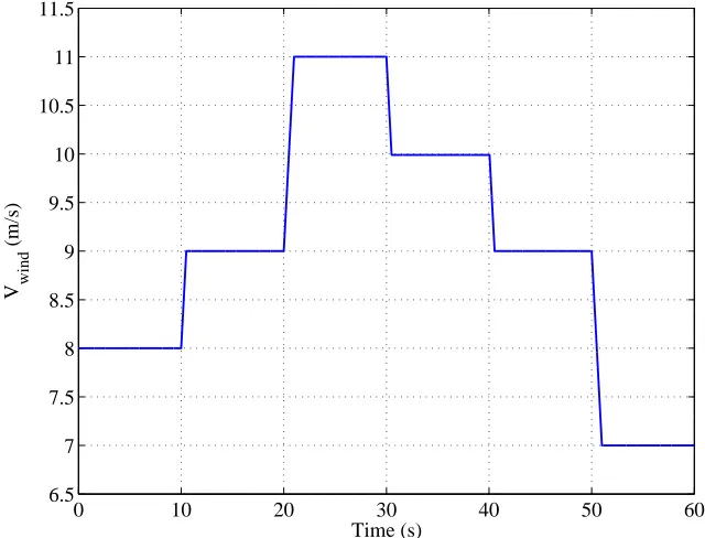
4.4.1 Wind speed with large step changes . . . 75
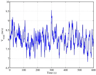
4.4.2 Wind speed with random changes . . . 78
4.4.3 Low-voltage ride through capability . . . 83
4.4.4 Parameter uncertainty . . . 86
4.5 Summary . . . 87
5 Nonlinear Adaptive Control for Maximum Power Point Tracking 91 5.1 Introduction . . . 91
5.2 Problem Formulation . . . 92
5.3 Nonlinear Adaptive Control based on Perturbation Estimation . . . 94
5.3.1 Input-Output linearization . . . 94
5.3.2 Perturbation observer . . . 95
5.3.3 Design of NAC controller . . . 97
5.4 Controller Design . . . 97
5.4.1 With wind speed measurement . . . 97
5.4.2 Without wind speed measurement . . . 100
5.5 Simulation Studies . . . 103
5.5.1 With wind speed measurement . . . 103
5.5.2 Without wind speed measurement . . . 113
5.5.3 Parameter uncertainties . . . 118
5.6 Summary . . . 121
6 Conclusion and Future Work 123 6.1 Conclusion . . . 123
6.2 Future Works . . . 125
References 127
List of Figures
2.1 Schematic diagram of a fixed-speed wind turbine . . . 12
2.2 Schematic diagram of Type B wind turbine . . . 14
2.3 Schematic diagram of Type C wind turbine . . . 15
2.4 Schematic diagram of Type D wind turbine . . . 15
2.5 Drive train models of wind power generation systems . . . 20
2.6 DFIM phase circuits . . . 21
2.7 a-b-ctoα-βaxes transformation of stationary frame . . . 23
2.8 Transformation between stationary reference frames for stator and rotor variables . . . 24
2.9 Park transformation . . . 26
2.10 Transformation of reference frames . . . 26
2.11 Dynamicd-qequivalent circuits of machine . . . 27
2.12 Power converter in DFIG based wind turbine . . . 29
3.1 Power control under stator flux oriented frame . . . 38
3.2 Power control under stator voltage oriented frame . . . 40
3.3 Vector control scheme of grid-side converter . . . 40
3.4 Reference computation of rotor current from stator active and reac-tive power . . . 49
3.5 References of stator active and reactive power . . . 51
3.6 Stator active power regulation by RC & FLC, VC and tracking error 51 3.7 Stator active power regulation by RC & FLC, DPC and tracking error 52 3.8 Stator reactive power regulation by RC & FLC, VC and tracking error 52 3.9 Stator reactive power regulation by RC & FLC, DPC and tracking error . . . 53
3.10 Responses of stator active power under grid disturbance . . . 54
3.11 Responses of stator reactive power under grid disturbance . . . 54
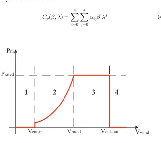
4.1 Wind turbine operation regions . . . 59
4.2 The power coefficientCpversus tip speed ratio at different pitch angles 60 4.3 ψqsmode loci under time-varying wind speed . . . 69
4.4 ψdsmode loci under time-varying wind speed . . . 70
4.6 ψdsmode loci under grid disturbance . . . 72
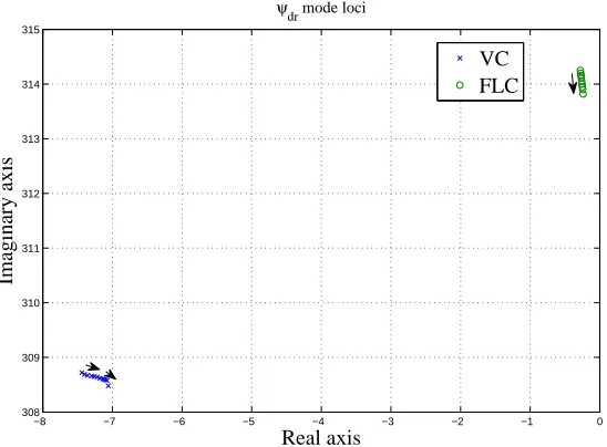
4.7 ψdrmode loci under grid disturbance . . . 72
4.8 ψdsmode loci under parameter uncertainty . . . 73
4.9 ψdrmode loci under parameter uncertainty . . . 74
4.10 Wind speed with large step changes . . . 75
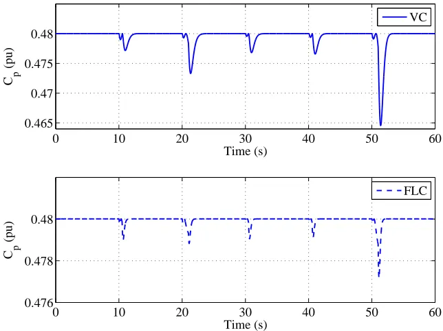
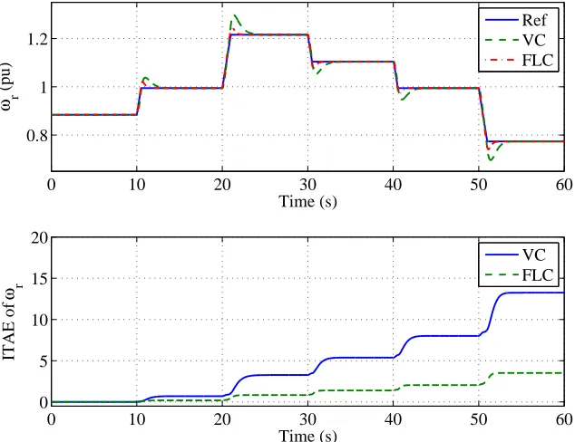
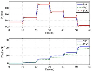
4.11 The power coefficient and its ITAE under the step change of wind speed . . . 76
4.12 The rotor speed and its ITAE under the step change of wind speed . 77 4.13 The electric power and its ITAE under the step change of wind speed 78 4.14 The stator reactive power under the step change of wind speed . . . 79
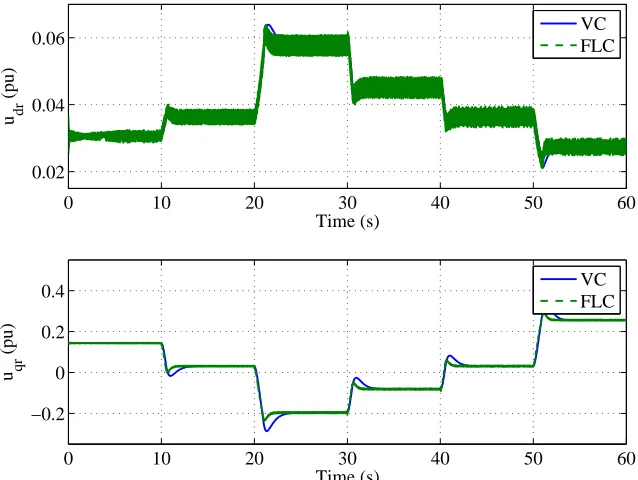
4.15 The rotor voltage ind- andq-axis under the step change of wind speed 79 4.16 Time-varying wind speed . . . 80
4.17 The power coefficient under the random wind speed . . . 81
4.18 The rotor speed under the random wind speed . . . 81
4.19 The electric power under the random speed . . . 82
4.20 The stator reactive power under the random wind speed . . . 82
4.21 The rotor voltage ind- andq-axis under the random wind speed . . 83
4.22 The grid disturbance . . . 84
4.23 The power coefficient under the grid disturbance . . . 84
4.24 The rotor speed under the grid disturbance . . . 85
4.25 The electric power under the grid disturbance . . . 85
4.26 The stator reactive power under the grid disturbance . . . 86
4.27 The time-varying rotor resistance . . . 87
4.28 The power coefficient under the time-varying rotor resistance . . . . 88
4.29 The rotor speed under the time-varying rotor resistance . . . 88
4.30 The electric power under the time-varying rotor resistance . . . 89
4.31 The stator reactive power under the time-varying rotor resistance . . 89
4.32 The rotor voltage ind- andq-axis under the time-varying rotor re-sistance . . . 90
5.1 The typical power versus speed characteristics without wind speed measurement . . . 93
5.2 Control scheme of NAC with wind speed measurement . . . 100
5.3 Control scheme of NAC without wind speed measurement . . . 103
5.4 Step change of wind speed . . . 104
5.5 Power coefficient under step change of wind speed . . . 105
5.6 Response of rotor speed under step change of wind speed . . . 105
5.7 Response of electric power under step change of wind speed . . . . 106
5.8 Response of stator reactive power under step change of wind speed . 106 5.9 Rotor voltage of NAC and FLC ind-axis . . . 107
5.10 Rotor speedωrestimation and estimate error . . . 107
5.11 Perturbation response off1under step change of wind speed . . . . 108
5.12 Stator reactive powerQsestimation and estimate error . . . 108
5.13 Perturbation response off2under step change of wind speed . . . . 109
5.14 Time-varying wind speed . . . 110
5.15 Power coefficient under time-varying wind speed . . . 110
5.16 Response of rotor speed under time-varying wind speed . . . 111
5.17 Response of electric power under time-varying wind speed . . . 111
5.18 Response of stator reactive power under time-varying wind speed . . 112
5.19 Rotor voltage of NAC and FLC ind-axis . . . 112
5.20 Rotor speedωrestimation and estimate error . . . 113
5.21 Perturbation response off1under time-varying wind speed . . . 114
5.22 Stator reactive powerQsestimation and estimate error . . . 114
5.23 Perturbation response off2 under time-varying wind speed . . . 115
5.24 Case of without wind speed measurement . . . 115
5.25 Response of rotor speed without wind speed measurement . . . 116
5.26 Response of electric power without wind speed measurement . . . . 116
5.27 Response of stator reactive power without wind speed measurement 117 5.28 Rotor voltage of NAC and FLC ind-axis without wind speed mea-surement . . . 117
5.29 Electric power errors under uncertainties of rotor resistance . . . 118
5.30 System outputs errors under uncertainties of rotor resistance . . . . 119
5.31 Electric power errors under tower shadow . . . 120
5.32 System outputs errors under tower shadow . . . 120
5.33 Electric power errors under grid voltage dips . . . 121
List of Tables
2.1 Cpcoefficientsαi,j . . . 18
3.1 Control parameters of FLC and proposed controller . . . 50
4.1 Behaviors for different eigenvalues . . . 68
4.2 Eigenvalues under nominal operation point . . . 70
Chapter 1
Introduction
1.1
Background
Wind power, as a clean and sustainable energy, has obtained highly
concentra-tions during the past decade [1], [2]. Research and development of renewable
ener-gy has gained tremendous momentum in the past decade as the cost of conventional
electrical power generation continuously escalate due to the limited fuel resources,
and the general public becomes increasingly concerned of the environmental
im-pacts caused by the thermal and nuclear generation. Among many technologies
promising green power, the utilization of wind energy via wind power generation
system (WPGS) is one of the most mature and well developed. Across the world,
the total capacity of wind generation has already exceeded giga-watt (GW) rating
and larger wind farms are constantly being planned and commissioned [3], [4], [5].
The main components of a WPGS includes the turbine rotor, gearbox, generator,
transformer, and possible power electronics. The turbine rotor converts the
fluctu-ating wind energy into mechanical energy, which is converted into electrical power
through the generator, and then transferred into the grid through a transformer and
transmission line. Wind turbines capture the power from the wind by means of
aerodynamically designed blades and convert it to rotating mechanical power. The
number of blades is normally three and the rotational speed decreases as the radius
1.2 Challenges & Problems 2
be 10-15 rpm. The weight-efficient way to convert the low-speed, high-torque
pow-er to electrical powpow-er is to use a gearbox and a genpow-erator with standard speed. The
gearbox adapts the low speed of the turbine rotor to the high speed of the generator.
The gearbox may be not necessary for multi-pole generator systems.
The generator converts the mechanical power into electrical energy, which is
fed into a grid through a power electronic converter, and a transformer with circuit
breakers and electricity meters. The connection of wind turbines to the grid is
possi-ble at low voltage, medium voltage, high voltage, and even at the extra high voltage
system since the transmittable power of an electricity system usually increases with
increasing the voltage level. While most of the turbines are nowadays connected to
the medium voltage system, large offshore wind farms are connected to the high and
extra high voltage level.
Doubly fed induction generators (DFIG) based wind turbines (DFIG-WT), a
typ-ical employed WPGS, have be widely used to achieve the maximum power
conver-sion, smaller capacity of power electronic devices and full controllability of active
and reactive power of the DFIG [6], due to their characteristics such as varying speed
operation. The stator circuit of the DFIG is connected to the grid directly, while the
rotor circuit is fed via a back-to-back power converter. The back-to-back converter
consists of two converters, i.e., rotor-side converter and grid-side converter, which
are connected ”back-to-back”. Between the two converters a dc-link capacitor is
placed, as energy storage, in order to keep the voltage variations (or ripple) in the
dc-link small.
1.2
Challenges & Problems
1.2.1
Nonlinear dynamics of DFIG-WT
The DFIG-WT is a dynamic system with strong nonlinear coupled
characteris-tics and time varying uncertain inputs. The aerodynamic of wind turbine introduces
strong nonlinearities and uncertainties [28]. Objectives of the wind-turbine
con-troller depend upon the operating area defined via wind speed [29]. For low wind
recommend-1.2 Challenges & Problems 3
ed to limit power production and rotor speed above the rated wind speed to protect
the mechanical part of the WPGS. The power regulation of the wind turbine is a
highly nonlinear system as the plant, actuation and control objectives are all strong
nonlinear [30].
As an induction machine, the DFIG is also a typical nonlinear system as
induc-tion motor, which has been used widely as a test benchmark for nonlinear control
system design. With the time-varying and intermittent wind power input, DFIG-WT
is required to operate at an operation envelope with a wide range rather than one
op-eration point. Moreover, during voltage sags due to grid load disturbances or grid
faults, DFIG-WT will operate far away from its normal operation point. During the
grid fault period and post-fault period, terminal voltage normally dropped close to
the ground and cause the strong dynamics in the stator and rotor currents, and such
that stator-flux will not be remained as constant as well. This will destroy the
condi-tion of the mostly used VC schemes for DFIG-WTs and dynamic of the active and
reactive power of the DFIG are still coupled during the transient period of
stator-flux or stator-voltage. As all vector control schemes depend upon the assumptions
of constant voltage and flux to realize asymptotical decoupling control of the active
and the reactive power, it can expect that their performance will be degraded during
voltage sags and grid faults. On the other side, unlike the vector control of induction
motor in which the rotor flux is controlled directly, stator-flux of the DFIG normally
is not one of the controlled variables and thus not controlled directly.
The control function within the vector control scheme has commonly been
per-formed by using PI controllers. One challenge is how to tune the parameters of
the PI loops to provide optimal performance around one special operation point
and cope with the time-varying operation points. For examples, many results have
been done to automatically tune the PI controller’s parameters, such as using
ge-netic algorithm [42] and particle swarm optimization [43]. Automatic tuning based
on artificial intelligence and gain schedule technique have been proposed to provide
optimal performance for a varying operation condition. Input/output linearization
have been proposed to fully decoupling control of induction motor [50, 85]. When
con-1.2 Challenges & Problems 4
version, rotor speed will travel between the sub-synchronous to super-synchronous
speed and other state variables of the DFIG, including stator and rotor currents and
the rotor voltages, are dynamic variables so as to inject different value of active
power. However, because the system is highly nonlinear, it is difficult to find one set
of parameters, which can provide a consistent optimal response when the operation
point changes. Moreover, in some worst cases, unstable mode may exist because of
one set of PI parameters [45]. Other linear control strategies, such as LQG, which
are designed based a linearized model around a special operation point, may face
d-ifficulties to find approximate gains to maintain optimal efficiency for a wide range
of operation points changing with the varying wind speed, and guaranteeing the
overall system stability when the system operates from sub-synchronous mode to
super-synchronous mode [35].
Compared with linear methods, which are designed based on a linear model
obtained from one operation point, nonlinear control methods can provide
consis-tent optimal performance across the operation envelope rather than at an operation
point and have already attracted lots of research efforts, such as gain schedule
con-trol [31, 32], sliding mode concon-trol [14], multi-variables LQG concon-trol [33], feedback
linearization control (FLC) which assuming exact knowledge of the power
conver-sion coefficient of the wind turbineCp[34] and nonlinear adaptive control with esti-mation of the input wind torque by assuming it as an unknown constant value [35].
Assume the exact knowledge of the wind-turbine power conversionCp function, it is shown that FLC method outperforms gain schedule and LQG methods with less
control efforts and better overall performance.
A fuzzy logic controller can overcome this problem by varying its parameters
according to the operating point; however, it cannot guarantee an optimal response
[46]. An adaptive controller based on estimation of the uncertain plant parameters,
allowing the controller parameters for an optimal response to be adjusted to deal
with account for changing plant dynamics. Thus so far, only a few applications of
adaptive control applied to variable-speed wind turbines have appeared in literature.
Adaptive control algorithms proposed in [47] uses a doubly fed induction generator
1.2 Challenges & Problems 5
circuit and the grid. Using this configuration the generator torque and hence the
turbine speed is changed by adjusting the firing angle of the inverter. A similar
scheme was used in [35], where the excitation voltage across the rotor circuit was
also adjusted.
1.2.2
Uncertain wind power inputs
Variable speed operation of DFIG-WT operates under time-varying uncertain
wind power input, due to time-varying wind speed. Besides the wind turbulence,
tower shadow effect of the horizontal axis wind turbine will also cause periodical
variation on the input wind power, even with constant average wind speed. Most
works do not consider the time-varying characteristics of the wind power at the
designing stage, while validate the effect of the controller to reject the time-varying
wind power via simulation. The wind speed is assuming to be constant such that
the input torque is treated as a constant. A few works are treating it as a
time-varying input. Most adaptive control of WT assumes the input torque as an unknown
constant or slow time-varying and updates it via an estimator, because there is not an
effective method in the control filed to estimate the fast and time-varying unknown
parameters and dynamics. Sliding mode methods treats the time-varying input as
parts of the uncertainties [49].
1.2.3
Fault ride through requirement
With the penetration level of wind energy increased in the current power grid,
fault ride through (FRT) capability has been introduced into most grid codes as one
of the important requirements for the WPGS [15]. The FRT capability, or known
as low voltage ride through (LVRT) capability, specifies that the WPGS must be
connected to the power grid during a grid fault to provide active power control to the
grid during and after the grid fault and to help re-establish the grid voltage after the
clearance of the grid fault. The FRT capability is necessary in integrating large-scale
wind power generations into the power networks, because it reduces the spinning
1.2 Challenges & Problems 6
and stability of the grid.
The FRT is of special interest to DFIG-WT since the stator of the DFIG is
con-nected directly with the grid and is sensitive to voltage sags caused by grid faults
or load disturbances. The voltage sags of the stator will result in a sharp increase
of the stator-flux and over currents of the stator and the rotor windings due to the
magnetic coupling between the stator and the rotor windings. These over currents,
called inrush currents, may be raised up to three times of their rated values and
will damage the rotor and stator windings. And the most serious consequence of
such inrush currents is that they can lead to the breakdown of the rotor-side power
electronic converter. The voltage sags will also yield the fluctuation of the DC-link
voltage, which is controlled via the grid-side converter, and will in turn, affect the
dynamic of the rotor-side converter since the DC voltage is required to be remained
as constant for operation of the rotor-side converter.
Traditionally, the FRT capability of the DFIG-WT is achieved by the installing
crowbar protection of the rotor-side converter [16–18]. However, this solution
can-not avoid the disconnection of the wind turbine with the grid during the fault. A
sudden loss of large-capacity wind power during the fault will introduce frequency
and voltage control problems in the network. Moreover, short-circuit of the rotor
of the DFIG converts the DFIG into a squirrel-cage induction generator and loss
control over the power of the DFIG, which will consume more reactive power and
worsen the voltage sag as the voltage regulation from the power network needs
re-active power support during the fault clearing and after the fault period.
Other two methods of improving the FRT capability are hardware modification
and designing/modifying of the control of the DFIG-WT [19–22]. There is a lots of
efforts on investigating and improving of the LVRT of the DFIG-WT via improving
and designing an advanced controller to limit the peak value of rotor inrush current
and the fluctuation of the dc-link voltage [20–22]. However, most results reported
are based on vector control schemes, which rely on the assumptions of a constant
stator-flux and stator-voltage. Due to the relatively smaller value to the stator
1.2 Challenges & Problems 7
damped system due to a very smallRs/Ls value. These assumptions are not valid during the voltage sags and grid fault conditions since the stator-flux has performed
strong undamped transient dynamic [51]. Moreover, as in most work, stator-flux is
not controlled and thus the performance of the DFIG-WT with VC will be degraded
under grid faults. The VC based on the stator voltage shows similar characteristics.
To improve the FRT capability, control of the dynamic of the stator variables,
stator-flux and stator-voltage, should be considered at the designing stage of the controller.
1.2.4
Voltage and stability support of power networks
WPGSs with large capacity are required to support the operation of the power
networks via providing similar control functionalities as conventional synchronous
generators (SG), such as voltage control, frequency control and stability
improve-ment [23, 24]. Control of the DFIG to make its behavior like an SG was proposed
in [24–26], in which control blocks normally employed in the SG like automatic
voltage regulator (AVR) and power system stabilizer (PSS) are applied to the DFIG,
and a new control scheme called as flux magnitude-angle controller (FMAC) is
ob-tained. In the FMAC, magnitude and angle to the rotor flux are employed as control
variables for terminal voltage and active power, respectively. Compared with the
SG, the DFIG has better controllability to achieve independent control of the
ter-minal voltage and active power (or the provision of damping) because it has two
independent control inputs, while the SG involves a compromise between the
con-flicting requirements of voltage control and the provision of damping as both AVR
and PSS use the magnitude of the field voltage as the control variables (Note that
the angle of voltage field cannot change as it is aligned with the rotor). However, all
additional controllers are designed based on classical linear control theory, and their
parameters are optimized based on one operation point. Based on the idea of the
FMAC and solving the parameter tuning, a damping controller is designed based on
a simple PI controller and tuned using bacterial foraging technique to enhance the
damping of the oscillatory modes [27].
On the other side, because it is difficult to obtain the detailed nonlinear
1.3 Motivations 8
carried out based on a single-machine-infinite-bus (SMIB) system, and then
veri-fy the controller’s performance in the multi-machine power systems via simulation
studies. Interactions with the power networks require that the dynamic of the
pow-er networks must be considpow-ered during the design stage of the controllpow-er, i.e., the
design of the controllers did better be carried out in multi-machine-power-systems.
Decentralised nonlinear control has been proposed for the improvement of transient
stability of a power system, in which terminal voltage of the DFIG and slip speed
are decoupled controlled viad-qcomponents of the rotor voltage [36]. The design is based on a simplified third-order model of the DFIG with stator dynamics ignored,
while the input prime wind power is assumed as constant.
1.3
Motivations
The performance of DFIG-WT depends heavily upon the controllers applied on
the generator side and the wind turbine side. The DFIG-WT is usually controlled via
a cascaded structure including an inner fast-loop for power regulation of the DFIG
and an outer relative slow loop for the speed control of drive train. The reference of
active power of the DFIG is determined based on the maximum energy conversion,
which is defined as maximum power point tracking (MPPT), when wind speed is
below the rated value; while constant reference is given when wind speed is above
the rated value. The wind turbine also employs pitch angle control to regulate the
extracted power from wind source by wind turbine for wind speed above the rated
value, while pitch angle is fixed when wind speed below the rated value.
Main purposes of this thesis are to develop advanced control strategies for
DFIG-WTs to improve the energy conversion efficiency and the transient dynamics of
DFIG-WTs, by considering nonlinear dynamics, uncertain wind power inputs and
grid faults. At first, modeling of a DFIG-WT and the conventional vector control
have been reviewed and prepared for the following research. Then a fully decoupled
power controller is proposed by using nonlinear control to improve the
asymptot-ically decoupled characteristics provided by VCs. Thirdly, nonlinear control has
op-1.4 Thesis Outline 9
erating below the rated wind speed. Both modal analysis and simulation studies
have been carried out. Finally, to improve the robustness of the nonlinear control
and to compensate the time-varying and uncertain wind power inputs, a nonlinear
adaptive control based on perturbation estimation has been studied for the MPPT of
DFIG-WTs.
1.4
Thesis Outline
• Chapter 2 presents the modeling of a doubly fed induction generator based variable-speed wind turbine, including dynamic model of wind turbine, drive
train, DFIG and power electrical converters. For the controller design, the
dynamic model of DFIG is obtained under the two-phase d-q rotating ref-erence frame by applying Clarke and Park’s transformations of the original
three-phase natural reference frame.
• Chapter 3 proposes a nonlinear power control for DFIG. The conventional used power control strategy, vector control, is recalled at first. As vector
con-trol can only achieve the asymptotical regulation of the active/reactive powers
of the DFIG, a fully decoupled nonlinear power control based on feedback
linearization control is designed for the direct power control of the DFIG.
Moreover, a cascade two stages nonlinear controller, which consists of an
outer loop to provide current reference for the rotor current from the stator
ac-tive and reacac-tive powers, and an inner loop applies the input/output feedback
linearization control for the current regulation.
• In Chapter 4, the nonlinear control based maximum power point tracking is studied. The operation regions of wind turbine are introduced at first, where
MPPT control normally works in the range between the cut-in and rated wind
speed. Both VC and FLC are applied for MPPT control under time-varying
wind speeds, to achieve the maximum power extraction from the wind power.
Modal analysis is used to analysis the dynamics of DFIG-WT provided by
1.4 Thesis Outline 10
dynamics with time-varying wind power inputs.
• Chapter 5 investigates the nonlinear adaptive control for DFIG-WT in order to deal with the parameter uncertainties, uncertain wind power inputs and
improve the robustness of the nonlinear controller proposed in Chapter 4. The
proposed adaptive controller designs a perturbation observer to estimate the
real time perturbation and uses it to compensate the real uncertainties and
disturbances. The design includes two cases: with and without wind speed
measurement are carried out, followed by simulation studies.
Chapter 2
Models of a DFIG based Variable
Speed Wind Turbine
This chapter describes models of a wind power generation system equipped with
doubly fed induction generator for variable speed wind turbine. Different typical
configurations of WPGS are reviewed at first. The aerodynamic of wind turbine,
drive train, generator(DFIG), and power electrical converters are investigated
re-spectively. Detailed models of the DFIG based on different reference frames are
given.
2.1
Introduction
Most modern WPGSs use horizontal axis design, three blades and upwind wind
turbines. The larger WTs tend to operate at variable speed whereas smaller, simpler
turbines are of fixed speed. For a fixed-speed wind turbine, the turbulence of the
wind results in power variations, and thus affect the power quality of the grid. As in
a variable-speed wind turbine, the generator is controlled by power electronic
equip-ments, which makes it possible to control the rotor speed to maximize the energy
conversion efficiency. In this way, the power fluctuations caused by wind
variation-s can be abvariation-sorbed by changing the rotor variation-speed. Thuvariation-s power variation originating
2.1 Introduction 12
power quality impact caused by the wind turbine can be improved, compared to a
fixed-speed turbine.
Fixed-speed wind turbines
This type of turbines are also called Type A turbine. Fixed-speed wind turbines
are electrically fairly simple devices consisting of a WT rotor, a low-speed shaft, a
gearbox, a high-speed shaft and an induction (or called as asynchronous)
genera-tor. From the electrical system viewpoint, they are perhaps best considered as large
fan drives with torque applied to the low-speed shaft from the wind flow. Figure
2.1 illustrates the configuration of a fixed-speed wind turbine [37]. It consists of
a squirrel-cage induction generator (SCIG) coupled to the power system through a
turbine transformer. The generator operating slip changes slightly as the operating
power level changes and the rotational speed is therefore not entirely constant.
Be-cause the operating slip variation is generally less than 1%, this type of WPGS is
normally referred to as fixed speed.
SCIG WT
Soft starter Gear
box
Grid
Capacitor bank
transformer
Figure 2.1: Schematic diagram of a fixed-speed wind turbine
Squirrel-cage induction machines consume reactive power and so it is
conven-tional to provide factor correction capacitors for each wind turbine. The function
of the soft-starter unit is to build up the magnetic flux slowly and thus minimize
transient currents during energization of the generator. Meanwhile, by applying the
network voltage slowly to the generator, once energized, it brings the drive train
2.1 Introduction 13
Variable speed wind turbine
During the past few years, variable-speed wind turbines have become the
dom-inant type among the installed wind turbines. Variable-speed wind turbines are
designed to achieve maximum aerodynamic efficiency over a wide range of wind
speeds. With a variable-speed operation, it has become possible continuously to
adapt (accelerate or decelerate) the rotational speed ωr of the wind turbine to the wind speed Vwind. Thus, the tip speed ratio λ can be controlled at a predefined optimal value that corresponds to the maximum power coefficient. Contrary to a
fixed-speed system, the variations in wind are absorbed by changes in the generator
speed. The electrical system of a variable-speed wind turbine is more complicated
than that of a fixed-speed wind turbine. It is typically equipped with an
induc-tion or synchronous generator and connected to the grid through power converters.
The power converters control the generator speed; that is, the power
fluctuation-s caufluctuation-sed by wind variationfluctuation-s are abfluctuation-sorbed mainly by changefluctuation-s in the rotor fluctuation-speed of
generator and consequently in the rotor speed of wind turbine. The advantages of
variable-speed wind turbines are an increased energy capturing efficiency, improved
power quality and reduced mechanical stress on the wind turbine. The
disadvan-tages are losses in power electronics converters, the use of more components and
the increased cost of equipment and maintenance because of the power
electronic-s. The introduction of variable-speed wind-turbine types increases the number of
applicable generator types and also introduces several degrees of freedom in the
combination of generator typed and power converter type [38].
Most common used variable speed wind turbine configurations are listed as
fol-lows.
a Limited variable speed (Type B)
b Variable speed with partial scale frequency converter (Type C)
c Variable speed with full scale frequency converter (Type D)
Figure 2.2 shows the schematic diagram of a type B wind turbine. This
configu-ration corresponds to the limited variable speed wind turbine with a variable
2.1 Introduction 14
used by the Danish manufacturer Vestas since mid 1990s. The generator is directly
connected to the grid. A capacitor bank performs the reactive power compensation.
A smoother grid connection is achieved by using a soft-starter. The unique feature
of this concept is that it has a variable additional rotor resistance, which can be
changed by an optimally controlled converter mounted on the rotor shaft. Thus, the
total rotor resistance is controllable. This optical coupling eliminates the need for
costly slip rings that need brushes and maintenance.
WRIG WT
Soft starter Gear
box
Grid
Capacitor bank
transformer Variable
resistance
Figure 2.2: Schematic diagram of Type B wind turbine
The rotor resistance can be changed and thus the slip is controlled to regulate
the power output of the WPGS. The range of the speed control depends on the
size of the variable rotor resistance. Typically, the speed range is from 0 to10 %
above synchronous speed. Wallace and Oliver (1998) describe an alternative concept
by using passive components instead of a power electronic converter, which can
achieves a10% slip range.
For type C wind turbine, the schematic diagram is shown in Figure 2.3. This
configuration, known as DFIG-WT, corresponds to the limited variable speed wind
turbine with a DFIG and partial scale frequency converter (rated at approximately
30% of the generator capacity) on the rotor circuit. The partial scale frequency
con-verter performs the reactive power compensation and the smoother grid connection.
It has a wider range of dynamic speed control compared with that of type B wind
turbine, depending on the size of the frequency converter. Typically, the speed range
2.1 Introduction 15
makes this concept attractive from an economical point of view. Compared with
type B, its main drawbacks are the use of slip rings and protection of the converters
in the case of grid faults.
WRIG
WT
Gear box
Grid transformer
Partial scale frequency converter
Figure 2.3: Schematic diagram of Type C wind turbine
The type D wind turbine corresponds to a fully variable speed wind turbine, with
the generator connected to the grid through a full-scale frequency converter. The
grid-side frequency converter performs the reactive power compensation and the
smoother grid connection. The generator can be excited electrically (WRSG/WRIG)
or by a permanent magnet (PMSG). Some fully variable-speed wind turbine systems
have no gearbox. In these cases, a direct driven multi pole generator with a large
diameter is used. The wind turbine companies Enercon, Made and Lagerwey are
examples of manufacturers using this configuration.
WRIG/WRSG/PMSG
WT
Gear box
Grid transformer
Power electronics converter
2.2 Aerodynamics of Wind Turbines & Drive Train Model 16
2.2
Aerodynamics of Wind Turbines & Drive Train
Model
Wind turbines produce electricity by converting the mechanical power of the
wind to drive an electrical generator. Wind passes over the blades, generating lift and
exerting a turning force. The rotating blades turn a shaft inside the nacelle, which
goes into a gearbox. The gearbox increases the rotational speed to an appropriate
value for the generator, which uses magnetic fields to convert the mechanical energy
into electrical energy.
The power contained in the wind is given by the kinetic energy of the flowing
air mass per unit time [39]. That is
Pair =
1 2ρπR
2V3
wind (2.2.1)
wherePairis the power contained in wind (in W),ρis the air density (1.225 kg/m2at 15 degree and normal pressure),Ris the blade length (in m), andVwind is the wind velocity (in m/s) without rotor interference, i.e., ideally locating at infinite distance
from the rotor.
The power captured by the wind turbine Pm is given by the power conversion coefficient
Cp =
Pm
Pair
(2.2.2)
Pm =Pair×Cp =
1
2CpρπR 2V3
wind (2.2.3)
whereCp is the power conversion coefficient.
A maximum value ofCp is defined by the Betz limit, which states that a turbine can never extract more than0.593of the power from an air stream. In reality, wind turbine haveCpvalues in the range0.25-0.45.
For a given wind turbine, the coefficientCp is dependent upon the aerodynamic characteristic of the wind turbine, and a complex nonlinear function of the blade tip
speed ratioλ= ωrR
2.2 Aerodynamics of Wind Turbines & Drive Train Model 17
and pitch angles. Based on experimental results, curve fitting technique can be used
to obtain the formula ofCp. Curve fitting was performed to obtain the mathematical representation of theCpcurves used in the model: [40]:
Cp(β, λ) =
4 X
i=0 4 X
j=0
αi,jβiλj (2.2.4)
where the coefficientαi,jare given in Table 2.1.
Note thatCp is a nonlinear formulation ofλandβand it is not very accurate for very low and very big wind speed. Moreover,Cp’s value will vary with changes of the shape of the blade caused by ageing and ices mounted on the blade.
Model of Drive Train
The mechanical representation of the entire wind turbine is complex. The power
transmission train is constituted by the blades linked to the hub, coupled to the slow
shaft, which is linked to the gearbox, which multiplies the rotational speed of the
fast shaft connected to the generator.
The mechanical elements of a wind turbine and the forces suffered or transmitted
through its components are very numerous. It is therefore necessary to choose the
dynamics to represent and the typical values of their characteristic parameters. The
first is the resonant frequency of the power train. For the purpose of the control
design and simulation, representing the fundamental resonance frequency of the
drive train is sufficient and a two-mass model, can then be used to represent the
dynamic of the drive train. The second order resonance frequency is much higher
and its magnitude is lower and thus can be ignored. The following two types of
drive train models of the WPGS are usually available in the power system analysis,
as shown in Figure 2.5.
In Figure 2.5(a), the two-mass model of drive train can be described by: [41]
2Ht
dωt
dt =Tm−Dtωt−Dtg(ωt−ωr)−Ttg 2Hg
dωr
dt =Ttg+Dtg(ωt−ωr)−Dgωr−Te dTtg
dt =Ktg(ωt−ωr)
2.2 Aerodynamics of Wind Turbines & Drive Train Model 18
Table 2.1: Cpcoefficientsαi,j
i j αi,j
4 4 4.9686e-010
4 3 -7.1535e-008
4 2 1.6167e-006
4 1 -9.4839e-006
4 0 1.4787e-005
3 4 -8.9194e-008
3 3 5.9924e-006
3 2 -1.0479e-004
3 1 5.7051e-004
3 0 -8.6018e-004
2 4 2.7937e-006
2 3 -1.4855e-004
2 2 2.1495e-003
2 1 -1.0996e-002
2 0 1.5727e-002
1 4 -2.3895e-005
1 3 1.0683e-003
1 2 -1.3934e-002
1 1 6.0405e-002
1 0 -6.7606e-002
0 4 1.1524e-005
0 3 -1.3365e-004
0 2 -1.2406e-002
0 1 2.1808e-001
2.3 Dynamic Model of DFIG 19
where ωt and ωr are the turbine and generator rotor speed, respectively; Tm and
Te are the mechanical torque applied to the turbine and the electrical torque of the generator, respectively; Ttg is an internal torque of the model; Ht and Hg are the inertia constants of the turbine and the generator, respectively; Dt and Dg are the damping coefficients of the turbine and the generator, respectively;Dtgis the damp-ing coefficient of the flexible coupldamp-ing between the two masses; Ktg is the shaft stiffness.
To simplify the analysis, the drive train system can also be modeled as a single
lumped-mass system with a lumped inertia constantHmas in Figure 2.5(b):
Hm =Ht+Hg (2.2.6)
Therefore, one-mass model of drive trains is given by
2Hm
dωr
dt =Tm−Te−Dmωr (2.2.7)
whereDmis the damping of the lumped-mass system.
2.3
Dynamic Model of DFIG
Nowadays doubly fed induction machine has been widely used in WPGS. These
types of machines can be used resolutely as a generator or a motor. Though demands
as motor is less because of its mechanical wear at the slip rings but they have gained
their prominence for generator application in wind and hydro power plant because
of its obvious adoptability capacity and nature of controllability of power. In this
section, detailed model of DFIG has been given.
2.3.1
State space model in the
a
-
b
-
c
natural frame
The DFIM is provided with laminated stator and rotor cores with uniform slots
in which three-phase winding are placed as shown in Figure 2.6. Usually, the rotor
winding is connected to copper slip-rings. Brushes on the stator collect the rotor
2.3 Dynamic Model of DFIG 20
t
t
D
T
mtg
T
,
tg tg
K
D
e
T
r
g
D
H
gt
H
( )
a
m
m
D
m t g
H
H
!
H
m
T
T
e( )
b
2.3 Dynamic Model of DFIG 21
as
i
as
u
rr
cr
i
br i ar i
ar
u
br
u ucr
bs
i
cs
i
bsu
cs
u
2.3 Dynamic Model of DFIG 22
of slip-ring-brush system are lumped into rotor phase resistances, and the
convert-er is replaced by an ideal controllable voltage source. The three-phase model of a
DFIG can be described as:
uas =
dψas
dt +iasRs ubs =
dψbs
dt +ibsRs ucs =
dψcs
dt +icsRs
(2.3.1)
uar =
dψar
dt +iarRr ubr =
dψbr
dt +ibrRr ucr =
dψcr
dt +icrRr
(2.3.2)
whereias, ibs,ics are the three-phase stator currents;iar, ibr,icr are the three-phase rotor currents;uas, ubs, ucs are the three-phase stator voltages;uar, ubr,ucr are the three-phase rotor voltages;ψas,ψbs,ψcsare the three-phase stator flux linkages;ψar,
ψbr, ψcr are the three-phase rotor flux linkages; Rs and Rr are stator and rotor re-sistances. Note that, the stator equations are represented in the stator natural frame,
and the rotor equations are described in the rotor natural frame.
2.3.2
Clarke transformation
Considering a symmetrical three phase induction machine with stationary a -phase,b-phase andc-phase axes are placed at120◦angle to each other, as shown in Figure 2.7. The main aim of a Clarke transformation is to transform the three-phase
stationary frame variables into a two-phase stationary frame variablesα-β,and vice versa.
Any three-phase voltage or currentxina-b-ccomponents can be converted into
2.3 Dynamic Model of DFIG 23
,
a
sx
x
sx
b
c
Figure 2.7:a-b-ctoα-β axes transformation of stationary frame
xα xβ x0
=TC
xa xb xc (2.3.3)
whereTC is the transformation matrix of Clarke transformation,
TC =
2 3
0 −1 2 −
1 2 0 √23 −√23
1 2 1 2 1 2 (2.3.4)
x0 is the zero sequence component, which equals to zero for symmetrical three-phase variable. For example, the reference transformation of stator and rotor
cur-rents are described as follows, and the reference frames can be seen in Figure 2.7.
iαs iβs i0s
=TC
2.3 Dynamic Model of DFIG 24
r s
s r
r
Figure 2.8: Transformation between stationary reference frames for stator and rotor variables
iαr
iβr
i0r
=TC
iar
ibr
icr
(2.3.6)
where i0s and i0r are the zero sequence components of stator and rotor current, respectively.
The rotor variables represented in the rotor stationary reference frame can be
referred to the stator stationary reference frame by a transformation matrixTθr, as shown in Figure 2.8.
" is
αr
is βr
# =Tθr
" iαr
iβr
#
(2.3.7)
where
Tθr =
"
cosθr −sinθr
sinθr cosθr
#
(2.3.8)
Note that, for simplified representation, the followingiαr andiβr are described for the rotor current vectors referred to the stator stationary reference frame, like in
2.3 Dynamic Model of DFIG 25
2.3.3
Park transformation
A Park transformation transfer variables from a two-phase stator stationary
ref-erence frame to a two-phase rotating refref-erence frame through the rotation
transfor-mation matrixTP(θ), as shown in Figure 2.9(b).
" ids
iqs
#
=TP(θ)
" iαs
iβs
#
(2.3.9)
whereTP(θ)is the transformation matrix,
TP(θ) =
"
cosθ −sinθ sinθ cosθ
#
(2.3.10)
whereθis the angle betweend-axis andα-axis.
The same transformation in general orthogonal coordinates, rotating at genetic
electric speedω = dθ
dt, is valid for all currents and flux linkages. The transformation from three-phase (a-b-c) to two-phase stationary reference frame (α-β) and to a two-phase rotating reference frame (d-q) is summarized in Figure 2.10.
For the design of controllers, the stator and rotor equations should be referred
to the same reference frame. The stator equations in the stator stationary reference
frameαs-βs can be derived from (a-b-c) three-phase model (2.3.1) by using Clarke transformationTC:
uαs =Rsiαs+
dψαs
dt uβs=Rsiβs+
dψβs
dt
(2.3.11)
where iαs and iβs are α-axis andβ-axis stator currents, respectively; ψαs and ψβs areα-axis andβ-axis stator-flux linkages, respectively.
When the state variables in Eq.(2.3.11) are aligned with the rotatingd-qframe by substituting the Park transformation matrixTP(θ)into Eq.(2.3.11), after the compu-tations of each variables from stationary to rotating reference frame, the equations
can be written as:
uds =Rsids +
dψds
dt −ωψqs uqs =Rsiqs+
dψqs
dt +ωψds
2.3 Dynamic Model of DFIG 26
r
r
!
"
d
q
!
s
r r
s
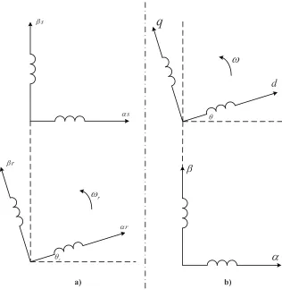
[image:38.595.144.460.105.438.2]a) b)
Figure 2.9: Park transformation
a
b
c
s
s d
q
Clarke Transformation
C
T
Park Transformation
( )
P
T
Stator and rotornatural reference frame
Stator stationary reference frame
s
r
s
r
Rotor stationary reference frame
r
T
Rotating reference frame
2.3 Dynamic Model of DFIG 27
s u
s i
s j !
s
R Lls Llr Rr j( !" r) r
r
i
r u
s Lm r
Figure 2.11: Dynamicd-qequivalent circuits of machine
where all the variables are in rotating reference frame,ωis the rotation speed. The last terms in equation (2.3.12) can be defined as speed emf due to rotation of the
axes, that is, whenω = 0, the equations revert to stationary form.
Since the rotor actually moves at speedωragainst to the stator, the d-q axes fixed on the rotor move at a speedω−ωr. Therefore, in d-q frame, the rotor equations represented in thed-qframe as:
udr =Rsidr+
dψdr
dt −(ω−ωr)ψqr uqr =Rsiqr+
dψqr
dt + (ω−ωr)ψdr
(2.3.13)
Figure 2.11 shows the equivalent circuits for d-q dynamic model that satisfy
equations (2.3.12) and (2.3.13), in which us = uds +juqs, the is, ir, ψs, ψr can be presented in the same form, Ls = Lls+Lm is the stator self-inductance; Lr =
Llr+Lm is the rotor self-inductance;Llsis the stator leakage inductance;Llris the rotor leakage inductance;Lmis the mutual inductance.
The flux linkage expressions in terms of the currents can be obtained from Figure
2.11 as follows:
ψds =Lsids+Lmidr
ψqs =Lsiqs+Lmiqr
ψdr =Lridr +Lmids
ψqr =Lriqr+Lmiqs
2.4 Model of Grid-side Converter and DC-link 28
The electromagnetic torque equation is represented as
Te =ψdsiqs−ψqsids =Lm(iqsidr−idsiqr) = ψdriqr−ψqridr (2.3.15)
In summary, the model of DFIG under d-q rotating reference frame can be obtained by applying Clarke and Park transformations from equations (2.3.1) and
(2.3.2):
dψds
dt =uds−Rsids+ωψqs dψqs
dt =uqs−Rsiqs−ωψds dψdr
dt =udr−Rridr+ (ω−ωr)ψqr dψqr
dt =uqr−Rriqr−(ω−ωr)ψdr
(2.3.16)
The speed ω of above model may take arbitrary value and result in conversion among different reference frames: stator stationary reference frame (ω = 0), rotor stationary reference frame (ω = ωr), synchronous rotating reference frame (ω =
ωs), whereωsis synchronous speed.
The active and reactive stator power equations are presented as:
Ps =udsids +uqsiqs
Qs =uqsids−udsiqs
(2.3.17)
with the mathematical equations for computing the active and reactive powers
of rotor side
Pr=udridr +uqriqr
Qr =uqridr−udriqr
(2.3.18)
2.4
Model of Grid-side Converter and DC-link
As shown in Figure 2.12, the power converter is made up of a back-to-back
converter connecting the rotor circuit and the grid, which is known as a Scherbius
scheme. The converters are typically made of voltage-fed current regulated
2.4 Model of Grid-side Converter and DC-link 29
Rotor-side converter
DC-link chopper
DC-link capacitor
Grid-side converter
Rotor-side filter
Grid-side filter
Figure 2.12: Power converter in DFIG based wind turbine
IGBTs provided with freewheeling diodes (see Figure 2.12). An LC-filter is
pro-vided on each converter output to minimize switching harmonics and to protect
component insulation.
The power rating of the rotor-side converter is dictated by two factors, namely
maximum slip power and reactive power control capability. The rotor-side
convert-er can be seen as a current controlled voltage source convconvert-ertconvert-er. The rotor current
can be controlled in several ways. The commonly used method is by utilizing a
P-WM modulation as presented in [6], [52]. Another option is to employ a hysteresis
modulation method to the rotor-side converter [53]. The principle is also referred
to as current-regulated modulation with a tolerance band control [54] or an adaptive
current control PWM [55]. In this method, the current control tracks the phase rotor
current to be within the hysteresis band by turning on the upper or lower valves of
the converter based on a hysteresis control. When the rotor phase current exceeds
the upper band, the lower valve of the corresponding phase is turned on and the
up-per valve is turned off. Similarly, when the actual current is below the lower band,
the upper valve of the corresponding phase is turned on and the lower valve is turned
off. This mechanism, in turn, forces the actual current to follow the current
2.4 Model of Grid-side Converter and DC-link 30
the switching frequency limitations and the switching losses of the IGBTs [56].
The power rating of the grid-side converter is mainly dictated by maximum slip
power since it usually operates at a unity power factor. A typical output voltage of
the gride-side converter is 480 V [57].
The grid-side converter is normally dedicated to control the dc-link voltage and
reactive power exchange between DC-link and the grid. It can also be utilized to
support grid reactive power during a fault [58] and to enhance grid power
qual-ity [59]. However, these abilities are seldom utilized since they require a larger
converter rating. In stability studies, it is well accepted to disregard the switching
dynamics of the converter and treat them as an ideal device. In addition, converters
are assumed to be able to follow the demanded values of the converter current fast
enough [60].
A detailed model of a grid-side converter presented in [6] is recalled, where
the converter is modeled as a current-controlled voltage source. This constitutes a
representation of the dc-link capacitor and the grid-side filter in the model.
The ac-side circuit equation of the GSC can be written as
digabc
dt =− Rg
Lg
igabc+
1 Lg
(ugabc−usabc) (2.4.1) whereigabc, ugabc, usabc are the grid-side current, voltage and stator voltage in vec-tors, respectively;RgandLgare the reactance and inductance of grid-side converter. By substituting the Clarke and Park transformation matrix Eq. (2.3.4) and (2.3.10)
into Eq. (2.4.1), the equation of the GSC will be represented in the rotating
refer-ence frame. After that, aligning thed-axis of the state variables with the grid voltage vectorus (uds = us, uqs = 0), the followingd-q vector model can be obtained for modeling the GSC ac-side:
udg =Rgidg+Lg
didg
dt −ωsLgiqg+us uqg =Rgiqg +Lg
diqg
dt +ωsLgidg
(2.4.2)
Neglecting harmonics due to switching and the losses in the GSC, the filtering
inductor and the transformer, the power balance equation can be obtained as
PDC =Pr−Pg =CuDC
duDC
2.5 Summary 31
wherePris the active power at the AC terminal of the rotor-side converter;Pg is the active power at the AC terminal of the grid-side converter;PDC is the active power of DC link. These are given by
Pr =udridr+uqriqr (2.4.4)
Pg =udgidg+uqgiqg (2.4.5)
PDC =uDCiDC (2.4.6)
whereidr andiqrare the d and q axis rotor currents, respectively;idq andiqgare the d and q axis currents of grid-side converter, respectively;udq anduqgare the d and q axis voltages of grid-side converter, respectively;vDC is the capacitor DC voltage;
iDC is the current of the capacitor.
2.5
Summary
In this chapter, different topologies of wind turbine generation system were
re-viewed. Types of variable-speed wind turbines are implemented in the current wind
power generation system more frequently than fix-speed wind turbine, as the wind
power output is time-varying and uncertainty. Thereby, the control design for
dif-ferent objectives will be worked out, base on the variable-speed wind turbine with a
doubly-fed induction generator in this thesis.
As follows, the dynamic modeling of drive train was investigated, and the
one-mass lumped model of drive train run through the following studies. The detailed
model of the DFIG system was also studied, with the Clarke and Park
transforma-tions. By apply the transformations, the state variables of the DFIG system can
be transformed into the two-phase vectors oriented with different rotating reference
frame, for simply controller design.
Finally, the dynamic of the DC-link capacitor and the grid-side converter
con-sidering the output filter were investigated for the studies on the control of grid-side
Chapter 3
Nonlinear Power Control of DFIG
based Wind Turbine
3.1
Problem Description
Currently, variable speed WPGSs are continuously increasing their market share,
since they are capable of tracking the wind speed variations by adapting the shaft
speed, and thus, achieving the optimal power generation. The mostly used WPGS
are based on DFIG, which stator is connected to the grid directly and rotor connects
through back to back converters. The major advantage of these facilities lies in
the fact that the power rate of the inverters is around the 25-30 % of the nominal
generator power.
The conventional control method for DFIG is vector control in whichd-q com-ponents of rotor currents are directly linked with stator active power/reactive power
(or torque/flux) and thus the current components can be used to control the stator active and reactive power, respectively, by transforming all variables into a
refer-ence frame fixed to stator flux vector (or voltage vector) [61], [62]. Regarding to
this method, an accurate synchronization with the stator flux vector enables a
3.1 Problem Description 33
frame transforms enables the vector control to treat the state variables of the machine
as DC signals. This feature has resulted in its implementation in most DFIG-WTs,
though the tuning of the controller parameters is not an easy job.
Another drawback of the vector control is several transformations involved, as
well as the heavenly dependence with the stator flux position measurement or
es-timation. Moreover, this method also requires accurate value of machine
parame-ters such as resistances and inductances and nonlinear operation of the DFIG is not
considered for tuning current controllers. Then performance of the vector control
method is affected by changing machine parameters and operation condition.
In [53], DFIG control mechanisms are reported using the stator-flux-oriented
frame with the position of the stator-flux space estimated through the measurement
of the stator-flux space vector inα-βreference frame. In [63], a stator-flux-oriented DFIG control strategy is proposed, in which the position of the stator-flux space
vec-tor is estimated through the measurements of stavec-tor voltage and rovec-tor-current space
vectors inα-β reference frame. In [64], a stator-flux-oriented control of a cascaded doubly-fed induction machine is proposed, in which one of the main approaches
used to estimate the position of stator flux space vector is to add a delay angle
of 90o to the stator voltage space vector. Other control approaches are also
pro-posed recently, such as direct-power-control strategies using the stator-flux-oriented
frame [11], [12].
The modeling of DFIG-WT used for conventional power control have been
rep-resented in the synchronous rotating reference frame as
dψds
dt =uds−Rsids+ωsψqs dψqs
dt =uqs−Rsiqs−ωsψds dψdr
dt =udr−Rridr+ (ωs−ωr)ψqr dψqr
dt =uqr−Rriqr−(ωs−ωr)ψdr