arXiv:1809.01688v1 [math.NT] 5 Sep 2018
OLEG KARPENKOV, MATTY VAN-SON
Abstract. In this paper we introduce generalised Markov num-bers and extend the classical Markov theory for the discrete Markov spectrum to the case of generalised Markov numbers. In particu-lar we show recursive properties for these numbers and find corre-sponding values in the Markov spectrum. Further we construct a counterexample to the generalised Markov uniqueness conjecture. The proposed generalisation is based on geometry of numbers. It substantively uses lattice trigonometry and geometric theory of continued numbers.
Contents
1. Introduction 2
2. Continued fractions and lattice geometry 7
2.1. Regular continued fractions 7
2.2. Basics of lattice geometry 8
2.3. Continuants and their relations to integer sines 9 3. Perron Identity: general theory of Markov spectrum 10 3.1. Generic arrangements and their LLS sequences 10
3.2. Generic reduced forms 12
3.3. Marked LLS sequences and reduced generic arrangements 12 3.4. Perron Identity in one diagram 13 4. Theory of Markov spectrum for integer forms 15
4.1. Reduced matrices 15
4.2. Extremal reduced forms, extremal reduced matrices,
extremal even sequences 18
4.3. Theory of Markov spectrum for integer forms in one
diagram 18
5. Triple-graphs: definitions and examples 21
5.1. Definition of triple-graphs 22
5.2. Farey triples, Farey coordinates for triple-graph structure 23
Date: 04 September 2018.
Key words and phrases. Geometry of continued fractions, Perron Identity, binary quadratic indefinite form.
O. Karpenkov is partially supported by EPSRC grant EP/N014499/1 (LCMH).
5.3. Markov triple-graph 23 5.4. Triple-graphs of finite sequences 24
5.5. Triple-graphs of matrices 24
5.6. Tree structure of G⊕(µ, ν) and G• Mµ, Mν
24 5.7. Reconstruction of triples in the triple-graphs by their
central elements 29
6. Markov tree and its generalisations 30 6.1. Classical Markov theory in one diagram 30
6.2. Markov LLS triple-graphs 32
6.3. Generalised Markov and almost Markov triples 34 6.4. Generalised Markov theory in one diagram 36 6.5. Uniqueness conjecture for Markov triples 37 6.6. A counterexample to the generalised uniqueness conjecture 38
7. Related theorems and proofs 39
7.1. Concatenation of sequences and global minima of the
corresponding forms 39
7.2. Recurrence relation for extended Markov trees 44
7.3. Partial answer to Problem 2 47
References 48
1. Introduction
In this paper we develop a geometric approach to the classical ory on the discrete Markov spectrum in terms of the geometric the-ory of continued fractions. We show that the principles hidden in the Markov’s theory are much broader and can be substantively extended beyond the limits of Markov’s theory. The aim of this paper is to intro-duce the generalisation of Markov theory and to make the first steps in its study.
Markov minima and Markov spectrum. Let us start with some classical definitions. Traditionally the Markov spectrum is defined via certain minima of binary quadratic forms (see [31, 32]). Let us define the Markov minima first.
Definition 1.1. Let f be a binary quadratic form with positive dis-criminant. The Markov minimum of f is
m(f) = inf
Z2\{(0,0)}|f|.
Definition 1.2. Let f be a binary quadratic form with positive dis-criminant ∆(f). The normalised Markov minimum of f is
M(f) = pm(f) ∆(f). The set of all possible values for
1 M(f) is called the Markov Spectrum.
The functional M has various interesting properties. In particular if two forms f1 and f2 are proportional then their normalised Markov minima are the same. The lattice preserving linear transformations of the coordinates also do not change the value of the normalised Markov minima.
By that reason, M(f) depends only on the integer type (see Defini-tion 2.4 below) of the arrangement of two lines forming the locus of f, which has an immediate trace in geometry of numbers.
Some history and background. The smallest element in the Markov spectrum is √5. It is defined by the form
x2+xy−y2
and therefore it is closely related to the golden ratio in geometry of numbers. The first elements in the Markov spectrum in increasing order are as follows:
√
5, √8,
√ 221
5 ,
√ 1517
13 ,
√ 7565 29 , . . .
The first two elements of the Markov spectrum were found in [28] by A. Korkine, G. Zolotareff. It turns out that the Markov spectrum is discrete at the segment [√5,3] except the element 3. This segment of Markov spectrum was studied by A. Markov in [31, 32]. We discuss his main results below.
The spectrum above the so-called Freiman’s constant
F = 2221564096 + 283748
p
462)
491993569 = 4.527829. . .
Remark 1.3. Note that most of the generalised Markov and almost Markov trees are entirely contained in the Markov spectrum above 3, which evidences the fractal nature of the spectrum.
The Markov spectrum has connections to different areas of math-ematics, let us briefly mention some related references. Hyperbolic properties of Markov numbers were studied by C. Series in [34]. A. Sor-rentino, K. Spalding, and A.P. Veselov have studied various properties of interesting monotone functions related to the Markov spectrum and the growth rate of values of binary quadratic forms in [36] and [35, 37]. B. Eren and A.M. Uluda˘g have described some properties of Jimm for certain Markov irrationals in [13]. In his paper [17] D. Gaifulin stud-ied attainable numbers and the Lagrange spectrum (which is closely related to Markov spectrum).
Finally let us say a few words about the multidimensional case. One can consider a form of degree d in d variables corresponding to the product ofdlinear factors. The Markov minima and thed-dimensional Markov spectrum here are defined as in the two-dimensional case. It is believed that thed-dimensional Markov spectrum for d >2 is discrete, however this statement has not been proven yet. We refer the interested reader to the original manuscripts [8, 9, 10, 11, 12] by H. Davenport, and [39] by H.P.F. Swinnerton-Dyer, and to a nice overview in the book [19] by P.M. Gruber and C.G. Lekkerkerker.
Markov numbers and their properties. Let us recall an important and surprising theorem by A. Markov [31, 32] which relates the Markov Spectrum below 3 to certain binary quadratic forms and solutions to the Markov Diophantine equation
x2+y2+z2 = 3xyz.
Definition 1.4. The solutions of this equation are calledMarkov triples. Elements of Markov triples are said to be Markov numbers.
Markov triples have a remarkable structure of a tree. This is due to the following three facts:
Fact 1. If (a, b, c) is a solution to the Markov Diophantine equation then any permutation of (a, b, c) is a solution as well.
Fact 2. If (a, b, c) is a solution to the Markov Diophantine equation then the triple (a,3ab−c, b) is a solution as well.
(1,1,1) (1,2,1) (2,5,1)
(29,433,5) (5,29,2)
(29,169,2) (13,194,5) (5,13,1)
[image:5.612.139.479.91.268.2](34,89,1)
Figure 1. The first 5 levels in the Markov tree.
Let us order the elements in triples (a, b, c) as follows: b ≥ a ≥ c and denote them by vertices. We also connect the vertex (a, b, c) by a directed edge to the vertices (a,3ab−c, b) and (b,3bc−a, c) Then we have an arrangement of all the solutions as a graph which is actually a binary directed tree with the “long” root, see in Figure 1.
The following famous Markov theorem links the triples of the Markov tree with the elements of the Markov spectrum below 3 by means of indefinite quadratic forms with integer coefficients.
Theorem 1.5. (A. Markov [32].) (i) The Markov spectrum below
3 consists of the numbers √9m2−4/m, where m is a positive integer such that
m2+m21 +m22 = 3mm1m2, m2 ≤m1 ≤m, for some positive integers m1 and m2.
(ii)Let the triple (m, m1, m2)fulfill the conditions of item (i). Suppose that u is the least positive residue satisfying
m2u≡ ±m1 mod m and v is defined from
u2+ 1 =vm. Then the form
fm(x, y) =mx2+ (3m−2u)xy+ (v−3u)y2
numbers (here H. Cohn used the trace identity of [15] by R. Fricke). As we show later (see Remark 4.3), the idea of Cohn matrices can be also extended to the case of generalised Markov and almost Markov trees, although the trace rule does not have a straightforward generalisation.
Main objectives of this paper. The generalisation of the classi-cal Markov theory on the discrete Markov spectrum consists of the following major elements.
• First of all we introduce a geometric approach to the classical theory. (The outline see Diagram in Figure 6.) This approach is based on interplay between continued fractions and convex geometry of lattice points in the cones.
• Basing on lattice geometry related to the classical case we con-struct generalised almost Markov and Markov triples of num-bers (see Section 6.3).
• Further we relate generalised Markov triples to the elements of the Markov spectrum. We find Markov minima for the forms related to the generalised Markov trees in Corollary 7.11. • Our next goal is to study the recursive properties of generalised
Markov numbers (Corollary 7.19). These properties are essen-tial for fast construction of the generalised Markov tree (the classical Markov tree is constructed iteratively by the formula of Fact 2 above).
• Finally we collect the main properties of the generalised Markov trees in Theorem 6.20 (see also the diagram in Figure 8). • We produce counterexamples for one of the generalised
unique-ness conjectures, see Examples 6.27 and 6.28.
Organisation of the paper. We start in Section 2 with the definition of continued fractions and a discussion of lattice geometry techniques related to continued fractions.
Section 3 is dedicated to the classical Perron Identity. Our goal here is to relate the following objects: elements of the Markov spectrum, LLS sequences, reduced arrangements, and reduced forms.
In Section 5 we introduce an important general triple-graph struc-ture which perfectly fits to Markov theory and its generalisation pro-posed in this paper. After briefly defining triple-graphs in Subsec-tion 5.1 we show several basic examples of triple-graph structure for Farey triples, Markov triples, triples of finite sequences, and triples of SL(2,Z)-matrices (we refer to Subsections 5.2, 5.3, 5.4, and 5.5 respec-tively). Finally we study several important lexicographically monotone and algorithmic properties of these triple graphs. in Subsections 5.6 and 5.7.
We introduce the extended theory of Markov theory in Section 6. After a brief discussion of the classical case in Subsection 6.1 we for-mulate the main definitions and discuss the extended Markov theory in Subsections 6.2 and 6.3. We show the diagram for the extended Markov theory in Subsection 6.4 (see Theorem 6.20). Finally in Subsections 6.5 and 6.6 we discuss the uniqueness conjecture for both classical and gen-eralised cases. In particular we show two counterexamples for one of the generalised triple graphs in Examples 6.27 and 6.28.
We conclude this article in Section 7 with proving all necessary state-ments used in the generalised Markov theorem.
2. Continued fractions and lattice geometry
In Subsection 2.1 we recall classical definitions of continued frac-tion theory. Further in Subsecfrac-tion 2.2 we introduce some necessary definitions of integer lattice geometry and describe its connection to continued fractions.
2.1. Regular continued fractions. Let us fix some standard nota-tion for sequences and their continued fracnota-tions.
All sequences will be considered within parentheses. We write
a1, . . . , ak,hb1, . . . , bli
for an eventually periodic sequence with preperiod (a1, . . . , ak) and period (b1, . . . , bl).
Definition 2.1. Let α = (a1, . . . , an) be a finite sequence. Denote by
hαithe periodic infinite sequenceα = (ha1, . . . , ani) with periodα. We say that hαiis the periodisation of α.
We write αn to replace a subsequence αα . . . α, where α is repeated
Definition 2.2. Let (a1, a2, a3, . . .) be a sequence of positive integers, except a1 which can be an arbitrary integer. The sequence can be either finite or infinite here. The expression
a1+
1
a2+ 1 a3+. . .
is called a regular continued fraction for the sequence (a1, a2, a3, . . .) and dented by [a1 :a2;a3;. . .].
In particular [a1;. . . : ak : hb1:. . .:bli] is a periodic continued frac-tions with preperiod (a1, . . . , ak) and period (b1, . . . , bl).
Remark 2.3. Note that for every rational number there exists a unique regular continued fraction with an odd number of elements and there exists a unique regular continued fraction with an even number of el-ements. For irrational numbers we have both the existence and the uniqueness of regular continued fractions.
2.2. Basics of lattice geometry. In this subsection we define basic notions of lattice geometry: integer length and integer sine. Further we introduce convex sails for integer angles and the LLS sequence (lattice-length-sine sequence). The LLS sequences are a complete invariant distinguishing all the different integer angles up to integer congruence. In this paper LLS sequences play the leading role in generalising of Markov numbers.
2.2.1. Integer lengths and integer sines. A point in R2 is calledinteger
if its coordinates are integers. We say that a linear transformation is
integer if it preserves the lattice of integer points.
A segment is called integer if its endpoints are integer points. An angle is called integer if its vertex is an integer point. We say that the integer angle isrational if it contains integer points distinct to the vertex on both of its edges. We say that an arrangement of two lines is integerif both of the lines pass through the origin.
An affine transformation is called integer if it preserve the lattice of integer points. The group of affine transformations is a semidirect product ofGL(2,Z) and the group of all translations by integer vectors.
Definition 2.5. Theinteger lengthof an integer vectorp1p2is the index of the sublattice generated by p1p2 in the integer lattice contained in the line p1p2. Denote it by lℓ(p1p2)
The integer sine of a rational integer angle ∠ABC is the index of the sublattice generated by all the points at the edges of this angles in the lattice of integer points Z2. Denote it by lsin(ABC).
Remark 2.6. The integer length of an integer segment coincides with the number of interior integer points plus one.
The integer sine of an integer angle∠ABC whose edgesAB andAC do not contain integer points is twice the Euclidean area of the triangle ABC.
For further information on integer trigonometry we refer to [20] and [21] (see also in [23]).
2.2.2. Sails and LLS sequences. The notions of integer sine and integer length are the main ingredients to construct a complete invariant of integer angles and integer arrangements.
Definition 2.7. Let∠A be an an integer angle with vertex at v. The boundary of the convex hull of all integer points in the interior of the ∠A except v is called the sail of ∠A.
The sail is a broken line with a finite or infinite number of elements and one or two rays in it. Let . . . A−1A0A1. . . be the broken line with finite segments (namely we remove any rays from the boundary). What remains is either a finite, one-side infinite, or two-side infinite broken line. The LLS sequence is defined as follows:
a2k= lℓ(AkAk+1);
a2k−1 = lsin∠Ak−1AkAk+1; for all admissible k.
Definition 2.8. The LLS sequence of an integer arrangement of two lines is the LLS sequence of any of four angles that are formed by the lines of the arrangement.
2.3. Continuants and their relations to integer sines. Let us continue with the following classical definition.
Definition 2.9. The n-th continuant is a polynomial of degree n de-fined recursively:
K0() = 1;
K1(x1) =x1;
For sequences of real numbers we use the following extended defini-tion of continuants.
Definition 2.10. Consider a sequence α = (a1, . . . , an) and integers
i, j satisfying 1≤ i ≤ j+1 ≤ n+1. A partial continuant Kij of α is a real number defined as follows:
Kij(α) = Kj−i+1(ai, . . . , aj). For simplicity we write
K(α) =K1n(α) and K˘(α) =K1n−1(α).
Remark 2.11. Let∠Abe an integer angle with LLS sequenceα. Then lsin(∠A) =K1n(α) =K(α).
3. Perron Identity: general theory of Markov spectrum
In this section we study interrelations between the elements of the Markov spectrum, LLS sequences, reduced arrangements, and reduced forms. We start in Subsections 3.1 and 3.2 with definitions of generic arrangements and generic reduced forms. Further in Subsection 3.3 we relate marked LLS sequences with reduced generic arrangements. Finally in Subsection 3.4 we formulate the original Perron Identity and rewrite it in terms of mappings between the elements of Markov spectrum, LLS sequences, reduced arrangements, and reduced forms. We will develop further theory based on this version of the Perron Identity.
3.1. Generic arrangements and their LLS sequences. In this pa-per we mostly study the following type of the arrangements whose lines pass through the origin (i.e. integer arrangements).
Definition 3.1. We say that an integer arrangement of lines isgeneric
if its lines do not contain integer points distinct to the origin.
Remark 3.2. First of all we should mention that all four angles of any generic arrangement have the same LLS sequence which is infinite in two sides. The adjacent angles are dual in a sense that the integers lengths for the first angle coincide with integer sines for the second angles and vise versa (see [23, Chapter 2] for more details).
x
y
O
1
2
3
1
1
2
3
1
2
3
1
1
2
3
3
2
1
1
3
2
1
3
2
1
1
3
2
[image:11.612.132.484.101.351.2]1
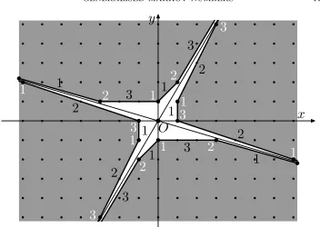
Figure 2. An arrangement, its sails, and the LLS sequences.
Definition 3.4. For a generic arrangement A denote by LLS(A) the LLS sequence ofA.
Example 3.5. In Figure 2 we consider an example of an arrangement in R2. We show four convex hulls for each of the cones in the comple-ment to this arrangecomple-ment with grey. The sails (i.e. the boundaries of these convex hulls) are endowed with integer lengths of the segments (black digits) and with integer sines of the integer angles (white digits). They form LLS sequences of two types:
• Two LLS sequences with a period (1,1,2,3): here integer lengths are 1 and 2, and integer sines are 1 and 3.
• Two LLS sequences with a period (3,2,1,1): here integer lengths are 1 and 3, and integer sines are 1 and 2.
In both cases the order is taken counterclockwise. Note that the integer sines of the first type of LLS sequences are the integer lengths of the second type LLS sequence and vise versa. This is an example of the classical duality between the LLS sequences of adjacent angles (see, e.g, in [23, Chapter 2]).
Remark 3.6. The techniques of sails goes back to the original works of F. Klein [26, 27] who used sails for the generalisation of classical continued fractions to the multidimensional sail. In fact the Klein multidimensional continued fraction seems to be an appropriate tool to study the multidimensional Markov spectrum. Further this method was explored in more detail by V. Arnold [3, 2] and his school (for more details see [23]). An alternative approach was proposed by J.H. Conway in [6]. Further K. Spalding and A.P. Veselov in [38] established a remarkable relation between Conway rivers and Klein-Arnold sails.
3.2. Generic reduced forms. Let us associate with every arrange-ment the following indefinite quadratic form.
Definition 3.7. We say that a form (y−px)(y−qx) isreduced if p >1 and 0> q >−1.
Denote it by fp,q.
We have a similar notion of generality for quadratic forms.
Definition 3.8. Letf be a quadratic form and letr be a real number. We say that f represents r if there exists some integer point (x, y) 6= (0,0) such that f(x, y) = r.
A quadratic form f is called generic if it does not represent 0. 3.3. Marked LLS sequences and reduced generic arrangements. Since the functionalMis zero at non-generic arrangements, it remains to study the properties of Mfor generic arrangements. Note also that Mis constant at every SL(2,Z)-orbit of integer generic arrangements. So it is enough to choose some representatives from all SL(2,Z)-orbits of integer generic arrangements.
Definition 3.9. We say that an integer generic arrangement formed by the lines y=pxand y =qx is reduced if
p >1 and 0> q >−1. Denote it by A(p, q).
In order to relate both-side infinite sequences to generic arrange-ments we need to fix a starting point of a sequence and a direction, so we need the following definition.
Definition 3.10. A both side infinite sequence of numbers is said to be marked if a starting element together with a direction are chosen.
Definition 3.11. Consider the LLS sequence of a reduced integer ar-rangement A = {y = px, y = qx} as above. Let A0 = (1,0) and
A1 = (1,⌊p⌋). We say that the LLS sequence with the starting point
a0 = lℓ(A0A1) and the direction induced by the orientation of the sail from A0 to A1 is the marked LLS sequence for the arrangement. We denote it by LLS∗(A).
Proposition 3.12. The map A → LLS∗(A) is a bijection between
the set of all generic reduced arrangements and the set of all marked
infinite sequences.
Let us formulate here a general proposition, relating slopes of the lines in the arrangement and the corresponding LLS sequence (for more details see [23, Chapter 3]).
Proposition 3.13. Consider the following two regular continued frac-tion expressions:
a+ = [a+0;a1 :. . .],
a− =−[a−0 :a−1 :a−2 :. . .]
where a±0 >0, and at least one of them is nonzero. Set also
a0 =a−0 +a+0. Then the LLS sequence of fa+,a− is (ai)
+∞
−∞, where a0 corresponds to the segment with endpoints (1, a−0) and (1, a+0).
For further details on arrangements and their LLS sequences we refer to the general theory of integer trigonometry [20, 21] and [23, Chap-ters 3,4].
3.4. Perron Identity in one diagram. The cornerstone of the the-ory of Markov Spectrum is the following classical theorem.
Theorem 3.14. Consider an indefinite binary quadratic form f with positive discriminant ∆(f). Assume that f does not attain zero at in-teger points distinct to the origin. Let A be the zero locus arrangement for f with
LLS(A) = (. . . a−2, a−1, a0, a1, a2. . . .) for some positive integers ai, i∈Z. Then
(1)
inf
Z2\{(0,0)} f
= inf
i∈Z
p
∆(f)
ai+ [0;ai+1 :ai+2 :. . .] + [0;ai−1 :ai−2 :. . .]
.
Marked infinite
sequences Generic reducedarrangements
Generic reduced quadratic forms
Elements of Markov spectrum
α
β
γ δ
ν
[image:14.612.163.448.114.251.2] [image:14.612.133.473.353.673.2]µ
Figure 3. Diagram for Perron Identity.
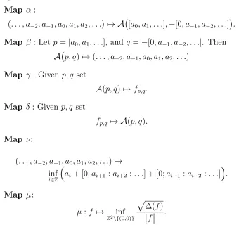
Let us rewrite the Perron Identity in the form of a diagram (See Figure 3). We will extend this diagram further to visualise Markov theory and to generalise it. Let us now describe the maps in this diagram.
Map α:
(. . . , a−2, a−1, a0, a1, a2, . . .)7→ A [a0, a1, . . .],−[0, a−1, a−2, . . .]
.
Map β : Let p= [a0, a1, . . .], and q=−[0, a−1, a−2, . . .]. Then
A p, q)7→(. . . , a−2, a−1, a0, a1, a2, . . .)
Map γ : Givenp, q set
A(p, q)7→fp,q.
Map δ: Given p, q set
fp,q 7→ A(p, q).
Map ν:
(. . . , a−2, a−1, a0, a1, a2, . . .)7→ inf
i∈Z
ai+ [0;ai+1 :ai+2 :. . .] + [0;ai−1 :ai−2 :. . .]
.
Map µ:
µ:f 7→ inf
Z2\{(0,0)} p
∆(f)
f
.
Remark 3.16. It is clear that α, β, γ, and δ are isomorphisms and in addition β = α−1 and δ = γ−1. These isomorphisms give natural identifications of the spaces of marked infinite sequences, the space of generic reduced arrangements, and the space of reduced quadratic forms. The maps ν and µ are described by the left hand side and the right hand side of Equation (1). The identifications provided by α, β, γ, and δ resulted in the Perron Identity.
Remark 3.17. Mapν (and, equivalently µ) does not have an inverse, as this map is not an injection. The sequences mapping to one value are shown in Examples 6.27 and 6.28 later.
Remark 3.18. Since all the maps corresponding to arrows with oppo-site directions of the diagram in Figure 3 are inverse to each other, the diagram is commutative. This leads to Theorem 3.14 on the Perron Identity.
4. Theory of Markov spectrum for integer forms
In this section we discuss Markov theory for indefinite forms with integer coefficients. We introduce reduced matrices and reduced forms and show their basic properties in Subsection 4.1. Further in Subsec-tion 4.2 we define extremal reduced forms for which Markov minima are precisely at (1,0); additionally we define extremal matrices and fi-nite sequences related to extremal forms. Finally in Subsection 4.3 we put together the most important relations of the theory of the Markov spectrum for integer forms in one commutative diagram.
4.1. Reduced matrices. In this subsection we introduce reduced ma-trices and reduced forms and show their multiplicative properties and relate them to the corresponding LLS sequences.
4.1.1. Definition of reduced associated matrices and associated forms.
We start with the following general definition.
Definition 4.1. Let (a1, . . . , an) be positive integers.
• The matrix
K2n−1 Kn 2
K1n−1 Kn 1
is said to be a reduced matrix associated to (a1, . . . , an), and denoted byMa1,...,an.
• The form Kn−1
1 x2+ (K1n−K2n−1)xy−K2ny2.
4.1.2. Basic properties of reduced matrices and reduced forms. Let us collect several important properties of reduced associated matrices and associated forms.
Proposition 4.2. Let (a1, . . . , an) and (b1, . . . , bm) be two sequences of positive integers. Then the following six statements hold.
(i) We have Ma1,...,an =
n
Q
i=1
Mai.
(ii) We have Ma1,...,an ·Mb1,...,bm =Ma1,...,an,b1,...,bm.
(iii) It holds detMa1,...,an = (−1)
n.
(iv) The eigenlines of Ma1,...,an are
y=αx and y=βx
where
α= [ha1;. . .:ani] and β =−[0;han :. . .:a1i].
Therefore the LLS sequence for the corresponding arrangement is pe-riodic with period (a1, . . . , an).
(v) The point (1,0) is a vertex of a sail for Ma1,...,an.
(vi) The form fa1,...,an annulates the eigenlines of Ma1,...,an.
Proof. Item (i). We prove the statement by induction on the number of elements n in the product.
Base of induction. The statement is tautological for n= 1.
Step of induction. Assume we prove the statement for all sequences of length n. Let us prove the statement for an arbitrary sequence α = (a1, . . . , an+1). First of all, from the definition of the continuant we get
K1n+1 =an+1K1n+K1n−1 and K2n+1 =an+1K2n+K2n−1.
Further we have
n+1
Y
i=1
Mai =Ma1,...,an ·Man+1 =
K2n−1 Kn 2
Kn−1
1 K1n
·
0 1 1 an+1
=
Kn
2 an+1K2n+K2n−1
Kn
1 an+1K1n+K1n−1
=
Kn
2 K2n+1
Kn
1 K1n+1
=Ma1,...,an+1.
Item (iv) This statement follows from general theory of SL(2,Z) re-duced matrices (Gauss Reduction theory) for the case of even n, see e.g. in [22] or in [23, Chapter 7]).
Consider now the case of a matrix Ma1,...,a2n+1. Notice that
M =Ma1,...,a2n+1,a1,...,a2n+1 = Ma1,...,a2n+1 2
.
Therefore, M has the same eigenlines asMa1,...,a2n+1. Now Item (iv) for
Ma1,...,a2n+1 follows directly from Item (iv) for M, which is true for M
by Gauss Reduction theory.
Item (v): Consider a triangle bounded by the eigenlines and the line y= 2x−2. On the one hand it contains the point (1,0). On the other hand the closure of its interior does not contain integer points other than (1,0) due to the explicit expression of Item (iv): for eigenlines.
Direct computation shows Item (vi). Remark 4.3. In this paper we use SL(2,Z)-reduced matrices which were used in so called Gauss Reduction theory (for more details see [25, 30, 29, 22] and also in [23, Section 7]). We should note that there is an alternative choice of matrices for which the main statements have a straightforward translation. The reduced matrices and alternative matrices are as follows:
K2n−1 Kn 2
K1n−1 Kn 1
and
Kn
1 K1n−1
Kn
2 K2n−1
.
Here one matrix is obtained from another by a swap of x and y coor-dinates.
It remains to mention here that the theory of these matrices follow Cohn matrices for the classical Markov case, where the corresponding tree is generated, for instance, by the following two Cohn matrices
M =
1 1 1 2
and N =
1 2 2 5
.
(In the notation of Subsection 5.5 below the corresponding triple-graph isGM,N(SL(2,Z),•).) Recall that Cohn matrices were introduced in [4, 5] by H. Cohn. They were used for the study of Markov numbers based on works [16] and [33].
Remark 4.4. It is interesting to note that any SL(2,Z) matrix
a c b d
that satisfies
Finite even sequences Extremal reduced SL(2,Z) matrices Extremal reduced
quadratic forms
Quadratic Markov spectrum
A B
C
D E
F
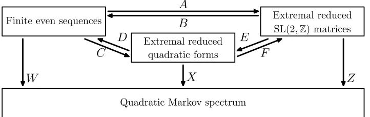
[image:18.612.127.488.123.237.2]W X Z
Figure 4. Sequences, forms, matrices, and Markov spectrum.
is reduced. It is then equivalent to the product of even number of matrices of elementary type Mai.
4.2. Extremal reduced forms, extremal reduced matrices, ex-tremal even sequences. We start with the following general remark. Remark 4.5. As we have seen from Proposition 4.2(iii) a matrix Ma1,...,an belongs to SL(2,Z) if and only if n is even. Further we
re-strict ourselves entirely to the case of SL(2,Z) matrices, and therefore we study the case of even finite sequences.
Let us finally give the following definition.
Definition 4.6.
• We say that a finite even sequence of integers is extremal if the associated form attains its normalised Markov minimum at point (1,0).
• An SL(2,Z) matrix associated to an extremal sequence is called
extremal.
• A form associated to an extremal sequence is calledextremal. 4.3. Theory of Markov spectrum for integer forms in one di-agram. In Figure 4 we show a diagram that gives bijections between the set of all finite sequences, extremal reduced matrices, and extremal reduced forms (Maps A-F). Additionally we have mappings to the Markov spectrum (Maps W, X, and Z). Let us describe these maps in more details.
Map A: Let (a1, . . . , an) be positive integers (here n is assumed to be even). Then
(2) (a1, . . . , an)7→Ma1,...,an =
Kn−1
2 K2n
K1n−1 Kn 1
Map B: For d > b > a ≥ 0 (and therefore c = adb−1) and the corresponding reduced matrix we have:
(3)
a c b d
7→Da1, . . . , a2n−1,
jd−1
b
kE
.
Here [a1;a2 : . . . : a2n−1] is the regular odd continued fraction decom-position for b/a.
Proposition 4.7. The maps A and B are inverse to each other.
In fact the map A can be extended analytically (i.e. with the same formula) to a bijection between the set of all finite sequences and the set of all reduced operators. This bijection delivers a complete invariant of SL(2,Z) conjugacy classes of SL(2,Z) matrices. A slightly modified version of this approach is known as Gauss Reduction theory (for more details see [29, 30, 25, 22] and [23, Chapter 7]).
Map C: For a finite sequence (a1, . . . , an) we set
(a1, . . . , an)7→fa1,...,an(x, y) =K
n−1
1 x2+ (K1n−K2n−1)xy−K2ny2.
Map D: We do not have a nice explicit form for this map. The map is a composition B ◦F. (See map F below).
Map E: We have the following simple formula here:
a c b d
7→bx2+ (d−a)xy −cy2.
Map F: Here we have
Ax2 +Bxy+Cy2 7→
a c b d
where
a= −B + √
B2−4AC+ 4
2 , b =A, c=−C, d=a+B.
Map W: For this map we have a nice expression in terms of contin-uants:
LLS7→
p
(Kn
1 +K2n−1)2−4
K1n−1
.
Map X: This is a restriction of Mapµ above. In addition we have the following useful formula:
f 7→
p
∆(f) f(1,0).
Map Z: This map is defined as follows:
a c b d 7→ p
(a+d)2−4
b .
Remark 4.8. Since all the maps corresponding to arrows with opposite directions of the diagram in Figure 4 are inverse to each other, the diagram is commutative, namely it holds for single elements, see for instance Figure 5 of Example 4.9.
Here and below to avoid ubiquity for a one element sequence (a) we write (a).
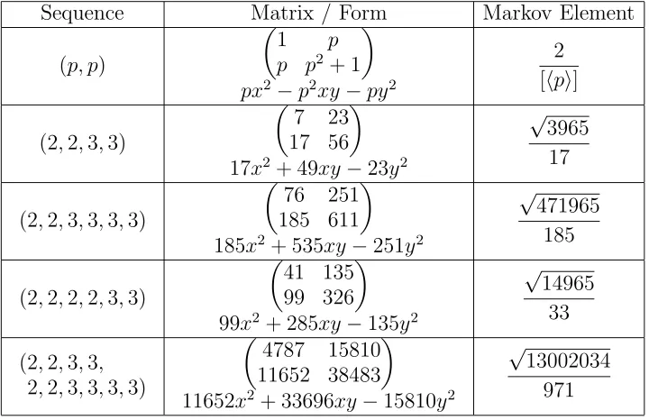
Example 4.9. Let us give several examples of various periods of LLS sequences together with corresponding matrices, forms, and Markov elements.
Sequence Matrix / Form Markov Element
(p, p)
1 p
p p2+ 1
px2 −p2xy −py2
2 [hpi]
(2,2,3,3)
7 23 17 56
17x2+ 49xy−23y2
√ 3965
17
(2,2,3,3,3,3)
76 251 185 611
185x2+ 535xy−251y2
√
471965 185
(2,2,2,2,3,3)
41 135 99 326
99x2+ 285xy−135y2
√ 14965
33
(2,2,3,3, 2,2,3,3,3,3)
4787 15810 11652 38483
11652x2+ 33696xy−15810y2
√
13002034 971
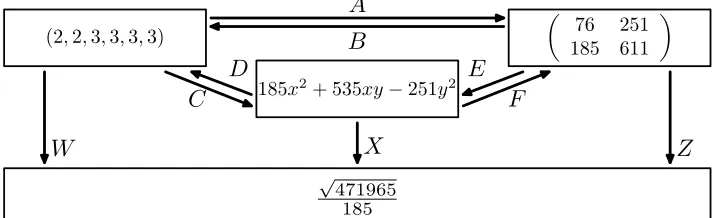
On the following diagram we consider a single case of the sequence (2,2,3,3,3,3) and its corresponding images under the above maps (see Figure 5).
[image:20.612.127.487.390.623.2](2,2,3,3,3,3)
76 251 185 611
185x2+ 535xy−251y2
√
471965 185
A B
C
D E
F
[image:21.612.127.485.125.234.2]W X Z
Figure 5. An example for (2,2,3,3,3,3).
Proposition 4.10. (i) After an appropriate SL(2,Z) change of coor-dinates any form corresponding to a periodic arrangement is multiple to some extremal reduced quadratic form.
(ii) Let A be an SL(2,Z) matrix. Then either A or−A is conjugate to some extremal form.
Proof. Item(i). Any form with a periodic arrangement determines the periodic LLS sequence α obtained by the compositions of Map δ and Map α of Figure 3. Take an even period of this LLS sequence and apply to it the map C. We get an extremal reduced quadratic form multiple to the original one.
Item (ii). The second statement is equivalent to Gauss Reduction theory in dimension 2 (see [23, Chapter 7]).
5. Triple-graphs: definitions and examples
5.1. Definition of triple-graphs. In this subsection we introduce a general triple-graph structure. Let S be an arbitrary set, and
σ :S3 →S
be a ternary operation on it, where S3 =S×S×S. Set
Lσ(a, b, c) = a, σ(a, b, c), b
, Rσ(a, b, c) = b, σ(b, c, a), c
.
Definition 5.1. Let S be an arbitrary set, and let σ be a ternary operation on it. Denote by G(S, σ) the directed graph whose vertices are elements of S3. The vertices v, w ∈ S3 are connected by an edge (v, w) if either
w=Lσ(v), or w=Rσ(v).
Definition 5.2. For a vertex v inG(S, σ) denote by Gv(S, σ) the con-nected component of G(S, σ) that contains v.
Definition 5.3. Any element w∈ Gv(S, σ) can be written as
(4) w=Ra2n
◦La2n−1
◦. . .◦Ra2
◦La1(v),
where a2, . . . , a2n−1 are positive integers and a1, a2n are nonnegative integers. We say that
(a1, a2, . . . , a2n)
is a Farey code of w inGv(S, σ), denote it by F(w). We say that the continued fraction
[0;a0+ 1 : a1 :. . .:a2n+ 1]
is a Farey coordinate of w, denote it by wF.
Definition 5.4. We say that a graphGv(S, σ) isfree generatedif every
w in Gv(S, σ) has a unique Farey coordinate (or in other words, the representation in Expression (4) is unique for every w inGv(S, σ)).
In case if Gv(S, σ) is free generated, the graph Gv(S, σ) is a binary rooted tree. Every element has a unique Farey code, and a unique Farey coordinate. Farey coordinates cover all rational numbers of the open interval (0,1).
5.2. Farey triples, Farey coordinates for triple-graph struc-ture. We start with a simple example of a triple-graph structure gen-erated by Farey triples. It is related to triangular chambers in Farey tessellation in hyperbolic geometry.
First of all we define Farey summation.
Definition 5.6. Let pq and r
s be two rational numbers with q, s > 0 and such that gcd(p, q) = gcd(r, s) = 1. Then
p q⊕ˆ
r s =
p+r q+s.
For a triple of rational numbers we set
ˆ
⊕(r1, r2, r3) =r1⊕ˆr2.
We have a triple-graphG(0/1,1/2,1)(Q,⊕ˆ). It turns out that this graph is free generated.
Proposition 5.7. Letvbe a triple ofG(0/1,1/2,1)(Q,⊕ˆ). Then its middle element coincides with its Farey coordinatevF.
In fact triples here are precisely the rational numbers in the vertices of triangles in Farey Tessellation (for further information we refer to [23, Section 23.2]).
5.3. Markov triple-graph. Consider the following ternary operation on the set of integers:
Σ(a, b, c) = 3ac−b.
We call this operation Markov multiplication of triples. By construction we have the following statement.
Theorem 5.8. The set of Markov triples coincides with the set of all triples obtained by permutation of elements in the vertices ofG(1,1,1)(Z,M).
Further we mostly consider a free generated part of it: G(1,5,2)(Z,Σ). Note that the complement to the set of vertices of G(1,1,1)(Z,M) for the set of vertices of G(1,5,2)(Z,M) is
(1,1,1),(1,2,1) .
5.4. Triple-graphs of finite sequences. LetZ∞ be the set of finite
sequences with integer elements. Consider a binary operation⊕onZ∞
defined as
(a1, . . . , an)⊕(b1, . . . bm) = (a1, . . . , an, b1, . . . bm).
Finally for a, b, c∈Z∞ set
⊕(a, b, c) =a⊕b.
Consider the triple-graph Z∞(a, b) = G(a,a⊕b,b)(Z∞,⊕). This graph is free generated if and only if a and b are not multiple to the same sequence c. Here we say that pis multiple toq if there exists an integer n such that
p=⊕ni=1q.
5.5. Triple-graphs of matrices. Let A, B, and C be SL(2,Z) ma-trices. Set
•(A, B, C) =AB. Now one can consider a triple-graph of matrices
G(A,AB,B)(SL(2,Z),•).
Definition 5.9. Let M and N be two SL(2,Z) matrices. Denote the triple graph G(M,M N,N)(SL(2,Z),•) by G•(M, N).
5.6. Tree structure of G⊕(µ, ν) and G• Mµ, Mν
. In this subsection we investigate when triple-graphs G⊕(µ, ν) andG• Mµ, Mν
has a tree structure.
5.6.1. A skew-lexicographical order. Let us introduce a standard order on the set of all finite and infinite sequences.
Definition 5.10. Let α = (pi)∞i=1 and β = (qi)∞i=1 be two infinite sequences of real numbers. We write α≻β if there exists n such that
pi =qi, i= 0, . . . , n−1;
pn > qn, if n is odd;
pn < qn, if n is even.
If α and β coincide, then we write α =β. In all the other cases we write α≺β.
Such ordering is called skew-lexicographic.
Recall that for a finite or infinite sequence of positive integers α = (a1, a2, . . .) we denote by [α] the following real number
From the general theory of regular continued fractions we have the following statement.
Proposition 5.11. Let µ and ν be two infinite sequences of positive integers. Then µ≻ν if and only if [µ]>[ν].
5.6.2. Evenly-composite sequences. In what follows we use the follow-ing general definition.
Definition 5.12. Let α be a finite even sequence. We say that α is
evenly-compositeif there exists an even sequence β such that α=β⊕β⊕. . .⊕β.
Otherwise we say that α is evenly-prime.
5.6.3. A skew-lexicographical order for concatenation of even sequences.
Now we prove a rather important proposition on skew-lexicographic order for concatenations.
Proposition 5.13. Letαandβ be evenly-prime sequences of integers. Assume that hαi ≺ hβi then we have
(i) hαi ≺ hα⊕βi ≺ hβi; (ii) hαi ≺ hβ⊕αi ≺ hβi.
Remark 5.14. Note that the skew lexicographic order for periodisa-tion of infinite sequences might be different from the skew-lexicographic order (naturally extended to finite sequences) for the sequences them-selves. For instance, in the case of α = (1,1,2,2,1,1) and β = (1,1,2,2), then β follows α, but hβi ≺ hαi.
Proof of Proposition 5.13. Item (i.2). First of all we prove that hα⊕ βi ≺ hβi.
The proof is split into the following three cases.
Case 1. Let β = αnαˆ, where n ≥ 1 and ˆα is an even sequence such that α= ˆα⊕α0 for some non-empty sequence α0.
By assumption we have
[hαi]<[hαnαˆi].
Hence by cancelling the first n copies of α (and since α consists of an even number of elements) we have:
[hαi]<[hααˆ ni].
Let us now compare the first several elements from both sides. We have
Here the middle inequality is equivalent to (since ˆα is even) [α0αˆ]≤[ ˆαα0].
Now if equality holds then α has a nontrivial even isomorphism, and therefore it is not evenly-prime. Hence we have a strict inequality:
[ααˆ]<[ ˆαα].
This implies that
[αn+1αˆ]<[αnααˆ ].
These are even partial fractions for [αβ] and [β] respectively. Hence [αβ]<[β].
We have completed the proof for Case 1.
Case 2. Now let β =αnαγˆ , where α <αγˆ , and difference is assumed at the very first element of γ. Here n ≥0, and ˆα is as in Case 1.
By assumption we have [hαi]<[hβi] and hence [hαi]<[hαnαγˆ i] Hence
[αβ] = [αn+1αγˆ ] = [αnααγˆ ]<[αnαγˆ ] = [β],
notice that here we manipulate finite continued fractions. The inequal-ity holds by the assumption.
The last inequality implies
[hαβi]<[hβi],
as this is true at the element with which γ starts inside β.
Case 3. Finally it remains to show the case β = ˆα 6= α (n = 0 of Case 1). We rewrite it as α=βmβˆ, where m >0 and ˆβ is a beginning of β with an even number of elements.
By assumption we have
[hαi] = [hβnβˆi]<[hβi].
Therefore, after cancelling βn at the beginning (since β has an even number of elements) we have
[hββˆ ni]<[hβi]. In particular
[ ˆββ]≤[ββˆ].
As in Case 1 (since β is evenly prime) the last inequality is strict. Therefore, we have
This concludes the proof for [hαβi]<[hβi].
Item(i.1).The casehαi ≺ hαβiafter cancelation of oneα is equivalent to
hαi ≺ hβαi. Let us rewrite it as
hβαi ≻ hαi.
Now the proof repeats the proof given above with all symbols ’<’ and ’≤’ changed to ’>’ and ’≥’ in all inequalities respectively.
Item (ii). Finally the proof for Item (ii) repeats the proof for Item (i) (for both statements) with all symbols ’<’ and ’≤’ changed to ’>’ and ’≥’ in all inequalities respectively and vice versa.
5.6.4. Skew-lexicographic order for G⊕(µ, ν). We start with the
follow-ing definition.
Definition 5.15. We say that a path v1, . . . , vn in a triple-graph G is descendingif for every i= 1, . . . , n−1 we have
vi+1 =Lσ(vi) or vi+1 =Rσ(vi).
Let α be a finite sequence. Recall that the periodisation hαi is a periodic infinite sequence with period α (see Definition 2.1).
Proposition 5.16. Letµandν be two evenly-prime sequences of inte-gers. Assume thathµi ≺ hνithen we have the periodisations of middle elements in the triple-graph G⊕(µ, ν) skew-lexicographically increasing
with respect to the Farey coordinate. Namely, let
(αi, βi, γi)∈ G⊕(µ, ν) for i= 1,2
with Farey coordinates wi
F for i= 1,2 respectively. Then
wF1 < wF2 implies hβ1i ≺ hβ2i.
Remark 5.17. Here we do not assume that the Farey coordinate is uniquely defined for the vertices of the triple-graph. We get the unique-ness of Farey coordinate later in Corollary 5.19.
Lemma 5.18. Let v1, . . . , vn be a descending path in a triple-graph
G⊕(µ, ν) with hµi ≺ hνi. Let alsovi = (αi, βi, γi) fori= 1, . . . , n. Then
hα1i ≺ hβni ≺(γ1).
Proof. Forn = 1 the statement follows directly from Proposition 5.13 and
By the induction on the number of operationsRandLand by Propo-sition 5.13 for every triple
(α, β, γ)∈ G⊕(µ, ν)
we have:
hαi ≺ hβi ≺ hγi.
The last directly implies the statement of Lemma 5.18.
Proof of Proposition 5.16. Let (αp, βp, γp) and (αq, βq, γq) be two triples of G⊕(µ, ν) whose Farey coordinates satisfy
(αp, βp, γp)F <(αq, βq, γq)F.
Consider the shortest path in the Farey tree connecting these two Farey coordinates. Let now the Farey coordinate of
(αc, βc, γc)∈ G⊕(µ, ν)
have the earliest tree level in this path.
Consider two descending paths in G⊕(µ, ν) that correspond to the
shortest paths in the tree from the c-triple to the p-triple and from the c-triple to the q-triple. Denote them by v1, . . . vn and w1, . . . wm respectively.
It is clear that v1 =w1 = (αc, βc, γc) , and that
v2 =L⊕(αc, βc, γc) and w2 =R⊕(αc, βc, γc).
Now on the one hand, by Lemma 5.18 applied to the pathv2, . . . , vn we have
hβpi ≺ hβci since βc is the third element in the triple v2.
On the other hand, by Lemma 5.18 applied to the path w2, . . . , wm we have
hβci ≺ hβqi since βc is the first element in the triplew2.
Therefore,
hβpi ≺ hβci ≺ hβqi.
Corollary 5.19. Let µ and ν be two evenly-prime sequences of in-tegers. Assume hµi ≺ hνi. Then the triple-graph G⊕(µ, ν) is a tree.
(In the other words, Farey coordinate is a complete invariant of
The last corollary can be reformulated for Generalised Gauss-Cohn matrices due to the fact that MapA has an inverse (see Equations (2) and (3)):
Corollary 5.20. Let µ and ν be two evenly-prime sequences of in-tegers. Assume hµi ≺ hνi. Then the triple-graph G•(Mµ, Mν) is a tree.
5.7. Reconstruction of triples in the triple-graphs by their cen-tral elements. The reconstruction of sequence triples in the triple-graphs by their central elements is based on the following simple propo-sition.
Proposition 5.21. Let µ and ν be two evenly-prime sequences of integers satisfyinghµi ≺ hνi. Suppose that a finite sequenceα /∈ {µ, ν} appears in some triple in the triple-graph G⊕(µ, ν). Then α appears
exactly once at the center of a triple.
Proof. Consider α /∈ {µ, ν}. Let α be an element of some triple in G⊕(µ, ν). Therefore α is constructed (i.e. appears at the highest
pos-sible level) as a concatenation of some other two sequences β and γ in some triple
(β, α, γ)∈ G⊕(µ, ν).
This implies the existence.
The uniqueness follows directly from Proposition 5.16.
Remark 5.22. Let us briefly mention that any triple of G⊕(µ, ν) is
reconstructible from its middle element.
From Proposition 5.21 we have a one-to-one correspondence between central elements and triples. So one can search the necessary triple by a brute force algorithm that studies all the triples level by level in the tree G⊕(µ, ν).
It remains to note that the middle LLS sequences in triples at leveln have at least 2nelements. Therefore the proposed brute force algorithm will stop in a time exponential with respect to the length of the central sequence.
Finite sequences inG⊕ (1,1),(2,2)
Extremal matrices in
G•(M(1,1), M(2,2))
Triples of reduced associated forms
Markov triples inG(1,5,2)(Z,M)
Discrete Markov spectrum
A B
C
D E
F P Q
R S T
W
Y Z
[image:30.612.127.485.110.313.2]X
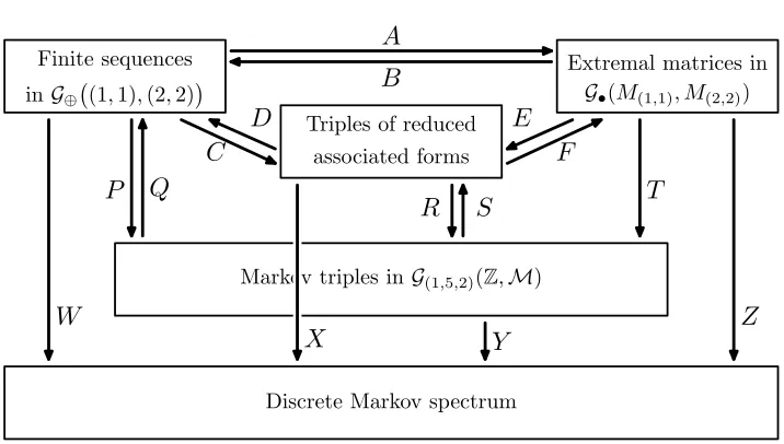
Figure 6. Classical Markov theory for extremal sequences.
6. Markov tree and its generalisations
In this section we discuss a generalisation of the Markov tree. First of all we reformulate a classical theorem in our settings and write the diagram for it in Subsection 6.1. Further we define Markov LLS triple-graphs in 6.2 and extend the definition of Markov triples in Subsec-tion 6.3. The properties of this generalisaSubsec-tion are collected in the di-agram of Subsection 6.4 (see Theorem 6.20). In Subsection 6.5 we recall the Uniqueness conjecture for Markov triples. Finally in Subsec-tion 6.6 we show counterexamples to the generalised Markov conjecture (see Examples 6.27 and 6.28).
6.1. Classical Markov theory in one diagram. On the diagram in Figure 6 we show all the maps that arise in classical Markov theory for the discrete Markov spectrum. Further in Section 6.4 we generalise this diagram to the cases of triple-graphs with different LLS sequences.
In fact Map C here is a definition of triples of associated forms:
Definition 6.1. MapC of Figure 6 is induced by the map which was considered in the periodic case above (see Figure 4):
(a1, . . . , an)7→fa1,...,an(x, y) =K
n−1
1 x2+ (K1n−K2n−1)xy−K2ny2.
We say that the (ordered) triples of forms obtained by such map are
Remark 6.2. These forms are simply related to the forms studied by A. Markov. After the following integer lattice preserving coordinate transformation:
x y
7→
−x−2y y
the associated forms from the above definition are taken to the forms of Theorem 1.5 by A. Markov. (In fact, this transformation corresponds to a one element shift in the LLS sequence.)
Remark 6.3. Maps A–F,W,X,Z considered coordinatewise are ac-tually restrictions of the corresponding maps in the diagram of Figure 4 in previous section. So we skip their description here.
Remark 6.4. The central form in the associated triple forms uniquely determines the central LLS sequence (via the compositionB◦F). The other two forms of the triple are uniquely reconstructed by the brute force reconstruction of associated forms from reduced forms via build-ing the tree of LLS sequences, as in Remark 5.22.
Map P: Consider a triple
(α, β, γ)∈ G⊕ (1,1),(2,2)
.
then we set
(α, β, γ)7→ K˘(α),K˘(β),K˘(γ)
.
Map Q: This map is extracted from the Theorem 1.5 by A.Markov. Consider a triple (a, M, b) whereM > b > a. Letube the least positive integer satisfying either of the following two equations
(5) ±ua ≡b mod M.
Let
M
u = [a1, . . . , a2n−1]
be the odd regular continued fraction for M/u. (Note that it is impor-tant to take the odd continued fraction here.) Then the period of the marked period for the corresponding LLS sequence is
(a, M, b)7→(a2n−1, . . . , a1,2).
Map R:
(f1, f2, f3)7→
f1(1,0), f2(1,0), f3(1,0)
Map S: Consider a triple (a, M, b) where we reorder the elements in the following way: M > b > a. As in Map Q let u be defined by Equation (5). Set
v = u 2+ 1
M .
Then Map S at the triple (a, M, b) is defined as
(a, M, b)7→Mx2 + (M+2u)xy+ (u+v−2M)y2.
Remark 6.5. Here the pair (u, v) is defined as in Markov’s theorem (Theorem 1.5), with an obvious change of coordinates inverse to the one introduced in Remark 6.2.
Remark 6.6. Note that u and v are defined by the triple (a, M, b). The statement that u and v may be reconstructed entirely by M is equivalent to the uniqueness conjecture.
Map T: Here we have a coordinate mapping between a triple of matrices and a Markov triple
a b c d
7→c.
Map Y: This map is provided by Markov’s theorem (Theorem 1.5).
(a, M, b)7→ √
9M2−4
M .
The existence of the inverse to Map Y is equivalent to the uniqueness conjecture (see Remark 6.26).
Remark 6.7. Since all the maps corresponding to arrows with opposite directions of the diagram in Figure 6 are inverse to each other, the diagram is commutative. This gives a core for the classical Markov theory.
6.2. Markov LLS triple-graphs. Let us describe almost Markov and Markov LLS triple-graphs.
For real a, bwe set
ga,b= (x−ay)(x−by).
Denote by U+,+a,b the region defined by x−ay >0 and x−by >0.
Definition 6.8. Letµandνbe two evenly-prime sequences of integers. Let the following be true:
• the global minima of g[hµi],−[0;hµi] at nonzero integer points of the cone U+,+[hµi],−[0;hµi] is attained at (1,0).
• the global minima ofg[hνi],−[0;hνi]at nonzero integer points of the cone U+,+[hνi],−[0;hνi] is attained at (1,0).
Then the triple-graph G⊕(µ, ν) is called the almost Markov LLS triple-graph.
Definition 6.9. We say that an even finite sequenceα = (a1, . . . a2n) is evenly palindromicif there exist an integerk such that for every integer m we have
ak+m mod 2n =ak−m−1 mod 2n.
Definition 6.10. An almost Markov LLS triple-graph G⊕(µ, ν) is a Markov LLS triple-graphif
• every sequence in every triple ofG⊕(µ, ν) is evenly palindromic.
Example 6.11. Let m, n≥1 and p > q ≥1. Then for the sequences µ= (p)2n
, ν = (q)2m
the first three conditions are straightforward, and the palindrome con-dition is proved in [40]. Note that the case p= 1, q = 2, m = n = 1 corresponds to the classical case of Markov tree G⊕ (1,1),(2,2)
.
Example 6.12. Let m, n ≥ 1 and p > q ≥ 1, and α be an evenly palindromic sequence. Then
µ= (p)2n
, ν = (p)2mα
satisfies the fourth condition. Here one can construct many examples satisfying the first three conditions. For instance, one can take
µ= (5,5,1,2,2,1) and ν = (5,5).
Problem 1. Describe all pairs of sequences µ, ν for which the triple-graph G⊕(µ, ν) is Markov/almost Markov.
Remark 6.13. A very important property for a Markov triple-graph G⊕(µ, ν) is as follows. For every element of every triple the
corre-sponding reduced form has a normalised Markov minimum at (1,0) (see Corollary 7.11). This property allow us to relate LLS sequences and corresponding matrices directly with elements of the Markov spec-trum.
Remark 6.14. For an almost Markov graphG⊕(µ, ν) we have a slightly
(4,191,11) (191,23489,11)
(4,3427,191)
(23489,2888956,11)
(191,50806696,23489)
(3427,7412597,191)
(4,61495,3427)
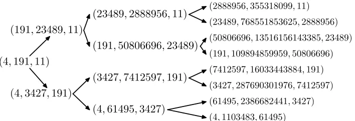
[image:34.612.131.485.115.236.2](2888956,355318099,11) (23489,768551853625,2888956) (50806696,13516156143385,23489) (191,109894859959,50806696) (7412597,16033443884,191) (3427,287690301976,7412597) (61495,2386682441,3427) (4,1103483,61495)
Figure 7. The first 4 levels in the tree T(4,4),(11,11).
Remark 6.15. Note that there is a nice expression for Map W in the case of G⊕((1,1),(2,2)). Here for every sequence (a1, . . . , an) in every triple of G⊕((1,1),(2,2)) have
W(a1, . . . , an) =an+ [0;ha1, . . . , ani] + [0;han−1, . . . , a1, ani].
6.3. Generalised Markov and almost Markov triples. Starting from Markov/almost Markov LLS triple-graphs one can define gener-alised Markov/almost Markov graphs. In this subsection we discuss the triple-graph structure for them.
6.3.1. Generalised Markov/almost Markov graphs.
Definition 6.16. Consider a Markov/almost Markov LLS triple-graph G⊕(µ, ν) and replace each triple of sequences (α, β, γ) by a triple of
integers K˘(α),K˘(β),K˘(γ)
. The resulting triple-graph is called the
generalised Markov/almost Markov graph and denoted by Tµ,ν.
The triples of generalised Markov/almost Markov graph are called
generalised Markov/almost Markov triples.
Example 6.17. In Figure 7 we show the first four layers of the ex-tended Markov triple-graph T(4,4),(11,11). By construction we automat-ically have: v2 > v1, v3. Note that we do not require v2 > v3 > v1 as it was for the Markov tree, so if a similar order is needed one should swap v1 and v3 if necessary.
6.3.2. Triple-graph structure for generalised Markov and almost Markov graphs. In order to define the triple-graph structure on Tµ,ν we should extend the operation
Σ : (a, b, c) = 3ac−b
The main difficulty here is that a straightforward operation on the graph Tµ,ν is defined by sequences rather then by triples:
(6) Σ˜(α, a),(β, b),(γ, c)= ˘K(α⊕β),
where (α, β, γ)∈ G⊕(µ, ν) is the triple defining (a, b, c).
Here one should remember all the sequences together with triples, combining togetherTµ,ν andG⊕(µ, ν). Hence we arrive to the following
ternary operation on the product Z∞×Z:
⊗(α, a),(β, b),(γ, c)=α⊕β,Σ (˜ α, a),(β, b),(γ, c)
.
Now we can give the following definition.
Definition 6.18. Denote by G⊗(µ, ν) the triple-graph
G(µ,K(µ)),(µ˘ ⊕ν,K(µ˘ ⊕ν)),(ν,K(ν))˘ (Z∞×Z,⊗). In fact as we show in Corollary 7.19, we have
(7) Σ˜(α, a),(β, b),(γ, c)= K˘(α⊕α) ˘
K(α) b−c.
Remark 6.19. In the classical case of G⊗ (1,1),(2,2)
we have
˘
K(α⊕α) ˘
K(α) = 3a
(see Proposition 7.21 later) and hence
˜
Σ(α, a),(β, b),(γ, c)= Σ(a, b, c) = 3ac−b.
This establishes a straightforward equivalence between the triples of T(1,1),(2,2) and the triples of G⊗ (1,1),(2,2)
.
So there is a natural question here.
Problem 2. For which triple-graphsG⊗(µ, ν) is the function ˜Σ a
func-tion on triples (a, b, c) (and not depend on α)?
This is equivalent to the following one.
Problem 3. For which pairs of even sequences (µ, ν) does every triple of Tµ,ν occur only once in the tree.
Finite sequences in
G⊕ µ, ν
Extremal matrices in
G•(Mµ, Mν)
Reduced quadratic forms
Generalized Markov triples inG⊗(µ, ν) (or inTµ,ν)
Discrete Markov spectrum
A B
C
D E
F P Q
R S T
W
Y Z
[image:36.612.126.485.114.313.2]X
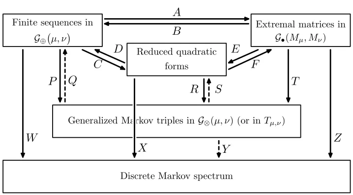
Figure 8. Extended Markov theory for extremal sequences.
6.4. Generalised Markov theory in one diagram. Finally for gen-eralised Markov triple-graphs we have the following diagram.
Let G⊗(µ, ν) be a graph for some generalised Markov
triple-graph Tµ,ν. The extension of classical Markov theory for this triple-graph is presented in the diagram of Figure 8. As we will discuss later in Subsection 7.3, some triple-graphs G⊗(µ, ν) can be reconstructed
from the triple-graph Tµ,ν.
In the diagram of Figure 8 most of the maps are literally exten-sions from the classical case of Figure 6. This follows directly from Corollary 7.11 (which we show below). All of the forms corresponding to generalised Markov triple-graphs have a normalised Markov mini-mum at (1,0), and therefore by Definition 4.6 they are extremal. This observation leads to the fact that the properties that A. Markov has detected on a particular example of discrete Markov spectrum could be seen much wider. As a consequence we have the following theorem.
Theorem 6.20. Let G⊗(µ, ν) be a triple graph for some generalised Markov triple-graphTµ,ν Then the maps of the diagram of Figure 8 are defined as follows.
• The maps
A–F, W, X, Z
• The maps P, R and S are as in Figure 6:
P : (α, β, γ)7→ K˘(α),K˘(β),K˘(γ)
; R : (f1, f2, f3)7→
f1(1,0), f2(1,0), f3(1,0)
;
T :
ai bi
ci di
i= 1,2,3
7→(c1, c2, c3).
• Finally: MapQ is trivial; while MapsS andY are derived from mapsC and W respectively for the triple-graph G⊗(µ, ν).
This theorem confirms that a remarkable structure discovered by Markov for the discrete Markov spectrum has a general nature in ge-ometry of numbers.
Let us finalise this section with several important remarks concerning the diagram of Figure 8.
Remark 6.21. Explicit expressions for MapsQ, S, and Y for Tµ,ν (in case of existence) are not known to the authors. For this reason they are marked by dashed lines.
Remark 6.22. Similar to the Markov settings, all the triples in the Generalised Markov diagram are reconstructible by the middle element in a unique way (see Remark 5.22 and Remark 6.4).
Remark 6.23. Corollary 7.11 below is crucial for the mapsW,X, and Z of this section. It establishes a connection between sequences, forms, and matrices on the one hand and the elements of Markov spectrum on the other hand.
Remark 6.24. Similar to the classical Markov case (see Figure 6) the maps corresponding to arrows with opposite directions in the diagram in Figure 8 are inverse to each other. Therefore the diagram in Figure 8 is commutative.
6.5. Uniqueness conjecture for Markov triples. The following conjecture is due to G. Frobenius.
Conjecture 4. (Uniqueness conjecture, 1913.) Every Markov number appears exactly once as the maximum in a Markov triple.
Remark 6.25. The uniqueness conjecture is a slightly modified version of the fact that X is one-to-one with its image.
Remark 6.26. If we restrict Y from Markov triples to single Markov numbers, then we have one-to-one map with an image established by
M 7→ √
9M2−4
M
(which is an increasing function of positive numbers).
So it is not known if it is possible reconstruct M 7→ (a, M, b). As we show in Examples 6.27 and 6.28, this is not always the case for generalised Markov numbers.
6.6. A counterexample to the generalised uniqueness conjec-ture. First of all we formulate the uniqueness conjecture for gener-alised Markov numbers.
Conjecture 5. (Generalised uniqueness conjecture, 2018.) Con-sider a generalised Markov triple-graphTµ,ν. Every generalised Markov number appears exactly once as a maximal (middle) element in a Markov triple in Tµ,ν.
Studying the extended Markov numbers of T(p,p),(q,q) for different (p, q) we have spotted two counterexamples to the generalised unique-ness conjecture. They are both for p= 4 and q = 11. (Note that the first layers of the corresponding triple-graph are shown in Figure 7.)
Example 6.27. First of all consider
α1 = 4,4,(11)8 α2 = (4)12,11,11 We have
˘
K(α1) = ˘K(α2) = 355318099,
and hence Map Y is not injective. This implies that the associated forms
355318099x2+ 3856825285xy−928389367y2 and
355318099x2+ 3856242857xy−930136651y2
have the same normalised Markov minima. Therefore the number 355318099 appears at least twice as a maximal (middle) element in the generalised Markov triples of the triple-graph G⊕ (4,4),(11,11)
Example 6.28. The second example is for α1 = 4,4,(11)14
α2 = (4)22,11,11
. Here
˘
K(α1) = ˘K(α2) = 661068612553111.
The corresponding forms are respectively
661068612553111x2+ 7175615729089857xy−1727266560524267y2 and
661068612553111x2+ 7174532122960713xy−1730517378911699y2.
Remark 6.29. The arrangements of zero lines for the forms of Exam-ples 6.27 and 6.28 are not integer congruent to each other, since they have different LLS sequences.
7. Related theorems and proofs
In this section we prove several theorems that are used in generalised Markov theory. In Subsection 7.1 we prove that any Markov LLS triple-graph G⊕(µ, ν) has Markov minima at (1,0) and that these minima
are unique up to the integer symmetries of the sail containing (1,0). Further in Subsection 7.2 we prove that the triples of the triple-graph G⊗(µ, ν) satisfy Equation (7) on page 35. Finally in Subsection 7.3 we
prove the first results towards a solution of Problem 2.
7.1. Concatenation of sequences and global minima of the cor-responding forms. In this section we formulate and prove one of the central results of the current paper (Corollary 7.11), which states that all the forms have a normalised Markov minimum (see Definition 1.1). This result is crucial for linking extended Markov numbers with nor-malised Markov minima for them.
Recall that for real a, bwe consider
ga,b= (x−ay)(x−by),
and thatU+,+a,b denotes the region defined byx−ay > 0 andx−by >0.
Lemma 7.1. Let a and b be two real numbers. Consider a point v = (x, y) of the region U+,+a,b , and let ε be a positive real number. Then the following hold.
(i) If y >0 then
ga+ε,b(v)< ga,b(v)
ga,b+ε(v)< ga,b(v) .
(ii) If y <0 then
ga+ε,b(v)> ga,b(v)
ga,b+ε(v)> ga,b(v) . (iii) If y= 0 then
ga±ε,b(v) = ga,b(v)