Fire at high latitudes: Data-model comparisons and their consequences

consequences

.

White Rose Research Online URL for this paper:

http://eprints.whiterose.ac.uk/86266/

Version: Published Version

Article:

Kantzas, E., Lomas, M. and Quegan, S. (2013) Fire at high latitudes: Data-model

comparisons and their consequences. Global Biogeochemical Cycles, 27 (3). 677 - 691.

ISSN 0886-6236

https://doi.org/10.1002/gbc.20059

[email protected] https://eprints.whiterose.ac.uk/ Reuse

Unless indicated otherwise, fulltext items are protected by copyright with all rights reserved. The copyright exception in section 29 of the Copyright, Designs and Patents Act 1988 allows the making of a single copy solely for the purpose of non-commercial research or private study within the limits of fair dealing. The publisher or other rights-holder may allow further reproduction and re-use of this version - refer to the White Rose Research Online record for this item. Where records identify the publisher as the copyright holder, users can verify any specific terms of use on the publisher’s website.

Takedown

If you consider content in White Rose Research Online to be in breach of UK law, please notify us by

Fire at high latitudes: Data-model comparisons

and their consequences

Euripides Kantzas,1Mark Lomas,2and Shaun Quegan1

Received 12 June 2012; revised 8 May 2013; accepted 21 June 2013; published 9 August 2013.

[1] Fire is an endemic process at high latitudes, connected to a range of other land surface

properties, such as land cover, biomass, and permafrost, and intimately linked to the carbon balance of the high-latitude land surface. Much of our current understanding of these links and their climate consequences is through land surface models, so it is important to ensure that for their credibility, these models should be consistent with available data. Over the vast panboreal region, a key source of information onfire is satellite data. Comparisons between satellite-based burned area data from the Global Fire Emissions Database and three dynamic vegetation models (LPJ-WM, CLM4CN, and SDGVM) indicate that all models fail to represent the observed spatial and temporal properties of thefire regime. Although the three dynamic vegetation models give comparable values of the boreal net biome production (NBP),fire emissions are found to differ by a factor 4 between the models, because of widely different estimates of burned area and because of different parameterizations of the fuel load and combustion process. Including a more realistic representation of thefire regime in the models shows that for northern high latitudes, (i) severefire years do not coincide with source years or vice versa, (ii) the interannual variability offire emissions does not significantly affect the interannual variability of NBP, and (iii) overall biomass values alter only slightly, but the spatial distribution of biomass exhibits changes. We also demonstrate that it is crucial to alter the current representations offire occurrence and severity in land surface models if the links between permafrost andfire are to be captured, in particular, the dynamics of permafrost properties, such as active layer depth. This is especially important if models are to be used to predict the effects of a changing climate, because of the consequences of permafrost changes for greenhouse gas emissions, hydrology, and land cover.

Citation: _{Kantzas, E., M. Lomas, and S. Quegan (2013), Fire at high latitudes: Data-model comparisons and their}

consequences,Global Biogeochem. Cycles,27, 677–691, doi:10.1002/gbc.20059.

1. Introduction

[2] Land masses at northern high latitudes, defined in this

paper as poleward of 50°N and including the boreal and Arctic land masses, are characterized by huge expanses of boreal forest, wetlands, peatlands, and tundra lying on or-ganic soils that account for 50% of the global belowground organic carbon [Tarnocai et al., 2009]; northern peatlands alone hold a third of the global soil organic matter [Turetsky et al., 2002]. Large parts are underlain by perma-frost (continuous, widespread, or scattered). Low-average annual air temperatures have caused the rate of carbon

deposition to be on average higher than decomposition through the Holocene Era, leading to net accumulation of carbon; over-all, these regions hold a third of the global terrestrial carbon [McGuire et al., 1995]. Atmospheric inversion studies show that the high-latitude land surface continues to act as a carbon sink, estimated as 0.23 ± 1.22 Pg C yr 1 _{by Gurney et al.} [2003], 0.19 ± 0.53 Pg C yr 1 by Baker et al. [2006], and 0.38 ± 0.27 Pg C yr 1_{byRödenbeck et al. [2003].}

[3] Projections of the temperature response to climate

show considerable warming of northern latitudes in the 21st century [Christensen et al., 2007; Serreze and Francis, 2006]. Since 1900, the temperature in the Arctic has in-creased by 0.09°C per decade [Corell, 2005] and is projected to increase by 0.25–0.75°C per decade over the next 100 years, with associated increases in precipitation [Christensen et al., 2007]. However, the effects of increased temperature on physical processes in the Arctic, the sensitiv-ity of the carbon cycle to such changes, and the size of climate-carbon cycle feedbacks in this region remain highly uncertain [Friedlingstein et al., 2006; McGuire et al., 2009]. Such processes include the following: (a) decrease of snow cover and its effect on albedo and the radiation 1

Centre for Terrestrial Carbon Dynamics: National Centre for Earth Observation, University of Sheffield, Sheffield, UK.

2

Department of Animal and Plant Sciences, University of Sheffield, Sheffield, UK.

Corresponding author: E. Kantzas, Centre for Terrestrial Carbon Dynamics: National Centre for Earth Observation, University of Sheffield, Hicks Bldg., Hounsfield Rd., Sheffield S37RH, UK. (e.kantzas@sheffield.ac.uk)

budget; (b) changes in thefire regime, withfire-resistant spe-cies benefiting from increased disturbance; (c) permafrost thawing and water table changes in peatlands with subse-quent release of carbon and methane; and (d) increased photosynthesis with shrub and tree establishment at higher latitudes. For example, even though global circulation models driven by emissions scenarios show an increase in fire activity in boreal forests [Stocks et al., 1998], analysis of the last 15 years of activefire data shows no statistically significant increase [Arino et al., 2012]; however, the period examined is substantially smaller than thefire return interval at boreal latitudes, which usually exceeds 100 years [Kasischke et al., 1995], so it does not allow a safe conclu-sion regarding trends.

[4] As pointed out byCox and Stephenson[2007], during

thefirst 10 years of a climate projection, the anthropogenic climate change signal is small compared to the decadal vari-ability of climate, so over this period, the uncertainties in the projection originate mostly from the initial conditions used to describe the system, whereas at later times, they originate from errors in model formulation and uncertainties in the emission scenarios. A significant amount of work has been undertaken in recent years to address the initial value prob-lem and to improve parameterizations by establishing a set of Essential Climate Variable data sets under the framework established by the Global Climate Observing System [GCOS, 2004, 2010]. This study focuses on fire-related Essential Climate Variables and processes at latitudes pole-ward of 50°N. To allow compact terminology, we will refer to this region as the boreal zone, even though it contains, for example, some temperate zones under maritime infl u-ence. In this region,fires provide a means to transfer large quantities of terrestrial carbon into the atmosphere with high spatial and temporal variability. Several studies using climate projections have hinted at a potential increase in burned area and length of thefire season in the boreal region [Flannigan and Vanwagner, 1991;Wotton and Flannigan, 1993] with an associated loss in stored carbon [Kasischke et al., 1995], while on a global scale, increasing temperatures could act as a driver of the fire regime, leading to positive carbon feedbacks [Pechony and Shindell, 2010]. Nevertheless,fire dynamics are thought to be poorly represented in global climate models [Bowman et al., 2009], as this paper clearly confirms for high northern latitudes. Marked differences are found between the properties of fires observed by sat-ellites and their representations in three state-of-the-art land surface models, two of which are embedded in Intergovernmental Panel on Climate Change standard cli-mate models. This raises important questions about the models and their ability to provide meaningful predictions under a changing climate:

[5] 1. Does the models_’failure to capture the

spatiotem-poral variability in fire matter when estimating the effects of fire on high-latitude processes and quantities, such as net biome production (NBP), biomass, and the dynamics of permafrost?

[6] 2. Are there empirical data on the sizes of the carbon

pools available as fuel in the boreal zone and their combus-tion completeness, and can these be used to test the models? [7] 3. Can the models be reparameterized to conform better

with observational data, and what are the consequences? [8] These are addressed in the latter part of the paper.

2. Models, Data, and Methods

2.1. Description of Models

[9] Three dynamic vegetation models (DVMs) are used in

this study, of which two, the Lund-Potsdam-Jena (LPJ) dy-namic global vegetation model [Sitch et al., 2003] and the Community Land Model 4 (CLM4) [Kloster et al., 2010], are embedded in coupled climate models (the Bergen Climate Model [Tjiputra et al., 2010] and the Norwegian Earth System Model, respectively). The third, the Sheffield Dynamic Global Vegetation Model (SDGVM), is a stand-alone terrestrial carbon-water model, chosen because of the ease with which it can be modified and used to test hypothe-ses within this study. Brief descriptions of these models are given below, focusing mainly on their relevance to studying carbon- andfire-related processes at high latitudes. Fuller de-scriptions are available in the references, and a detailed com-parison of process representations in LPJ and SDGVM is given inQuegan et al. [2011].

[10] LPJ-WM [Wania et al., 2009] is an enhanced version

of LPJ tailored to high-latitude biomes, with adaptations to model peatland vegetation, peatland hydrology, and perma-frost dynamics. It includes two new plant functional types (PFTs),flood-tolerant C3 graminoids and mosses: the latter represents the class of bryophytes, which have significant ef-fects on the Arctic carbon balance [Street et al., 2012]. For peatland hydrology, a new parameterization was introduced which considers the specific dynamics found in peat soils. To estimate permafrost behavior and permafrost active layer depth, soil temperature is calculated as a function of depth by numerically solving the one-dimensional heat diffusion equation using the Crank-Nicolsonfinite difference scheme in a column which incorporates snow, litter, and 12 soil layers, with an upper boundary condition given by the air temperature and a lower boundary condition of stable tem-perature. This required the hydrology module [Gerten et al., 2004] to be modified to permit a greater number of soil layers.

[11] CLM4CN [Lawrence et al., 2011] is an updated

ver-sion of CLM4, the land component of the Community Earth System Model [Collins et al., 2006], with a prognostic carbon-nitrogen biochemical model. CLM4CN has specific parameterizations for the thermal and hydraulic properties of organic soil [Lawrence and Slater, 2008] and incorporates boreal PFTs, and its soil temperature profiles and permafrost extent perform well when compared to observations [Lawrence et al., 2008].

[12] The SDGVM [Woodward and Lomas, 2004;Woodward

et al., 1995] is one of the earliest of a host of DVMs which are now available. It has been used in several DVM comparison studies [Cramer et al., 2001;Le Quere et al., 2009; Piao et al., 2009] and has proven to be a good indicator of the gen-eral trends produced by DVMs at global and regional scales. It contains no specific adaptations to high latitude conditions, e.g., it does not contain a permafrost module but is well suited to investigating the effects of land cover and some aspects offire.

2.1.1. Fire Representation in Models

[13] Comparison of the three models is aided by the fact

temperature and moisture. It is then weighted against the available fuel in the grid cell, and finally, according to a model-specific set of rules that govern the combustion pro-cess, thefire emissions are calculated. A crucial observable quantity is therefore the burned area, which is derived in dif-ferent ways between the models.

[14] In LPJ-WM, the probability offire for a grid cell is

cal-culated daily as a function of litter moisture, with temperature and available litter acting as limiting factors [Thonicke et al., 2001]. By summing the daily probability over the course of the year, the annual length of the fire season is calculated, from which the annual fraction burned in each grid cell is es-timated and distributed across the PFTs in proportion to the area they cover. CLM4CN incorporates the LPJ-WM algo-rithm to estimate the burned area [Kloster et al., 2010] with modifications by Thornton et al. [2007] to accommodate the subdaily time step used by CLM and to adapt to the spe-cifics of its variables, not all of which have exact equivalents in LPJ-WM. SDGVM produces burned area by an empirical model driven by monthly averages of temperature and precipitation and limits thefire return interval (FRI) to lie be-tween 2 and 800 years, which in land surface process models is defined as the time required for successivefire events to cu-mulatively burn an area equal to the area of interest, usually a grid cell of a given spatial resolution. Hence, the FRI is equal to the reciprocal of the annual average fraction of area burned. None of the models incorporates fire propagation mechanisms within a grid cell or between neighboring grid cells; instead, as in most land surface models at such resolu-tion, no lateralfluxes are included.

2.2. Fire and Climate Data

2.2.1. Satellite-Based Fire Products

[15] Three types of fire products are obtained from Earth

Observation (EO) data: activefires, burned area, andfire radia-tive power. Acradia-tive fire products, such as the Along Track Scanning Radiometer World Fire Atlas [Arino et al., 2012] and the Moderate Resolution Imaging Spectroradiometer (MODIS) MOD/MYD14CMH product [Giglio, 2010], use the thermal channels of sensors to register anomalies of the surface temperature and thus identify hot spots. Burned area products, like the MODIS MCD45A1 (MODIS-BA) [Roy et al., 2008] and the Global Fire Emissions Database-Burned Area (GFED-BA) [Giglio et al., 2010], are derived by identify-ing reflectance changes in the visible channels of the sensor; GFED-BA also makes use of activefire products in its retrieval algorithm. Finally, Fire Radiative Power, as in the MODIS product MOD/MYD14CMH, is obtained from the thermal channels of a sensor and is a measure of the rate of radiant heat, which is related to the rate at which fuel is consumed [Wooster et al., 2005].

[16] Both MODIS-BA and GFED-BA are examined in this

study. MODIS-BA uses images acquired from the MODIS satellite series and calculates the date of burn for each 500 m pixel, from which burned area can be retrieved. Data are available for the years 2000–2011 but only for latitudes below 70°N. GFED-BA merges several types of EO data and products, of which the majority come from MODIS im-ages, to create a global burned area data set at 0.5° resolution for the years 1996–2010; this is the same resolution as is used in all the models in this study.

[17] The GFED data set also contains estimates of carbon

dioxide and other trace gas emissions fromfire derived by a combination of satellite observations and modeling. Net pri-mary production isfirst calculated from estimates of the frac-tion of available photosynthetically active radiafrac-tion derived from EO data and allocated to plant types according to pre-scribed land cover. The Carnegie-Ames-Stanford Approach (CASA) biochemical model [Potter et al., 1993] is then used to calculate the carbon pools (biomass, litter, etc.) in each 0.5° grid cell. Using the GFED burned area product, emis-sions for each carbon pool are then calculated as a function of monthly burned area, mortality, and combustion com-pleteness, the last of which is calculated as a linear function of soil moisture. On a continental scale, the greatest uncer-tainties in carbon emissions are found in the boreal regions [van der Werf et al., 2010].

[18] Although activefire products cannot be directly used

in assessing model performance, they are important as they contribute to the GFED-BA burned area product. Fire Radiative Power has great potential for constraining models since it provides direct estimates of emissions from biomass burning [Roberts and Wooster, 2008], but no consistent data set for the boreal region yet exists, and hence, it is not used in this study.

2.2.2. Climate Data

[19] LPJ-WM and SDGVM were driven by the CRU TS

3.0 (Climate Research Unit Time Series) [Mitchell and Jones, 2005] (0.5° resolution, 1901–2006) and CLM4CN by the CRU + NCEP (National Centers for Environmental Prediction) climatology, based on CRU 2.0 and the NCEP reanalysis [Kanamitsu et al., 2002], also at 0.5° resolution for the period 1949 to 2009. Before being driven by the com-plete climatology, the models undergo a spin-up phase, dur-ing which they are forced with a subset of the climate data set which cycles periodically until the carbon pools stabilize.

2.3. Modifying the Representation of Fire Statistics in Models

[20] The comparisons in section 3.2 demonstrate clearly

that the spatial and temporal statistics of burned area pro-duced by models are dramatically different from what is ob-served. To deal with this, we developed two approaches that introduce a stochastic element into the oversimplified repre-sentation offire in the models, leading to greater consistency with the observed statistical properties of burned area. In the first, the temporal variability of burned area in SDGVM is forced to conform (in a statistical sense) with GFED-BA ob-servations. In the second, LPJ-WM is modified to give more realistic spatiotemporal variability in burned area. These modifications are exploited in section 4.2, after the earlier sections of the paper make clear why they are needed. 2.3.1. Modifications to SDGVM

[21] The description offire in SDGVM cannot be directly

statistics of burned area observed at each location in GFED-BA are representative of the whole time period. To characterize this variability, the average annual fraction burned over the years 1997–2006 was first calculated for every grid cell, x, to give the quantity

Gð Þ ¼x 2006∑

i¼1997

Gðx;iÞ; (1)

whereG(x,i) denotes the fraction of grid cellxburned in year

iin the GFED-BA data. Then thefluctuation of burned area about the mean at grid cellxin yeariwas calculated by the scaling factorSF(x,i):

SFðx;iÞ ¼Gðx;iÞ=Gð Þx: (2)

[22] This yielded a map of scaling factors for yeari. For

each year of the SDGVM spin-up and the years preceding 1997, one of these 10 maps was randomly chosen, and at each grid cell, thefire probability was scaled by the corre-sponding map value. For the years 1997–2006 where data are available, theobservedscale factors are used at each grid cell. In effect, the GFED-BA variance is added onto the (much smaller) variance that already occurs in the model. Note that the modification only adjusts the interannual varia-tion, so the mean values and trends of burned area, emissions, and NBP are unaffected.

2.3.2. Modifications to LPJ-WM

[23] The LPJ-WMfire process was altered to yield a

statis-tical distribution of burned area that closely resembles the GFED-BA data. This was achieved by deriving the cumula-tive distribution function (CDF) of the annual fraction burned per disturbed grid cell from GFED-BA and forcing LPJ-WM to obey the same distribution; this modified version of LPJ-WM will be denoted as LPJ-LPJ-WMa. At the 0.5° resolution of GFED-BA, the CDF of annual fractional burned area per disturbed grid cell for boreal latitudes over the period 1997–2009 was found to be well approximated by a gamma distribution of the form

p Xð ≤xÞ ¼ 1

ba_Γð Þa

∫

x

0ta 1e t=bdt (3)

with parameters a= 0.21 andb= 0.1. Although the form of this distribution is determined by the GFED data, a constraint used to determine the parameters was that its mean value of 2.1% should be the same as for the original LPJ-WM; other-wise,fire would be completely decoupled from its process-based representation within the model. Note that the CDF will normally depend on the resolution of the data set used to produce it.

[24] For every grid cell in LPJ-WM, a random number,p,

be-tween 0 and 1 with probability defined by the CDF determines the fraction of the grid cell that will burn in the nextfire. The timing of thefire event isfixed at each grid cell by aggregating the annual fraction of burn that would occur in the original model, but not allowing thefire to occur until the aggregate ex-ceedsp. At this time, a fraction of the grid cell equal to the cu-mulative percentage is allowed to burn; the process is then reset and repeated. This procedure gives a temporal and spatial dis-tribution of burned area in LPJ-WM that closely matches GFED observations while preserving the original mean burned area and can be readily adapted to other models.

3. Results

[25] In terms of climate feedbacks, the most important

car-bon quantity is the NBP, since this is the overall sink strength of the land surface. If lateral transportfluxes are ignored, the NBP contains three componentfluxes:

NBP¼NPP–Rh D¼NEP–D; (4)

where NPP (net primary production) is the carbon available for plant growth from photosynthesis after autotrophic respi-ration has been subtracted,Rhis the heterotrophic respiration, NEP = NPP– Rhis the net ecosystem production, andDis the disturbance flux, which we treat here as exclusively caused byfire even though other forms of disturbance can be included in CLM4CN. This allows a meaningful comparison with the available data sets, which only deal with burned area and fire emissions. However, in situ measurements indicate that other types of disturbance, for example insect damage and logging, cause significantly greater losses of carbon than fire over large parts of central Siberia [Quegan et al., 2011].

3.1. Model-Based Estimates of Net Biome Production (NBP)

[26] All three modelsfind the boreal region to be a net sink,

as illustrated by Figure 1, which shows maps of average NBP over the period 1981–2006 estimated by the three DVMs, and Table 1, which gives the aggregated values for the panboreal region and for North America and Eurasia. LPJ-WM gives the largest values both overall and in each conti-nent, being a factor of 1.5–2 larger than CLM4CN, while SDGVM takes intermediate values. Except for CLM4CN, the model estimates lie within the 300–600 Tg C yr 1_range of estimates of the net uptake of CO2poleward of 45°N for the twentieth century found by a number of inventory studies [McGuire et al., 2009].

[27] There are marked differences in spatial structure

be-tween the three models. LPJ-WM exhibits much higher spa-tial variability: 31% of its grid cells, distributed across all latitude bands, are sources, yielding average annual emis-sions of 118 Tg C yr 1_{; these grid cells exhibit no special bias} toward a particular PFT. For CLM4CN, 42.5% of the grid cells are weak sources, most of which occur at latitudes above 60°N, but these emit only 24.5 Tg C yr 1, a factor of 5 less than LPJ-WM. SDGVM is quite different, exhibiting fairly homogeneous uptake across the panboreal region, with fewer than 5% of the grid cells acting as sources.

[28] All three models show an increasing trend in NBP over

the period 1981–2006, with rates of increase given by 8.3 Tg C yr 2for LPJ-WM, 14.4 Tg C yr 2for SDGVM, and 3.4 Tg C yr 2_{for CLM4CN; however, only the SDGVM value} is statistically significant. Atmospheric inversion studies reviewed byMcGuire et al. [2009]find the interannual vari-ability of NBP (defined as temporal standard deviation) for the Arctic land surface during the 1990s to have a value of up to ±500 Tg C yr 1, but for the same period, the models give lower values: ±300 Tg C yr 1 _{for LPJ-WM, ±170 Tg C yr} 1 for SDGVM, and ±153 Tg C yr 1for CLM4CN. The corre-sponding values for the period 1981–2006 are, respectively, ±309, ±148, and ±143 Tg C yr 1.

[29] The panboreal aggregate values of the components

1.08 to 1.10. LPJ-WM gives higher NEP (1170 Tg C yr 1) than both SDGVM (778 Tg C yr 1_{) and CLM4CN (450 Tg C yr} 1_), the last of which exhibits very low productivity for regions north of 65°N where the boreal shrub PFT is dominant. The large differences seen in NEP are compensated by large differ-ences in emissions due tofire, which tend to equalize the NBP between the three models. Fire plays a particularly significant role in LPJ-WM, destroying on average around 57% of the NEP but only around 37% for CLM4CN and 35% for SDGVM. Hence, the ratio of fire emissions to NBP is much larger (1.30) for LPJ-WM than for SDGVM (0.62) and CLM4CN (0.58).

[30] In both Eurasia and North America, the emissions

calcu-lated by LPJ-WM are around a factor of 4 greater than those from CLM4CN and around 2–2.5 greater than from SDGVM (Figure 3 and Table 2). LPJ-WM also exhibits far greater spa-tial variability than the other two models, with significantfire fluxes at high latitudes in the Siberian Far East. In contrast, CLM4CN calculates nofire emissions north of 65°N, except for northern Scandinavia. SDGVM is similar to CLM4CN but with emissions extending to much higher latitudes.

[31] Hence, for all models,fire is a very significant factor in

determining the overall carbon balance and whether a given grid cell will act as a sink or a source (e.g., in LPJ-WM, 30% of the grid cells that are net sources were sinks before thefire emissions were subtracted). It is therefore important to establish whether measurements support the model esti-mates of fire emissions and the representation of the pro-cesses which give rise to them.

Figure 1. Annual NBP (in Tg C yr 1) of the three models averaged over 1981–2006 for latitudes north-ward of 50°N.

Figure 2. Northern high-latitude estimates of NPP, Rh, NEP,fire emissions, and NBP for the three models.

Table 1. Annual NBP (in Tg C yr 1) Averaged Over 1981–2006 for the Three Models Over North America, Eurasia, and All Northern High Latitudes

NBP (Tg C yr 1) LPJ-WM SDGVM CLM4CN

North America 166 154 81

Eurasia 342 286 204

3.2. Comparing Model Estimates of Burned Area With Satellite Observation: Observed and Modeled Spatial and Temporal Variability in Burned Area

[32] The annual average fraction of burned area per grid

cell calculated over the period 1981–2006 by the three models is shown in Figure 4 (note the log scale) and summa-rized in Table 3, together with the equivalent results from the GFED-BA. With the exception of CLM4CN northward of 65°, every grid cell in all three models shows some degree of burn. In LPJ-WM and CLM4CN, this is fairly uniform and mostly less than 1%, while SDGVM exhibits more struc-ture, with grid cells in southern Eurasia and the western US exhibiting average burned area up to 5%. The overall average annual burned area in SDGVM is 17.2 Mha yr 1_{, which is} around 60% more than LPJ and 100% more than CLM4CN. [33] The observed panboreal burned area given by GFED-BA

lies in the middle of the values from the three models but displays two major differences from the models:

[34] 1. The area burned in Eurasia is nearly 5 times greater

than in North America according to GFED-BA, but the models all predict a value about 2 times greater.

[35] 2. GFED-BA exhibits much greater spatial variability

than the models in the fraction of a grid cell that burns. Over the period 1997–2006, GFED-BA indicates that 80% of the area burned in the boreal zone originated from grid cells that experienced more than 10% burn and 50% from grid cells with more than 20% burn. In contrast, LPJ-WM and CLM4CN never exceed 2% burn, while 99.5% of the SDGVM grid cells are below 5%.

[36] Model-data differences become even clearer when

in-dividual years are considered, as illustrated by Figure 5,

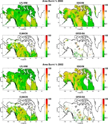
which shows the burned areas in 2000 and 2002 over North America according to the three models and GFED-BA. The data indicate that 2002 was a much more severefire year in North America than 2000, mainly because of the Long Creek Fire in Alaska andfires in Quebec, and the 2 years ex-hibit quite different spatial patterns, but these differences are not captured by the models. While burns occur in only a small proportion of GFED-BA grid cells each year, and large fractions of some cells are burned, in the models, a small frac-tion of almost every grid cell burns every year (except for most grid cells north of 65°N in CLM4CN, where fire is not permitted).

[37] This discrepancy arises because the treatment offire in

the models is deterministic, while in practice,fire is stochas-tic. For example, in Canada, largefires made up only 3% of the totalfires occurring from 1959 to 1999 but contributed 97% of the burned area [Stocks et al., 2002]. These rare events follow the law of small numbers, and their occurrence Figure 3. Annualfire emissions (in Tg C yr 1) from northern high latitudes averaged over 1981–2006 for

the three models.

Table 2. Annual Carbon Emissions (Tg C yr 1) Averaged Over 1981–2006 for the Three Models Over North America, Eurasia, and All Northern High Latitudesa

Fire Emissions (Tg C yr 1) LPJ-WM SDGVM CLM4CN GFED

North America 192 71 55 56

Eurasia 471 201 110 144

Boreal and Arctic 663 272 164 200

a

is usually modeled by a Poisson distribution [Jiang et al., 2012;Mandallaz and Ye, 1997]. The lack of such a random component infire occurrence is not apparent when FRI or an-nual average burn is used to compare model outputs with data. [38] The total burned areas of the panboreal region, North

America, and Eurasia estimated by GFED-BA for 1997– 2006, MODIS-BA for 2002–2006, and the three models for 1981–2006 are compared in Figure 6 (left). Since GFED-BA exploits MODIS-GFED-BA, these two observational data sets correlate well over their common time period from 2002 to 2009, though MODIS-BA produces more burned area in Eurasia and less in North America [Giglio et al., 2010;

van der Werf et al., 2010]. In contrast, none of the models shows any significant correlation with GFED-BA for the overlapping period 1997–2006, either by continent or glob-ally, as has previously been noted for CLM4CN over the panboreal region [Kloster et al., 2010]. The observations also exhibit markedly greater interannual variability than the model values, especially LPJ-WM and CLM4CN. Hence, the mean values of the four estimates shown in Table 3 do not really capture the model-data differences; for example, the global mean burned area in GFED-BA lies between the values from the three models, but values in some individual years are high and close to those from SDGVM, while other

years give much lower values that are closer to those from the other two models. CLM4CN and LPJ-WM produce similar burned areas, with those from LPJ-WM always being higher, while SDGVM consistently produces values that are 50–100% larger, globally and in each continent.

3.3. Estimated Fire Emissions

[39] Comparisons between the four time series of burned

area and emissions for GFED and the three models exhibit two striking differences (Figure 6):

[40] 1. Despite LPJ-WM producing burned area that is

comparable with CLM4CN and much less than SDGVM, Figure 4. Percentage of annually burned area in logarithmic scale at northern high latitudes averaged over

1981–2006 for the three models and over 1997–2009 for GFED-BA.

Table 3. Annual Burned Area (in Mha yr 1) Averaged Over 1981–2006 for the Three Models Over North America, Eurasia, and All Northern High Latitudesa

Burned Area (Mha yr 1) LPJ-WM SDGVM CLM4CN GFED-BA

North America 3.4 5.4 2.9 2.04

Eurasia 7.2 11.8 5.8 10.0

Boreal and Arctic 10.6 17.2 8.7 12.04

a

its estimates of emissions are higher than those from the other two models by a factor 2 or greater, both globally and in each continent.

[41] 2. Although SDGVM gives much greater burned area

than either of the other models, its emission estimates are comparable to those of CLM4CN in North America and only about 30% higher than those of CLM4CN in Siberia.

[42] It should be noted that although the burned area in

GFED is derived from observations, GFED emissions are calculated using the CASA model; hence, all four emission estimates in Figure 6 are model based. It can also be seen that the mean emissions from GFED, CLM4CN, and SDGVM are comparable, but LPJ-WM gives a much higher value (Table 2).

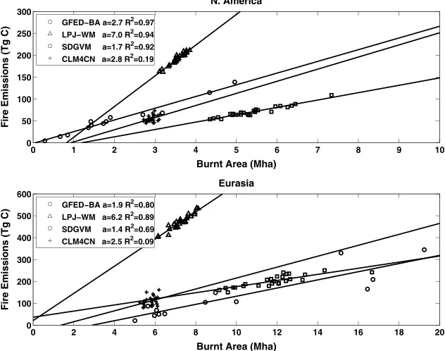
[43] The relation between burned area and emissions is a

function of available fuel (biomass, litter, and carbonaceous soils) and the effectiveness with which fires consume this fuel, so it can be relatively complex at the local scale. However, at continental scales, a fairly simple picture emerges, as can be seen from Figure 7, which plots emissions

against burned area in North America and Eurasia for each year from 1981 to 2006 for the three models and emissions from GFED against burned area from GFED-BA for 1997– 2009. A best linearfit to each plot is also shown, whose slope gives the mean emissions per unit area burned, and is a func-tion of combusfunc-tion completeness and the fuel load available in each model.

[44] Sharp differences infire emissions are seen between

all four estimates. Apart from CLM4CN, annual emissions are almost linearly related to burned area. The emissions per unit burned area are much higher for LPJ-WM than for the other models and larger for GFED than SDGVM in both North America and in Eurasia, while the R2 value for CLM4CN is too low to assign any useful meaning to the calcu-lated slope. All the estimates indicate that fires in North America produce more emissions per unit area than in Eurasia; this agrees with studies by Wooster and Zhang

[2004], based on measurements of Fire Radiative Power, and has been attributed to the predominance of crown or canopy fires in North America, while crawling or surfacefires tend to Figure 5. Percentage of burned area in logarithmic scale in 2000 and 2002 over North America for the

dominate in Eurasia. With the exception of CLM4CN, theR2

values are very high in North America but smaller in Eurasia; this may be because manyfires in Eurasia occur at latitudes from 50°N to 65°N (Figure 4), where, even though herbaceous and tree cover are equally present overall, they are highly

clustered, with herbaceous cover dominating the western part and forests the eastern. The difference in biomass between the two types causes a partial decoupling of burned area and fire emissions, a phenomenon which is also observed at global scale [van der Werf et al., 2006].

Figure 6. (left) Total area burned per year (Mha yr 1) for the northern high latitudes, North America, and Eurasia as calculated by the three models and given by GFED-BA and MODIS-BA. (right) The corre-spondingfire emissions (Tg C yr 1) for the models and GFED.

Figure 7. Regression of annual fire emissions (Tg C) against annual burned area (Mha) for the three DVMs (1981–2006) and GFED (1997–2009) over North America and Eurasia. The slope of the regression,

a(Tg C/Mha), and theR2_coef

4. Discussion

[45] Two questions immediately arise from the results in

section 3:

[46] 1. What is the explanation for the large differences

be-tween different estimates offire emissions, and are there data to help clarify which model best represents thefire process? [47] 2. Do the striking differences between the statistical

properties of observed and modeled burned areas have conse-quences for other properties of the system, such as NBP and biomass?

4.1. Differences Between Model Parameterizations of Fire Emissions and Their Consequences

[48] The different model estimates of carbon emissions

seen in section 3.3 do not stem from fundamental differences between the models, since they all use an approach that weights the area burned by the available fuel load while fac-toring in variables that define the combustion process. However, the models make different assumptions about the fuel load and combustion completeness (defined as the frac-tion of burnt fuel that is emitted to the atmosphere), as sum-marized in Table 4. In addition, the models assign a fire mortality factor to each PFT, which defines the fraction of in-dividuals in the burned area that will be affected byfire. LPJ-WM and CLM4CN assign similar values to this factor for each of the tree PFTs and the value of 1 for herbaceous cover, while SDGVM assigns the value of 1 to all PFTs.

[49] SDGVM treats only aboveground biomass as fuel,

whereas LPJ-WM and CLM4CN include belowground bio-mass and litter. Hence, SDGVM has a much smaller fuel load and yields much lower carbon emissions, despite burning around 60–100% more area (see Table 3 and Figure 7). LPJ-WM and CLM4CN produce similar burned areas, but LPJ-WM yields carbon emissions that are more than 4 times greater. A major factor in this discrepancy comes from burning of litter, which accounts for 56% of the emissions (372 Tg C yr 1) in LPJ-WM but only 30% (50 Tg C yr 1) in CLM4CN. This large difference arises partly from the much larger litter pool in LPJ-WM (an average value of 103 Pg C compared with 21 Pg C for CLM4CN); LPJ-WM also treats litter as a single pool with a combustion completeness of 100%, while CLM4CN assigns different values of combustion completeness to coarse woody debris, leaf litter, etc. In partic-ular, in CLM4CN, the litter mainly consists of coarse woody debris, for which the combustion completeness is only 40%.

[50] Emissions from biomass burning are also larger in

LPJ-WM than CLM4CN (average values of 290 Tg C yr 1 and 114 Tg C yr 1_{, respectively). This arises partly from} LPJ-WM having 9.27 × 104Tg C of biomass compared to 7.47 × 104_{Tg C in CLM4CN, but more important is that}

LPJ-WM assumes complete combustion of aboveground and belowground biomass, while CLM4CN completely burns the leaves andfine roots but assigns a combustion completeness factor of only 20% to the stem and coarse roots [Oleson et al., 2010]. Note that the more complex CLM4CN scheme is similar to that adopted by CASA; hence, the large differ-ences between them (Figure 7) reflect the very low variability in burned area in CLM4CN, together with differences in the carbon pools estimated in the models. However, we do not have access to the details of the CASA carbon calculations un-derlying the GFED estimates and hence cannot provide quan-titative assessment of these differences.

[51] Overall, it is clear that the models disagree markedly

about the relative importance of emissions from litter and from biomass: LPJ-WM produces 28% more emissions from litter than biomass, CLM4CN produces 66% less, while the whole of the 272 Tg C yr 1_{emitted by}

fire from SDGVM comes from burning aboveground biomass. This immedi-ately raises the question of whether there are empirical data on the combustion completeness of carbon pools in northern high latitudes that can be used to test the models.

[52] As noted byvan der Werf et al. [2010], the accuracy of

fire emission estimates is limited by the available information on combustion completeness and emission factors, which is sparse and unsystematic and typically refers to specific fire events [Mack et al., 2011] or experimental fires [FIRESCAN, 1996]. The available studies show that consump-tion of both biomass and litter byfire varies greatly, depending on environmental factors, the types offire, and the type of eco-system. Several investigators have parameterized combustion completeness according tofire severity andfire type. For exam-ple, inConard and Ivanova[1997], the combustion complete-ness values for both understorey vegetation and litter are taken to be 100% in high-severity canopyfires; 90% and 50%, re-spectively, for high-severity surfacefires; and 50% and 10%, respectively, for low-severity surfacefires. About 15% of the woody biomass is consumed in canopyfires, but this concerned a specific tree species.Soja et al. [2004] reported typical values of soil organic matter consumed by high-, medium-, and low-severityfires as 5, 2, and 1 cm in a standard scenario and 10, 4, and 2 cm in an extreme scenario.

[53] Although sparse, these observations suggest that the

more complete parameterization of fuel load in CLM4CN is likely to be more realistic. However, the data also indicate that combustion completeness andfire severity are not inde-pendent, as assumed by the DVMs (though not by CASA, in which combustion completeness is proportional to soil mois-ture, which is used as a proxy offire severity). In recognition of this,Thonicke et al. [2010] released an improved version of the LPJ model which used a newfire model (SPITFIRE) that linked fire severity to litter combustion completeness. Table 4. Definitions of Fuel Load and Combustion Completeness in the Three DVMs and in the CASA Model Used by GFEDa

LPJ-WM SDGVM CLM4CN GFED (CASA)

Fuel load AGB, BGB, and litter AGB only AGB, BGB, and litter AGB, BGB, and litter Combustion completeness Biomass: 100% AGB: 80% Leaves andfine roots: 100% Leaves: 80–100%

Litter: 100% Stem and coarse roots: 20% Stems: 20–40% Litter: 100% Fine litter: 90–100% Woody debris: 40% Woody debris: 40–60%

Litter: 100%

However, this still underestimated the interannual variability of burned area in the boreal zone, indicating that steps are still needed to represent more accurately the stochastic nature of fires. In addition, this version of the model does not include organic soils, boreal PFTs, or permafrost, unlike LPJ-WM, so it was not appropriate for this study.

4.2. The Effects of Improving the Spatiotemporal Description of Burned Area on Model Estimates of High-Latitude Processes

[54] Section 2.3 described modifications to SDGVM and

LPJ-WM that make the statistical properties of their esti-mates of burned area conform more closely to observations. The need to consider modifications to both models stems from the suitability of each model for the issues addressed be-low. SDGVM has a particularly simple relation betweenfire and emissions, so it is well suited to investigating the role of fire in the interannual variability of NBP. Unlike SDGVM, LPJ-WM incorporates permafrost dynamics, so it is suitable for investigatingfire-permafrost links.

4.2.1. The Effects of Enhanced Interannual Variability of Burned Area on NBP and Biomass

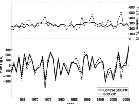
[55] Increasing the variability in burned area to be

consis-tent with observations (see section 2.3.1) causes an increase from 30 Tg yr 1_{to 79 Tg yr} 1_{in the interannual variability} of thefire emissions calculated by SDGVM over the period 1960–2006. There is an associated increase in the interannual variability of NBP, but only by 15%, and it is still dominated by climate variability. Only 22% of the adjusted NBP vari-ance can be attributed to the varivari-ance of the adjusted fire emissions, and there is little correlation between NBP and the size of the emissions (see Figure 8). These model-based results imply thatfire/nonfire years are not the main determi-nant of whether a given year will be a CO2sink or a source, andfire emissions are not the major driver of the observed variability of land-atmosphere carbon exchange. A similar conclusion would be drawn for CLM4CN and GFED, be-cause both have significantly smaller total fire emissions than SDGVM (see Table 2). This is consistent with thefi nd-ing ofPrentice et al. [2011], also model based, that the CO2 fluxes produced by GFED during 1997–2005 would have

contributed only a third of the variability in total global CO2flux inferred from atmospheric inversion, despite earlier studies postulating that biomass burning is the major compo-nent in land-atmosphere carbon flux anomalies [Nevison et al., 2008;Patra et al., 2005]. Nevertheless, our conclusion relies on the model used to calculatefire emissions and may have been different for the much higher values from LPJ-WM; we did not pursue this as these are probably too high (see Figure 6). This emphasizes the need for more direct mea-surements of emissions, as such are increasingly becoming available from measurements of Fire Radiative Power [Kaiser et al., 2012].

[56] The effects on biomass are illustrated for the

panboreal region in Figure 9, which shows the difference be-tween SDGVM and SDGVM* as a percentage of the unmodified value. Although the overall effect is to slightly reduce overall biomass, the modifiedfire regime leads to a complex pattern of increases and decreases in the local mean biomass, essentially because it causes the occurrence of very large fires destroying large parts of the vegetation in many grid cells in some years, thus altering the age structure in the forest component of vegetation. This pattern of heteroge-neity varies though time, but its statistical properties are sta-ble and does not give rise to major changes in the mean NBP. 4.2.2. The Effects of Modi_fied Burned Area Statistics on Permafrost

[57] In a boreal Alaskan forest underlain by permafrost,

[58] The modification to LPJ-WM described in section

2.3.2 changes this situation by allowing large fractions of some grid cells to burn. Since 100% of the insulating litter layer is removed in the burned fraction (see Table 4), this has significant effects on soil temperature and hence on per-mafrost. Furthermore, removal of canopy byfire alters the ra-diation budget: for example, prior to disturbance, 30–65% of incoming solar radiation reaches the forest floor in black spruce forests [Slaughter, 1983], while after afire, it exceeds 90% [Kasischke et al., 1995]. This cannot be simulated by the current version of LPJ-WM, which lacks a full radiation balance in its energy calculations. Hence, a rough approxi-mation was made in which the input air temperature, which acts as an upper boundary condition for the heat diffusion equation, was increased in the year after afire and decreased as an exponential function of tree cover. This simulates an in-crease of leaf area index and associated attenuation of radia-tion according to Beer-Lambert’s law.

[59] The cumulative effect of these two modifications is

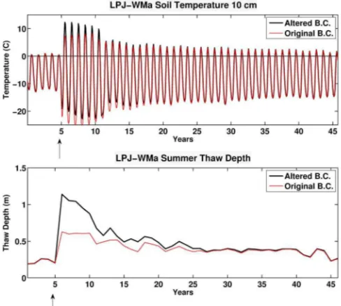
il-lustrated by Figure 10, in which the upper plot shows the monthly soil temperatures at a depth of 10 cm calculated by LPJ-WMa at a location dominated by deciduous needle-leaved forest in northern Siberia after afire with 99% fraction

of burn. Following the disturbance, the model initially sets herbaceous cover as the dominant PFT in the grid cell, while the needle-leaved PFT becomes dominant after 15 years. Figure 10 shows that the removal of litter and its subsequent damping effect increases the monthly variability of soil tem-perature as it becomes more susceptible to air temtem-perature and its periodicfluctuations. Since summer soil temperatures now exceed 0°C, summer thaw depth increases by over 1.0 m and requires more than 60 years to return to its predisturbed value. These values are closer to field measurements than when the boundary conditions were unchanged, in which case the increase in maximum thaw depth due to loss of litter is less than 0.5 m, although the time to recovery of the origi-nal temperature conditions is the same (see Figure 10).

[60] Although the modifications to LPJ-WM provide more

realistic simulations of permafrost dynamics following afire by generating greater thaw depths, the current model formu-lation cannot capture the full extent offire-permafrost inter-actions, e.g., thaw depth increases for several years after a fire, not just in the immediately following year [MacKay, 1970; Yoshikawa et al., 2002]. Achieving this is hindered by the fact thatfire is not treated as a continuous process in the model; instead, all the burn effects, e.g., loss of canopy Figure 9. Percentage difference in biomass between modified and unmodified SDGVM calculations, i.e.,

100 × (SDGVM* SDGVM)/SDGVM, averaged over 1997–2006.

and litter, are imposed on January 1 of each year. Hence, the expected thawing of permafrost after a summer fire is not properly represented. Clearly, the radiation balance also needs to be treated properly, rather than in the ad hoc ap-proach used here to illustrate its importance. Furthermore, the effects of localized intensefire events that occupy only a small part of a grid cell are not properly represented because of the averaging across grid cells used by models, even though these subgrid cell events are likely to form an impor-tant driver of the dynamics of permafrost.

5. Conclusions

[61] Fire is an endemic process at high latitudes, connected

to a range of other land surface properties, such as land cover, biomass, and permafrost, and intimately linked to the carbon balance of the high-latitude land surface. Much of our current understanding of these links and their climate consequences is through land surface models, so it is essential to ensure that the process representations and parameterizations in these models are consistent with observations; only then will they be able to provide trustworthy predictions for a changing climate. Over the vast panboreal region, a key source of in-formation on fire is satellite data. Comparisons between satellite-based burned area data from the Global Fire Emissions Database (GFED) and three DVMs (LPJ-WM, CLM4CN, and SDGVM) indicate that all models fail to rep-resent the observed spatial and temporal properties of thefire regime and that there are large discrepancies between models and data with regard to average annual burned area. Although the three DVMs give comparable values of the boreal net bi-ome production (NBP),fire emissions are found to differ by a factor 4 between the models, because of widely different es-timates of burned area and because of different parameteriza-tions of the fuel load and combustion process. Including a more realistic representation of thefire regime in the models shows that for northern high latitudes, (i) severefire years do not coincide with CO2source years or vice versa; (ii) increas-ing the interannual variability of burned area to be consistent with data increases the interannual variability of NBP, but cli-mate variability remains the main factor determining its mag-nitude; and (iii) overall biomass values alter only slightly, but the spatial distribution of biomass exhibits changes. It must be stressed that these conclusions are derived using model es-timates offire emissions, which this study has demonstrated to be problematic; thus, they should not be considered robust un-til verified by measurements or by models with considerably improved representation of boreal fire processes. We also demonstrate that it is crucial to alter the current representations offire occurrence and severity in land surface models if the links between permafrost andfire are to be captured, in partic-ular, the dynamics of permafrost properties, such as active layer depth. This is especially important if models are to be used to predict the effects of a changing climate, because of the consequences of permafrost changes for greenhouse gas emissions, hydrology, and land cover.

[62] This study highlights two areas where further work is

clearly needed. The first is improved experimental data on fire processes at high latitudes, with regard to the pools entrained infire events and the combustion completeness of these pools. Lack of knowledge about these factors is a major source of uncertainty in model estimates, both in the DVMs

and in GFED (through CASA). This is not a fundamental weakness of the models, only of the parameter settings within their representations of fire, particularly for CLM4CN and CASA, which already contain a comprehensive description of the pools contributing to the fuel load.

[63] However, there are fundamental limitations in the

cur-rent ways that fire occurrence and fire severity are repre-sented in the models, with follow-on consequences for the need for better energy balance representations if models are to be capable of predicting permafrost dynamics and associ-ated effects on greenhouse gas emissions, hydrology, and land cover. Removing these limitations constitutes the sec-ond major area where further work is needed. This has two components:

[64] 1. Models for fire occurrence and severity that more

realistically capture the observed high variability in space and time of high-latitudefires are formulated. A purely statis-tical approach has been used in this paper to assess the impor-tance of representing such variability; its most significant effect, within the limits of our study, appears to be on perma-frost. However, for predictive purposes under changing cli-mate, a more mechanistic approach may be preferable, with a stochastic component related to ignition probabilities. An associated issue is that most current models simply average fire-affected areas back into the overall vegetation structure in a grid cell, which dilutes their effect. Internal grid cell het-erogeneity is required if the effects of smaller severefires on vegetation and soil dynamics are to be correctly represented. [65] 2. More complete models for energy balance afterfire

are needed to include the effects of both heat diffusion and ra-diation. Failure to include the latter leads to errors in the pre-dicted mean soil temperature and to large underestimates of the time for permafrost to recover afterfire. This may also re-quire better representations of vegetation, for example, to in-clude the thermal consequences of a moss layer.

[66] Acknowledgments. This study was carried out as part of European Union FP7-SPACE-2009-1 Collaborative Project 242446, MONARCH-A: Monitoring and assessing regional climate change in high latitudes and the Arctic. The authors would like to thank the partners of the TRENDY project for data access to model runs. We would also like to thank Rita Wania for access to the code and technical assistance on the LPJ-WM model.

References

Arino, O., S. Casadio, and D. Serpe (2012), Global night-timefire season timing andfire count trends using the ATSR instrument series,Remote Sens. Environ.,116, 226–238, doi:10.1016/j.rse.2011.05.025.

Baker, D. F., et al. (2006), TransCom 3 inversion intercomparison: Impact of transport model errors on the interannual variability of regional CO2 fluxes, 1988–2003, Global Biogeochem. Cycles, 20, GB1002, doi:10.1029/2004gb002439.

Bowman, D. M. J. S., et al. (2009), Fire in the Earth system, Science, 324(5926), 481–484, doi:10.1126/science.1163886.

Brown, R. J. E. (1983), Effects offire on permafrost ground thermal regime, inThe Role of Fire in Northern Circumpolar Ecosystems, edited by R. W. Wein and D. A. MacLean, pp. 97–110, John Wiley, New York. Christensen, J. H., B. Hewitson, A. Busuioc, A. Chen, X. Gao, I. Held,

R. Jones, and R. K. Kolli (2007), Regional Climate Projections, inClimate Change 2007: The Physical Science Basis. Contribution of Working Group I to the Fourth Assessment Report of the Intergovernmental Panel on Climate Change, edited by S. Solomon, et al., pp. 847–940, Cambridge University Press, Cambridge, U.K.

Collins, W. D., et al. (2006), The Community Climate System Model version 3 (CCSM3),J. Clim.,19(11), 2122–2143.

Conard, S. G., and G. A. Ivanova (1997), Wildfire in Russian boreal forests

Corell, R. (2005), Arctic climate impact assessment,Bull. Am. Meteorol. Soc.,86(6), 860–861.

Cox, P., and D. Stephenson (2007), Climate change—A changing climate for prediction, Science, 317(5835), 207–208, doi:10.1126/ science.1145956.

Cramer, W., et al. (2001), Global response of terrestrial ecosystem structure and function to CO2 and climate change: Results from six dynamic global vegetation models,Global Change Biol.,7(4), 357–373.

Dyrness, C. T., L. A. Viereck, and K. Van Kleave (1986), Fire in taiga com-munities of interior Alaska, inEcological Series: Forest Ecosystems in the Alaskan Taiga, edited by K. Van Cleave, pp. 74–86, Springer, New York. FIRESCAN (1996), Fire Research Campaign Asia-North, in Biomass Burning and Global Change, edited by J. S. Levine, pp. 848–873, MIT Press, Cambridge, Mass.

Flannigan, M. D., and C. E. Vanwagner (1991), Climate change and wildfire in Canada,Can. J. For. Res.,21(1), 66–72, doi:10.1139/X91-010. Friedlingstein, P., et al. (2006), Climate-carbon cycle feedback analysis: Results

from the C(4)MIP model intercomparison,J. Clim.,19(14), 3337–3353. GCOS (2004),Implementation Plan for the Global Observing System

for Climate in Support of the UNFCCC, GCOS–92, WMO Technical Document No. 1219WMO, Geneva, Switzerland.

GCOS (2010),Implementation Plan for the Global Observing System for Climate in Support of the UNFCCC (2010 Update), WMO, Geneva. Gerten, D., S. Schaphoff, U. Haberlandt, W. Lucht, and S. Sitch (2004),

Terrestrial vegetation and water balance—Hydrological evaluation of a dynamic global vegetation model,J. Hydrol.,286(1–4), 249–270, doi:10.1016/j.jhydrol.2003.09.029.

Giglio, L. (2010),MODIS Collection 5 Active Fire Product User’s Guide, Version 2.4, Department of Geography, University of Maryland, Md. Giglio, L., J. T. Randerson, G. R. van der Werf, P. S. Kasibhatla,

G. J. Collatz, D. C. Morton, and R. S. DeFries (2010), Assessing variabil-ity and long-term trends in burned area by merging multiple satellitefire products,Biogeosciences,7(3), 1171–1186.

Gurney, K. R., et al. (2003), TransCom 3 CO2 inversion intercomparison: 1. Annual mean control results and sensitivity to transport and priorflux in-formation,Tellus, Ser. B,55(2), 555–579.

Jiang, Y., Q. Zhuang, and D. Mandallaz (2012), Modeling largefire frequency and burned area in Canadian terrestrial ecosystems with Poisson models, Environ. Model. Assess.,17, 483–493, doi:10.1007/s10666-012-9307-5. Kaiser, J. W., et al. (2012), Biomass burning emissions estimated with a

globalfire assimilation system based on observedfire radiative power, Biogeosciences,9(1), 527–554, doi:10.5194/bg-9-527-2012.

Kanamitsu, M., W. Ebisuzaki, J. Woollen, S. K. Yang, J. J. Hnilo, M. Fiorino, and G. L. Potter (2002), Ncep-Doe Amip-Ii Reanalysis (R-2),Bull. Am. Meteorol. Soc.,83(11), 1631–1643, doi:10.1175/Bams-83-11-1631. Kasischke, E. S., N. L. Christensen, and B. J. Stocks (1995), Fire, global

warming, and the carbon balance of boreal forests,Ecol. Appl.,5(2), 437–451.

Kloster, S., N. M. Mahowald, J. T. Randerson, P. E. Thornton, F. M. Hoffman, S. Levis, P. J. Lawrence, J. J. Feddema, K. W. Oleson, and D. M. Lawrence (2010), Fire dynamics during the 20th century simulated by the Community Land Model, Biogeosciences, 7(6), 1877–1902, doi:10.5194/bg-7-1877-2010.

Lawrence, D. M., and A. G. Slater (2008), Incorporating organic soil into a global climate model, Clim. Dyn., 30(2–3), 145–160, doi:10.1007/ s00382-007-0278-1.

Lawrence, D. M., A. G. Slater, V. E. Romanovsky, and D. J. Nicolsky (2008), Sensitivity of a model projection of near-surface permafrost degradation to soil column depth and representation of soil organic matter,J. Geophys. Res.,113, F02011, doi:10.1029/2007jf000883.

Lawrence, D. M., et al. (2011), Parameterization improvements and functional and structural advances in Version 4 of the Community Land Model, J. Adv. Model. Earth Syst.,3, M03001, doi:10.1029/2011ms000045. Le Quere, C., et al. (2009), Trends in the sources and sinks of carbon dioxide,

Nat. Geosci.,2(12), 831–836, doi:10.1038/ngeo689.

Mack, M. C., M. S. Bret-Harte, T. N. Hollingsworth, R. R. Jandt, E. A. G. Schuur, G. R. Shaver, and D. L. Verbyla (2011), Carbon loss from an unprecedented Arctic tundra wildfire,Nature,475(7357), 489–492, doi:10.1038/nature10283.

MacKay, J. R. (1970), Disturbances to the tundra and forest tundra environ-ments of the western Arctic,Can. Geotech. J.,7(4), 420–432.

Mandallaz, D., and R. Ye (1997), Prediction of forestfires with Poisson models,Can. J. For. Res.,27(10), 1685–1694.

McGuire, A. D., J. M. Melillo, D. W. Kicklighter, and L. A. Joyce (1995), Equilibrium responses of soil carbon to climate change: Empirical and process-based estimates,J. Biogeogr.,22(4–5), 785–796.

McGuire, A. D., L. G. Anderson, T. R. Christensen, S. Dallimore, L. D. Guo, D. J. Hayes, M. Heimann, T. D. Lorenson, R. W. Macdonald, and N. Roulet (2009), Sensitivity of the carbon cycle in the Arctic to climate change,Ecol. Monogr.,79(4), 523–555.

Mitchell, T. D., and P. D. Jones (2005), An improved method of constructing a database of monthly climate observations and associated high-resolution grids,Int. J. Climatol.,25(6), 693–712, doi:10.1002/joc.1181.

Nevison, C. D., N. M. Mahowald, S. C. Doney, I. D. Lima, G. R. Van der Werf, J. T. Randerson, D. F. Baker, P. Kasibhatla, and G. A. McKinley (2008), Contribution of ocean, fossil fuel, land biosphere, and biomass burning carbonfluxes to seasonal and interannual variability in atmospheric CO2, J. Geophys. Res.,113, G01010, doi:10.1029/2007JG000408.

Oleson, K. W., et al. (2010),Technical Description of Version 4.0 of the Community Land Model, NCAR Technical Note 47, 257 pp. Boulder, Colo. NCAR.

Patra, P. K., M. Ishizawa, S. Maksyutov, T. Nakazawa, and G. Inoue (2005), Role of biomass burning and climate anomalies for land-atmosphere car-bon fluxes based on inverse modeling of atmospheric CO2, Global Biogeochem. Cycles,19, GB3005, doi:10.1029/2004gb002258. Pechony, O., and D. T. Shindell (2010), Driving forces of global wildfires

over the past millennium and the forthcoming century,Proc. Natl. Acad. Sci. U. S. A.,107(45), 19,167–19,170, doi:10.1073/pnas.1003669107. Piao, S. L., J. Y. Fang, P. Ciais, P. Peylin, Y. Huang, S. Sitch, and T. Wang

(2009), The carbon balance of terrestrial ecosystems in China,Nature, 458(7241), 1009–1013, doi:10.1038/Nature07944.

Potter, C. S., J. T. Randerson, C. B. Field, P. A. Matson, P. M. Vitousek, H. A. Mooney, and S. A. Klooster (1993), Terrestrial ecosystem produc-tion—A process model-based on global satellite and surface data,Global Biogeochem. Cycles,7(4), 811–841.

Prentice, I. C., D. I. Kelley, P. N. Foster, P. Friedlingstein, S. P. Harrison, and P. J. Bartlein (2011), Modelingfire and the terrestrial carbon balance, Global Biogeochem. Cycles,25, GB3005, doi:10.1029/2010gb003906. Quegan, S., C. Beer, A. Shvidenko, I. McCallum, I. C. Handoh, P. Peylin,

C. Rodenbeck, W. Lucht, S. Nilsson, and C. Schmullius (2011), Estimating the carbon balance of central Siberia using a landscape-ecosystem approach, atmospheric inversion and Dynamic Global Vegetation Models,Global Change Biol.,17(1), 351–365, doi:10.1111/j.1365-2486.2010.02275.x. Roberts, G. J., and M. J. Wooster (2008), Fire detection andfire

characteri-zation over Africa using Meteosat SEVIRI,IEEE Trans. Geosci. Remote Sens.,46(4), 1200–1218, doi:10.1109/Tgrs.2008.915751.

Rödenbeck, C., S. Houweling, M. Gloor, and M. Heimann (2003), CO2 flux history 1982–2001 inferred from atmospheric data using a global inversion of atmospheric transport,Atmos. Chem. Phys.,3, 1919–1964.

Roy, D. P., L. Boschetti, C. O. Justice, and J. Ju (2008), The collection 5 MODIS burned area product—Global evaluation by comparison with the MODIS activefire product,Remote Sens. Environ.,112(9), 3690–3707, doi:10.1016/j.rse.2008.05.013.

Serreze, M. C., and J. A. Francis (2006), The arctic amplification debate, Clim. Change,76(3–4), 241–264, doi:10.1007/s10584-005-9017-y. Sitch, S., et al. (2003), Evaluation of ecosystem dynamics, plant geography

and terrestrial carbon cycling in the LPJ dynamic global vegetation model, Global Change Biol.,9(2), 161–185.

Slaughter, C. W. (1983), Summer shortwave radiation at a subarctic forest site,Can. J. For. Res.,13(5), 740–746.

Soja, A. J., W. R. Cofer, H. H. Shugart, A. I. Sukhinin, P. W. Stackhouse, D. J. McRae, and S. G. Conard (2004), Estimatingfire emissions and dis-parities in boreal Siberia (1998–2002),J. Geophys. Res.,109, D14S06, doi:10.1029/2004jd004570.

Stocks, B. J., et al. (1998), Climate change and forestfire potential in Russian and Canadian boreal forests,Clim. Change,38(1), 1–13.

Stocks, B. J., et al. (2002), Large forest fires in Canada, 1959–1997, J. Geophys. Res.,108(D1), 8149, doi:10.1029/2001JD000484.

Street, L. E., P. C. Stoy, M. Sommerkorn, B. J. Fletcher, V. L. Sloan, T. C. Hill, and M. Williams (2012), Seasonal bryophyte productivity in the sub-Arctic: A comparison with vascular plants,Funct. Ecol.,26(2), 365–378, doi:10.1111/j.1365-2435.2011.01954.x.

Tarnocai, C., J. G. Canadell, E. A. G. Schuur, P. Kuhry, G. Mazhitova, and S. Zimov (2009), Soil organic carbon pools in the northern circumpolar permafrost region, Global Biogeochem. Cycles, 23, GB2023, doi:10.1029/2008gb003327.

Thonicke, K., S. Venevsky, S. Sitch, and W. Cramer (2001), The role offire disturbance for global vegetation dynamics: Couplingfire into a Dynamic Global Vegetation Model, Global. Ecol. Biogeogr., 10(6), 661–677.

Thonicke, K., A. Spessa, I. C. Prentice, S. P. Harrison, L. Dong, and C. Carmona-Moreno (2010), The influence of vegetation,fire spread and fire behaviour on biomass burning and trace gas emissions: Results from a process-based model,Biogeosciences,7(6), 1991–2011, doi:10.5194/ bg-7-1991-2010.

Tjiputra, J. F., K. Assmann, M. Bentsen, I. Bethke, O. H. Ottera, C. Sturm, and C. Heinze (2010), Bergen Earth system model (BCM-C): Model de-scription and regional climate-carbon cycle feedbacks assessment, Geosci. Model Dev.,3(1), 123–141.

Turetsky, M., K. Wieder, L. Halsey, and D. Vitt (2002), Current disturbance and the diminishing peatland carbon sink,Geophys. Res. Lett.,29(11), 1526, doi:10.1029/2001gl014000.

Viereck, L. A. (1983), The effects offire in black spruce ecosystems of Alaska and northern Canada, inThe Role of Fire in Northern Circumpolar Ecosystems, edited by R. W. Wien and D. A. MacLean, pp. 201–220, Wiley & Sons Ltd, Chichester, UK.

Wania, R., I. Ross, and I. C. Prentice (2009), Integrating peatlands and permafrost into a dynamic global vegetation model: 1. Evaluation and sensitivity of physical land surface processes, Global Biogeochem. Cycles,23, GB3014, doi:10.1029/2008gb003412.

van der Werf, G. R., J. T. Randerson, L. Giglio, G. J. Collatz, P. S. Kasibhatla, and A. F. Arellano (2006), Interannual variability in global biomass burning emissions from 1997 to 2004,Atmos. Chem. Phys.,6, 3423–3441.

van der Werf, G. R., J. T. Randerson, L. Giglio, G. J. Collatz, M. Mu, P. S. Kasibhatla, D. C. Morton, R. S. DeFries, Y. Jin, and T. T. van Leeuwen (2010), Globalfire emissions and the contribution of deforestation, savanna,

forest, agricultural, and peatfires (1997–2009),Atmos. Chem. Phys.,10(23), 11,707–11,735, doi:10.5194/acp-10-11707-2010.

Woodward, F. I., and M. R. Lomas (2004), Vegetation dynamics— simulat-ing responses to climatic change,Biol. Rev.,79(3), 643–670, doi:10.1017/ S1464793103006419.

Woodward, F. I., T. M. Smith, and W. R. Emanuel (1995), A Global land pri-mary productivity and phytogeography model, Global Biogeochem. Cycles,9(4), 471–490.

Wooster, M. J., and Y. H. Zhang (2004), Boreal forestfires burn less in-tensely in Russia than in North America, Geophys. Res. Lett., 31, L20505, doi:10.1029/2004GL020805.

Wooster, M. J., G. Roberts, G. L. W. Perry, and Y. J. Kaufman (2005), Retrieval of biomass combustion rates and totals fromfire radiative power observations: FRP derivation and calibration relationships between biomass consumption andfire radiative energy release,J. Geophys. Res., 110, D24311, doi:10.1029/2005jd006318.

Wotton, B. M., and M. D. Flannigan (1993), Length of thefire season in a changing climate,For. Chron.,69(2), 187–192.