White Rose Research Online URL for this paper:
http://eprints.whiterose.ac.uk/106156/
Version: Accepted Version
Article:
Zhao, X, Wang, H orcid.org/0000-0002-2281-5679 and Komura, T (2014) Indexing 3d
scenes using the interaction bisector surface. ACM Transactions on Graphics (TOG), 33
(3). 22. ISSN 0730-0301
https://doi.org/10.1145/2574860
© ACM, 2014. This is the author's version of the work. It is posted here by permission of
ACM for your personal use. Not for redistribution. The definitive version was published in
ACM Transactions on Graphics (TOG) , 33 (3), May 2014,
http://doi.acm.org/10.1145/2574860. Uploaded in accordance with the publisher's
self-archiving policy.
[email protected]
https://eprints.whiterose.ac.uk/
Reuse
Unless indicated otherwise, fulltext items are protected by copyright with all rights reserved. The copyright
exception in section 29 of the Copyright, Designs and Patents Act 1988 allows the making of a single copy
solely for the purpose of non-commercial research or private study within the limits of fair dealing. The
publisher or other rights-holder may allow further reproduction and re-use of this version - refer to the White
Rose Research Online record for this item. Where records identify the publisher as the copyright holder,
users can verify any specific terms of use on the publisher’s website.
Takedown
If you consider content in White Rose Research Online to be in breach of UK law, please notify us by
Xi Zhao
University of Edinburgh He Wang
University of Edinburgh Taku Komura
University of Edinburgh
The spatial relationship between different objects plays an important role in defining the context of scenes. Most previous 3D classification and retrieval methods take into account either the individual geometry of the objects or simple relationships between them such as the contacts or adjacencies. In this paper we propose a new method for the classification and retrieval of 3D objects based on the Interaction Bisector Surface (IBS), a subset of the Voronoi diagram defined between objects. The IBS is a sophisticated repre-sentation that describes topological relationships such as whether an object is wrapped in, linked to or tangled with others, as well as geometric rela-tionships such as the distance between objects. We propose a hierarchical framework to index scenes by examining both the topological structure and the geometric attributes of the IBS. The topology-based indexing can com-pare spatial relations without being severely affected by local geometric details of the object. Geometric attributes can also be applied in compar-ing the precise way in which the objects are interactcompar-ing with one another. Experimental results show that our method is effective at relationship clas-sification and content-based relationship retrieval.
Categories and Subject Descriptors: I.3.5 [Computer Graphics]: Com-putational Geometry and Object Modeling—Geometric algorithms, lan-guages, and systems
General Terms: Algorithms, Design, Experimentation, Theory
Additional Key Words and Phrases: Spatial relationships, Classification, Context-based Retrieval
1. INTRODUCTION
Understanding contexts is important for applications such as man-aging 3D animated scenes and video surveillance. In such appli-cations, individual geometry and movement of objects does not provide enough information and should be complemented by de-scription of their interactions. For example, contexts such as “a boy wearing a cap” or “a book on a bookshelf” are defined by the fact that the upper half of the boy’s head is covered by the inner area of the hat or the book is surrounded by other books and the bookshelf. Such contexts need to be described using a representation based on spatial relationships between different objects.
[image:2.612.325.541.229.473.2]The importance of context is well recognized in the area of com-puter vision and image comprehension. Contextual data encoded by the adjacency information of individual objects in the image has been widely applied in shape matching [Belongie et al. 2002], annotation [Rabinovich et al. 2007], object detection [Giannarou and Stathaki 2007] and indexing [Harchaoui and Bach 2007]. In [Harchaoui and Bach 2007], scene graphs are produced by connect-ing adjacent objects by an edge and conductconnect-ing graph matchconnect-ing for scene comparison. The innovation of this approach is that it does not index images based on only individual object features, but also the spatial relations of multiple objects.
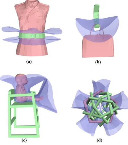
Fig. 1. Examples of the Interaction Bisector Surface (the blue surface) for two parts of the 3D scene (shown as red and green). (a) belt on uniform, (b) bag on hook, (c) baby on chair, (d) a pentagon tangled with other five pentagons
It is not an easy task to directly extend such an approach for 3D scenes where complex spatial relationships are present. Fisher and his colleagues encode the spatial context of 3D scenes using con-tacts between objects [Fisher et al. 2011] and the adjacency infor-mation represented by relative vectors [Fisher and Hanrahan 2010]. Although such approaches can successfully classify static scenes where objects are correlated only by simple adjacencies or support, they may not be enough for encoding more complex relations such as enclosures, links and tangles, or those that involve articulated models such as human bodies or deformable objects such as ropes and clothes. Therefore, a more descriptive representation that can evaluate the complex nature of interactions is needed for success-fully indexing such spatial relationships.
In this paper, we propose using the Interaction Bisector Surface (IBS), which is a subset of the Voronoi diagram, for the represen-tation of the spatial context of the scene. The Voronoi diagram has been applied in indexing and recognizing the relationships of pro-teins in the area of biology [Kim et al. 2006]. In a similar
ner to the Voronoi diagram, the IBS is the collection of points that are equidistant from at least two objects in the scene. The IBS can describe the topological and geometric nature of a spatial relation-ship. By computing a topological feature set called the Betti num-bers, we can detect relationships such as enclosures and windings, which characterize scenes such as a house surrounded by fences, a woman with a hand bag hanging on her arm, or an object contained in a box. The geometric nature of the relationships can be analysed using the shape of the IBS, the direction of its normal vectors, and the distance between the objects and the IBS. The computation of the IBS makes minimal assumptions about the forms of data input, which can be polygon meshes, skeletons or point-clouds, making it applicable to a wide range of existing data. In this paper, we aim to analyse spatial relationships only based on the topological and geometric features, thus avoiding object labels as used in [Fisher and Hanrahan 2010; Fisher et al. 2011].
Using the IBS as the interaction descriptor, we present the fol-lowing three applications:
Interaction ClassificationThe topological and geometric fea-tures of the IBS can be used for the classification of different spatial relationships.
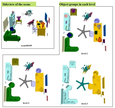
Automatic Construction of Scene Hierarchies Using scenes that are composed of multiple objects such as room data, we show that the IBS can be applied in composing a hierarchy that describes the scene. Given an input scene, we group individual objects or object groups iteratively using a closeness-metric based on the IBS. Content-based Relationship Retrieval Our distance function can be used for finding similar relationships in the database, based purely on the relationship information.
Contributions
—A rich representation of relationships between objects in a scene, which can encode not only the geometric but also the topological nature of the spatial relationships.
—An automated mechanism to build hierarchical structures for scenes based on the spatial relationships of the objects.
—Similarity metrics for object-object relations and an approach for conducting context-based relationship retrieval.
The rest of the paper is organized as follows. After reviewing re-lated work in Section 2, we explain how to compute the IBS in Sec-tion 3, and its topology and geometry features in SecSec-tion 4. Then we propose an algorithm of building hierarchical structures for 3D scenes in Section 5. Based on the hierarchy, we explain how to rep-resent and measure the similarity of spatial contexts of objects in Section 6. Next, we show the experimental results in Section 7 and finally discuss the methodology and draw conclusions in Section 8.
2. RELATED WORK
We will first review works about 3D analysis and synthesis, which is a relatively new topic in the area of computer graphics. As medial axis is quite relevant to the IBS, we also review works about medial axes computation, and discuss the difference between medial axis and the IBS.
Analysis of 3D Objects and Scenes Recently, research into re-trieval and synthesis of 3D objects and scenes is growing due to the large amount of datasets available from, for example, Google Warehouse. Among such works, we are mainly interested in meth-ods that use the spatial relationships between multiple components in the data to describe the entire object or scene.
Several methods to analyse the structure of man-made objects have been recently proposed [Wang et al. 2011; Kalogerakis et al. 2012; van Kaick et al. 2013a; Zheng et al. 2013]. Wang et al. [2011] compute hierarchical pyramids of single objects based on the sym-metry and contact information. Kalogerakis et al. [2012] produce a probabilistic model of the shape structure from examples. Van Kaick et al. [2013a] uses a co-hierarchical analysis to learn mod-els. Zheng et al. [2013] build a graph structure from an object based on the spatial relationships of the components. As these methods are focused on single objects, the spatial structure of the objects is mainly based on the contact information, and the spatial relation-ships between separate parts are either ignored or only described by simple features such as relative vectors. Some recent works which aims for shape matching [van Kaick et al. 2013b; Zheng et al. 2012], propose new features based on pairwise points to encode the spatial context of shapes. These works also show that the spa-tial relationship between different parts of a 3D shape is important for shape understanding.
Structure analysis is also applied for scenes composed of multi-ple objects. Fisher et al. [2011] propose to construct scene graphs based on contextual groups and contact information between ob-jects. The scenes are then compared by a kernel-based graph match-ing algorithm, which has been applied in image analysis [Har-chaoui and Bach 2007]. The spatial relationships are highly ab-stracted by simple binary information of contacts. Yu et al. [2011] encode the relationships between furniture using metrics such as distance, orientation and ergonomic measures. The objects are grouped into hierarchies to learn the furniture arrangements. The complex interactions are manually labelled by the users in these studies due to the difficulty of automatically learning them by sim-ple measures. Fisher et al. [2012] learn contexts from examsim-ples by using Bayesian networks and mixture models. The relationships be-tween adjacent objects are represented by relative vectors, and are compared using bipartite matching. Paraboschi et al. [2007] use the distance from the barycenter, height distance and geodesic distance as the metric and compose a graph Laplacian to encode the rela-tionship of adjacent objects. Tang et al. [2012] similarly encode the interactions of multiple characters by applying Delaunay tetra-hedralization to the joints composing the character skeletons and computing the Hamming distance between them. These methods require the objects to be manually labelled in order to reinforce the simple representations used to describe the relationships. In many situations, however, the objects may not be tagged or tagged in an inconsistent manner.
In our case, we compare scenes which may be composed of unla-belled, dense mesh structures that may interact with one another in a complex manner. Such relationships are difficult to represent us-ing simple relative vectors or distances. We cope with this problem by using a more expressive representation that takes into account the relationships of the entire surfaces of the objects composing the scenes.
Medial Axis and Shape Recognition Here, we briefly review the medial axis computation and application, and how the medial axis relate to our work.
a graph matching problem, for which various efficient techniques have been proposed.
The previous research for computing the medial axis can be clas-sified into two main categories: the continuous method and the dis-crete method. The continuous method [Culver et al. 1999; Sher-brooke et al. 1995], aims to compute an accurate medial axis for polyhedrons, while the discrete method [Amenta et al. 2001], ap-proximates the medial axis by sample points on the boundary of the shape.
One issue with using the medial axis for pattern recognition is its instability, as small perturbations of the boundary of the shape can introduce large changes to its medial axis. Many methods, in-cluding [Sud et al. 2007; Imai 1996], are proposed to get the stable subset of the medial axis which is not sensitive to small perturba-tions. Our method does not suffer from such instability as we only use the bisector surface that is defined between two groups of poly-gons. We shall discuss more about this in Section 3.
The medial axis can be computed inside an object as well as at the external area of the object. The bisector surface, which is a subset of the medial axis, has been applied in representing pro-tein interactions [Kim et al. 2006]. Instead of dealing with specific structures like proteins, we define a more general metric, which can compare the spatial relationship between interacting parts by mea-suring the features of the IBS. In our research, we use the IBS as a descriptor of the spatial relationships between objects in the scene.
3. INTERACTION BISECTOR SURFACE
Here we define the IBS and then describe how it is computed.
3.1 Definition
Given N point sets S1, S2, ...SN in the 3D space where Si = {pi
1, p
i
2, ..., p
i
ni}, an Interaction Bisector Surface(IBS) divides the
space into N regions with following properties:
—Points from the same point set lie in exactly one region. —If a pointq6∈ {S1∪S2∪...SN}lies in the same region asSi,
then the Hausdorff distance(in the Euclidean space) between set {q}andSiwill be shorter than the Hausdorff distance between set{q}andSj, whereSjis any other point set.
In other words, the IBS is the set of points equidistant from two sets of points sampled on different objects. It is an approximation of the Voronoi diagram for objects in the scene. Examples of the IBS for different scenes are shown as blue surfaces in Figure 1. It can be either open or closed. Although the IBS can reach infinity when it is open (the same as the Voronoi diagram), we truncate it by a bounding sphere (details are given in Section 3.2). Despite the possibility that the IBS can produce a complicated polyhedral complex, it tends to form smooth shapes with stable topology when computed from objects in daily life such as those presented in the paper.
3.2 IBS Computation
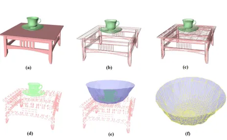
[image:4.612.318.550.76.219.2]Here we give details about how we compute the IBS for a given scene. We start by sampling points on the surfaces of the scene models uniformly, and then compute the Voronoi diagram for all these samples. The Quickhull algorithm [Barber et al. 1996] was used in this process. The result of the Quickhull algorithm is a sim-plicial complex consisting of polygons calledridges. Every ridge is equidistant to the two sample points which produce it. Hence there is a correspondence between ridges and the sample points. Assuming that the scene data is pre-segmented into objects, which
Fig. 2. Steps for computing IBS: Given a segmented scene (a) (in this ex-ample the scene have two segments: a cup and a table), which is composed of polygon meshes (b), we first subdivide the mesh to triangles of simi-lar size (c) and then take the centre points of each triangle (d). IBS is the Voronoi surfaces which produced by two samples from different objects (e) and is also represented by a polygon mesh (f).
Fig. 3. (a) Penetrations between the models and IBS, which is caused by the inadequate sampling on objects. (b) After after 4 iterations of refining processes, there is no penetration any more, and the shape of the IBS be-comes smoother (The big gap between the cup and the table is for visual-ization purpose.)
is usually the case in scene data, we only select ridges that corre-spond to sample points from two different objects for computing the IBS. These steps are shown in Figure 2.
As the IBS by definition could reach infinity, we trim it by adding a bounding sphere to the scene data to compute the Voronoi dia-gram. In practice, the bounding sphere is found in the following way. We first find the minimum bounding box of the scene, and use the centre of bounding box as the centre of the bounding sphere. The diameter of the sphere is set to 1.5 times the diagonal of the bounding box.
Special attention is needed if two objects are very close to each other, as there is a chance that the IBS will penetrate the objects due to the inadequate sampling density. In this case, we iteratively refine the IBS by the following process: if penetrations are found between the IBS and any object, we sample more on the parts of the object where the penetrations happen. Figure 3 shows the IBS between a table and a coffee cup. In this example, there are no more penetrations after four iterations.
[image:4.612.323.550.317.455.2]Fig. 4. The IBS (the blue line) is the stable part of the medial axis(the blue line and the grey lines). It does not fluctuate under subtle geometric changes.
Although the topological structure of the medial axis can be sen-sitive to subtle geometric changes of the relevant surfaces, the IBS is rather robust against such changes as it is computed between two objects. The instability of the medial axis is due to the “fluctuating spikes” [Attali et al. 2009], which are produced by concave dips on the surfaces (the grey branches in Figure 4). As the IBS is only produced between separate objects, such spikes are not included in its structure and therefore is less likely to be affected by subtle ge-ometric changes of the object. More examples of the IBS of of 3D object pairs are shown in Figure 1 and Figure 5.
Given a scene, we only need to compute the IBS for the whole scene once, and it already contains the spatial relation of every pair of objects. We denote the subset of the IBS between objectiand ob-jectjasIBS(i, j). Furthermore, a subset of the IBS between two groups of objects,gxandgy, can be represented byIBS(gx, gy)=
S
IBS(i, j)wherei∈gxandj∈gy.
4. IBS FEATURES
In this section, we give details about how to compute the topologi-cal and geometric features of the IBS.
4.1 Topological Features of the IBS
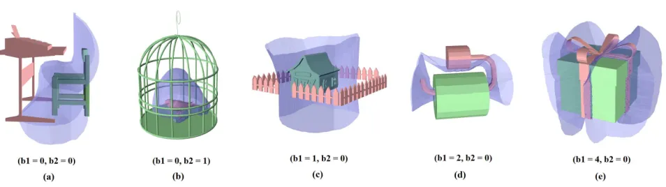
Topological descriptions of relationships are succinct and robust against small geometric variations. Consider a ball in a box. The description “in” here is irrelevant to the ball position or orientation as long as it is inside the box. Thus, capturing the topological nature of the interaction between two objects is crucial in relationship un-derstanding. A good indicator of the topological nature is the Betti numbers of the IBS. We will first briefly give the definition of Betti numbers and then demonstrate how it can be applied as a feature to classify complex interactions.
The Betti number is a concept in algebraic topology. Formally, the k-th Betti number refers to the number of independent k -dimensional surfaces [Carlsson 2009]. We make use of the sec-ond (denoted asb1) and third (denoted asb2) Betti numbers in
this research. They represent the number of two-dimensional or “circular” holes (b1), and the number of three-dimensional holes
or “voids” (b2). Intuitively speaking,b1 represents the number of
“cuts” needed to transform a shape into a flat sheet. For example, objects that are laterally surrounded by others, such as a house sur-rounded by fences (see Figure 5 (c)), forms an IBS of a cylindrical shape, resulting inb1 = 1. For objects tangled with other objects,
such as toilet paper (see Figure 5 (d)), a partial torus is generated, resulting inb1 = 2.b1 can be even larger under complex
inter-actions whose IBS involves a lot of loops (see Figure 5 (e)).b2
represents the number of closed surfaces. In our scenario, it counts how many objects are wrapped by other objects (see Figure 5 (b)).
The Betti numbers can be easily computed from the mesh data by the incremental algorithm [Delfinado and Edelsbrunner 1995].
4.2 Geometric Features of the IBS
Although the Betti numbers can distinguish the qualitative differ-ence of interactions, they cannot distinguish subtle differdiffer-ences. For example, the IBS of two boxes laterally adjacent to each other has exactly the same Betti numbers as that of an apple in a bowl. To ad-dress this problem, we evaluate the following geometric attributes of the IBS:
(1) geometric shape,
(2) distribution of the direction vectors, and
(3) distribution of distance between the IBS and the objects.
These features are computed at points sampled on the IBS. As different parts of the IBS are not equally descriptive of the rela-tionship, we use an importance-based sampling scheme that is de-scribed in Appendix A. In brief, more points are sampled where the IBS is in close proximity with the objects defining it.
Geometric Shape of the IBS The geometric shape of the IBS is useful for comparing the nature of the interactions. For example, when an object is simply parallel to another, the IBS will become planar, but it will form a bowl shape when one object is surrounded by another object.
Various shape descriptors can be considered for the IBS. One possibility is to use the curvature profile; however, the curvature data can be unstable as the IBS may include ridges with sharp turns. This occurs when the mapping of the closest point between the IBS and the object becomes discontinuous due to the concavity of the object. Also, the IBS may be either an open or closed surface.
Taking into account these characteristics, we use the Point Fea-ture Histogram (PFH) descriptor [Rusu et al. 2008a]; PFH is a his-togram of the relative rotation between each pair of normals in the whole point cloud. It describes the local geometrical properties by generalizing the mean curvature at every point. It provides an over-all pose and density invariant feature which is robust to noise. PFH is applied for 3D point cloud classification [Rusu et al. 2008a] and registration [Rusu et al. 2008b].
More specifically, for each sample point on a given IBS, we com-pute a 125-bin histogram of the relative rotation angles between the normal vector at the sample point and those of the other sample points. We produce a set of histograms for the whole IBS. Then we follow a method proposed in [Alexandre 2012]. We compute the centroid and the standard deviation for each dimension of the his-togram set, and use the resulting 250 dimension vector as the final feature of the IBS. More details for computing the PFH feature are described in Appendix B.
Direction The normal vectors of sample points on an IBS contain the direction information about the spatial relationship. For exam-ple, if all the normal vectors of the IBS are facing upwards, one of the object forming the IBS is above the other.
The direction of the IBS normal is defined so that it points toward the reference object. In our definition, spatial relations are unidirec-tional. The relationship of A with respect to B is different from B with respect to A. We first need to specify the reference object. As the IBS normal can be pointing either side of the IBS surface, we use the one that is defined on the side the reference object exists.
Fig. 5. The IBS (in blue) of two object scenes (a) table and chair, (b) bird in cage, (c) house surrounded by fences, (d) toilet paper on holder, (e) gift box and ribbon, and their Betti numbers.
respect to the reference object, we assume that the+zaxis of the scene is the vertical direction, and use the angle between the nor-mal vector and+z direction (denoted here byθ) to compute the direction feature. We computeθfor each sample on an IBS, and produce a uniform histogram with 10 bins in the range of 0 toπ. The number of samples which fall into each bin is counted, and normalized against the total number of samples.
Distance Between the Object Surface and IBS The distribution of the distance between the IBS and the object surface is descriptive about the relations of the two objects. The larger the distance is, the less likely that the two objects are closely related. We produce a uniform histogram with 10 bins whose range is between0to0.5×
d, wheredis the diagonal distance of the bounding box of the two objects. We compute the distance for each sample on the IBS, and accumulate the number of sample points that fall into each bin. The histogram is normalized by the total number of samples and is used as another geometric feature.
5. AUTOMATIC HIERARCHICAL SCENE ANALYSIS
In this section, we propose a method to automatically build a hier-archy out of a scene by making use of the IBS data. The method is an adapted version of the Hierarchical Agglomerative Clustering (HAC) algorithm [Hastie et al. 2009]. The resulting scene structure is used later for content-based relationship retrieval.
We first give the motivation, then a metric to measure inter-object and inter-group relations and finally an algorithm for constructing a hierarchy based on spatial relations.
5.1 Motivation
The idea to represent scenes by graph structures has been applied in content-based scene retrieval [Fisher and Hanrahan 2010; Fisher et al. 2011] and synthesis [Yu et al. 2011; Fisher et al. 2012]. In previous works, the relationships between objects in a 3D scene are either embedded at the design stage or computed based on con-tact [Fisher and Hanrahan 2010; Fisher et al. 2011; Yu et al. 2011]. Examples of such scene graphs are shown in Figure 6 (b)(d).
The major difference between our method and previous works is that we adopt a multiresolution structure that encodes not only the spatial relations of the individual objects but also those between the object groups, which are more descriptive about the scene, es-pecially when the number of scene components is large.
Fig. 6. Scene structures of two example scenes: scene-a and scene-b. (a) and (c) show the hierarchical structures produced by our method; (b) and (d) show the scene graph used in [Fisher et al. 2011].
Let us first describe the advantage of considering the inter-group relationship with an example. For the sake of simplicity, we shall call an object group acommunity. A community only containing an object and its immediately surrounding objects is called the lo-cal communityof the object. A larger community containing other objects further away in the scene is called theextended commu-nityof the object. In scene-b of Figure 6, the status of the bowl can be described through its local community (the table and the bowl) first, and then further described by the relation between the the bowl’s local community and other communities (the two chairs) in the room. This description is far easier to recognize than using the raw, low level relationships of all the individual objects, such
[image:6.612.322.550.277.536.2]as is done by Fisher et al. [2010; 2011] as shown in scene-c in Fig-ure 6. The reason behind this is that humans tend to recognize a scene at the group level when observing it from a global perspec-tive [Goldstein 2010], by aggregating objects based on proximity, continuation, uniformity, etc. Our multiresolution representation is also more descriptive than the raw graph description by Fisher et al.. This can be seen through scene-a and scene-b in Figure 6; the two are the same under the raw graph representation (Figure 6 (b) and (d)) while the objects are grouped based on the spatial rela-tionships and distinguished in our multiresolution representation (Figure 6 (a) and (c)).
The terms “local” and “extended” community are only used for description purpose, and we do not arbitrarily classify neighbours into such categories. The inter-community relationships are pro-duced by first grouping individual objects into communities of closer objects and then recursively grouping them into larger com-munities. The details of this procedure are described in Section 5.2. This structure naturally forms different abstraction levels of the scene. Given a reference object, the inter-community relationships on each level reflect the relationships between the reference object and the scene at different abstraction levels.
5.2 Closeness Measure and Hierarchy Construction
To formally define the hierarchy and the relationships between one object and its environment, we define a measure calledcloseness
between communities that can contain only an object or a set of ob-jects. Given a sceneSwithncommunities,S={g0, g1, ..., gn−1},
the closeness measure between any two communities,gxandgy, is defined as below:
Rc(gx, gy) =Rratio(gx, gy) +Rratio(gy, gx) (1)
Rratio(gx, gy) =
W IBS(gx, gy)
W IBS(gx,S \gx)
IBS(gx, gy) =
[
i∈gx,j∈gy
IBS(i, j) (2)
whereIBS(i, j)represents the IBS subset shared by objectiand
j. The functionWcomputes the weighting of the IBS region. Note that simply computing the area ofIBS(i, j)does not give a good measure of the importance as mentioned in Section 4.2. In prac-tice, we useW IBS(i, j)
=nwherenis the number of sample points (that is described in Section 4.2) on the IBS shared between objectiandjinstead of computing its actual area. This is to weigh more the parts where the two communities are closely interacting with each other.
Rratio(gx, gy)is thecommitmentofgxtowardsgy;Rratio(gx, gy) is larger ifgxshares a large amount of the IBS withgythan with other communities. It also meansgx commits more togythan to any other communities. Note thatRratio(gx, gy)is not necessarily symmetric. Essentially,Rcmeasures the relation between two com-munities under the context of the whole scene.
WithRcas a distance function, we present an adopted HAC al-gorithm to build a hierarchical structure of a scene. This hierarchy is built iteratively in a bottom-up fashion. Starting from individual objects (leaf nodes of the tree), we measure theRcbetween nodes and group them into nodes that represent bigger communities. A merge can combine more than two nodes. This process is repeated until the whole scene is merged into one big single node. The de-tails of the approach can be found in Algorithm 1. Figure 6 (a) and (c) show simple examples.
Data: A sceneG, grouping thresholdτ,0≤τ≤1
Result: A hierarchyH
Compute and sample IBS ; Initialize the first levelG0
={g1, g2, ...gm}; Initialize the current levelG=G0;
Define next levelG′={g′
1, g′2, ...g′n}; whilesize(G)>1do
AppendGtoH; n = size(G);
compute matrixM1n∗n:M1i,j←Rc(i, j)(Equation 1) ;
computeM2n∗n:
M2i,j←
1 ifgiandgjhave contact(s)
0 otherwise
for0≤i, j≤ndo ifM26=0then
M3i,j←M1i,j∗M2i,j;
else
M3i,j←M1i,j;
end
ifM3i,j> τthen
if∃g′, g′⊂G′, g
i⊂g′orgj⊂g′then ifgj6⊂g′,g′ ←g′ ∪gj,elseg′ ←g′ ∪gi; else
buildg′←g
i∪gjandG′←G′∪g′; end
end end
G←G′;
end
AppendGtoH;
Algorithm 1:Automatic Hierarchy Construction
6. SIMILARITY METRICS BASED ON IBS
In this section, we describe how we make use of the features of the IBS and the scene structure to compute the similarity of in-teractions. We first explain the similarity measure of relationships between two objects. We then describe the similarity measure of relationships between reference objects and their immediate neigh-bours in the local community. Finally, we explain the similarity measure of relationships between objects and their extended com-munities. Note that these measures are only used for content-based retrieval explained in Section 7.3. For classification, a different equation based on Radial Basis Function is used, which is ex-plained in Section 7.1.
6.1 Similarity Measure for Relationships Between Two Objects
Given two sets of IBS features,f1 andf2, we first use a simple
Kronecker delta kernel as a measure for the topological features:
δ(fb
1, f
b
2) =
1 iffb
1 =f2b
0 otherwise (3)
wherefb
i is the vector of the Betti numbers offi.
Next we define a measure for the geometric features of the IBS that uses theL1 distance of the PFH, direction and distance
fea-tures:
dgeo(f1, f2) =a·L1(f1PFH, f
PFH
2 ) +b·L1(f1dir, f
dir
2 )
+c·L1(f1dis, f
dis
wherea+b+c= 1 (0≤a, b, c≤1), fPFH
i ,fidir andfidis are the PFH, direction and distance features offirespectively. As the three features are in different ranges, we apply theInverse Variance Weighting scheme[Hartung et al. 2011] to theL1distance of three
features. We seta= 0.1,b= 0.4andc= 0.5in our experiments. We combine the topology and geometry measures of the IBS, and compute the final similarity between two IBS by:
ssr(fi, fj) =δ(fib, f b j)
w·(1−d
geo(fi, fj)) (5) wherewis a “switch” for using topological features. From the ex-periment in Section 7.1 we can see that Betti number is quite use-ful for complex interactions like tangles or enclosures, while it can contradict geometric features for data that contains penetrations. The metric function for measuring the similarity between two sets of IBS features should be defined based on the nature of the dataset and the purpose of retrieval. If the data mainly contains complex relations,wshould be 1 so that the Betti number is used as a fil-ter for different infil-teraction types with respect to its topology; if the data mainly contains simple relations, which have Betti numbers
b1 = 0, b2= 0,wshould be set to 0 to speed up the computation
and avoid the influence of possible penetrations.
6.2 Similarity Measure for Local Communities
We now describe how we can compare two objects with respect to their local communities. We define a profile of objectoiin a local communityg={o1, o2, ...om}by:
flocali= [
1≤j≤m,j6=i
fi,j; (6)
wherefi,jis the feature set computed from the IBS between object
iandj. Therefore,flocaliis the set of IBS features betweeniand all
the other objects ing. We callflocalithelocal profileofoi. Given
two objectsoi,o′
ifrom different communitiesgandg′, their local profilesflocaliandf
′
localiare first computed. Then we can compute
the similarity betweenoiando′iunder the contexts of their local communities. We define a similarity measureslocal, normalized in a way similar to the graph kernel normalization [Fisher et al. 2011]:
slocal(i, i′) =
K(i, i′)
max(K(i, i), K(i′, i′)) (7)
K(i, i′) =X
i∈g
X
i′∈g′
ssr(flocali, f ′
locali) (8)
wheressris defined in Equation 5.
6.3 Similarity Metric for Extended Neighborhood
After definingslocal, we are ready to combine it with the hierarchi-cal structure and define a profile for an objectoiat every level of the hierarchy. For a scene S and its hierarchy, we assume that the leaf nodes are at level 1. Letlddenote the nodes atdth level so thatldis a set of communities{gd1, g
d
2, ..., g
d
m}. Assume an object
oi∈gxd,1≤x≤m, a profile ofoiat thdth level is defined as:
fd exti=
[
1≤y≤m,y6=x
fgd
x,gdy (9)
wherefgd
x,gydis the IBS feature set computed fromIBS(g
d x, gyd), which is the IBS subset shared by communitygd
xandg
d
y. Then we can compute the similarity between objectsoi∈gdxando′i ∈g′x
d
from different scenes at the leveldby:
sextd(i, i′) =
Ke(i, i′)
max(Ke(i, i), Ke(i′, i′))
(10)
Ke(i, i′) =
X
i∈gx X
i′∈g′ x
ssr(fextdi, f
d ext′
i) (11)
wheredis the level.
Finally, given a search depth parameterddepth, we can find the similarity between objectoi ∈gxdando′i ∈gx′
d
by accumulating their similarities from level 1 toddepth:
sall(i, i′) = ddepth
X
d=1
γds extd(g
d k, g
d
i′); (12)
whereγis set to 0.5 taken to the power ofdat each level. This is the contextual similarity for two objects in the database up to a given level.
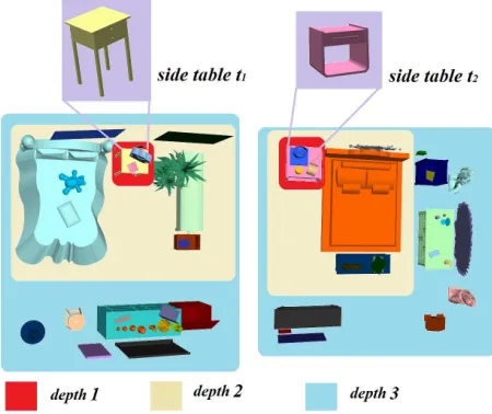
A detailed example can be found in Figure 7. Assume that we want to compare side tablet1 and side tablet2 in two scenes. If
ddepth = 1, then onlyslocal(t1, t2)is calculated. The only objects
involved are the objects on top oft1 andt2. Ifddepth = 2, then
sext1=slocal(t1, t2)andsext2(t1, t2)is calculated based on the IBS
subset between the red areas and other areas within level 2. Finally,
[image:8.612.326.551.369.558.2]sall(t1, t2)=sext1+0.5×sext2(t1, t2).
Fig. 7. An example of hierarchical comparison. The two side tables are the “centre” objects we want to compare. The red, yellow and light blue regions contain the side table’s neighbours in level 1(bottom level), level 2, and level 3 of the scene structures respectively.
7. EXPERIMENTS AND EVALUATIONS
In this section, we present three experiments. The first is super-vised classification of interactions between two objects, the second is building hierarchical structures for 3D scenes, and the third is relation-based retrieval. For each experiment, we first explain the idea, then give experimental settings and results, and present the evaluation at the end.
Table I. Descriptions of spatial relationships of 16 classes
Examples Description Examples Description 1, 2 Enclose 3, 4 Encircle
5 Interlocked 6 Side by side, similar sizes 7, 8 Tucked in 9, 10 Side by side,
one considerably higher 11, 12 Loosely above 13, 14 On top of 15, 16 Partially inside, with open areas
7.1 Classification of Interactions
Here we show how geometrical and topological features in different combinations help in classifying two-object relationships.
Experiment The data set we use contains 1381 items, each of which is an object pair. We ask the user to label them based on their spatial relations. The database consists of 16 classes. We show one example in each class in Figure 8. Descriptions for these classes are summarized in Table I.
In order to facilitate the description, we refer to the interactions with Betti numberb1 = 0, b2 = 0assimple relations, and
[image:9.612.54.291.405.625.2]com-plex relationsotherwise. The first part of our database contains 1289 items that are extracted from the Stanford Scene Database used in [Fisher et al. 2012]. Since this mainly consists of simple relations, we denote it asS. We ask the user to label the data into meaningful classes, which turn out to be 11 classes (class 6 to class 16 in Figure 8). The second part of the database contains 92 ex-amples of complex relations labelled into 5 classes (class 1 to 5 in Figure 8) by the user. As all data in this part represent complex relations, we refer to it asC.
Fig. 8. Examples from 16 classes in our database. One example for each class.
We do the experiments first on S and C individually and
then on the whole database S +C. In each experiment, the
data is split into a training set and a testing set in the ratio of 7:3. We performed classification on different combinations of features to investigate how individual features and combinations
of them influence the classification. Specifically, we test PFH (P), PFH+Direction (PDI), PFH+Direction+Distance (PDD) and PFH+Direction+Distance+Betti number (PDDB). The feature vec-tor in each experiment is a concatenation of the involved individual features. Individual features are first normalized. In different exper-iments, we use different combinations of the normalized features. In other words, if we use a fixed-length feature vector to repre-sent each feature with non-zero values on its corresponding dimen-sions and all other value zeroed, then the concatenation can also be seen as linearly summing up several features. We tried different weights for this linear combination to achieve good results. Empir-ically an equal weighting scheme is used for all the classification experiments. For comparison, we also tested two features: absolute height displacement and absolute radial separation used in [Fisher and Hanrahan 2010] for the whole data set, denoted by DIS.
We choose Support Vector Machines (SVMs) [Boser et al. 1992][Cortes and Vapnik 1995] for the classification task because of their simplicity. Specifically, we use the soft margin method [Cortes and Vapnik 1995]. For our multi-class problem, a one-v.s.-onescheme is used. For the kernel, we use a Radial Basis Function (RBF),K(x, y) =e−θkx−yk2
wherexandyare the concatenated feature vectors. To find the best parameter values, we do 5-fold cross-validation and hierarchical grid search. We start with coarser grids, then subdivide the best grid for another iteration of search un-til the improvement of the accuracy falls below 0.001 or it reaches the maximum iteration. Finally, we train the model with the whole training set again using the optimal values and then test it. For im-plementation, we use libSVM [Chang and Lin 2011].
Evaluation and Comparison The prediction accuracy is shown in Table II. The first column consists of the data set. The first row lists features. The cells are filled with prediction accuracies of each experiment. They are calculated by feeding the testing data set into the trained SVM classifier and the accuracy is the percentage of correctly classified data out of the whole testing data set.
Overall, IBS features are more discriminative for one-to-one re-lationship classification than DIS used in [Fisher and Hanrahan 2010]. Note that in the paper [Fisher and Hanrahan 2010] , they achieve good retrieval results by using other information such as labelling, but we aim to avoid using it as such data is not always available. The results shows that DIS does not perform as well as the IBS features under our setting.
For further comparison of features within PDDB, one can see that the PFH descriptor of the IBS already gives good results for this 16-class classification problem. On top of PFH, the direction improves the result. On the complex data set, the distance is a bit detrimental to the result. This is because distance and direction can contradict on another in this data set. However, we find that the pre-diction accuracy of the complex data set is also 100% when just us-ing PFH and Betti numbers. It reflects the fact that for complex rela-tionships, direction and distances are not discriminative enough. It also shows that Betti numbers provide vital information, especially in classifying complex interactions.
Table II. Prediction Accuracy
P PDI PDD PDDB DIS
S 78.33% 84.07% 85.90% 82.77% 41.25%
C 80.00% 96.00% 92.00% 100.00% 44.00%
S+C 76.47% 81.37% 83.33% 84.31% 38.73%
[image:10.612.322.548.101.314.2]Fig. 9. Confusion matrices of PDDB (Left) and DIS (Right) on the whole data set (16 classes). Results are normalized within each column.
Table III. Cross-validation accuracy and time consumption
PDDB DIS Cross-validation accuracy 83.56% 39.36% Time for cross-validation (secs) 580.56 106.07 Time for training (secs) 0.22 0.06
In Figure 9 we plot the confusion matrix. The values are normal-ized for each column. The classes that have the lowest prediction accuracies are class 9 and 10 (Figure 9 left). Most of their mis-classified instances are in class 6. Shown in Figure 8 and Table I, class 6, 9 and 10 all have a “side-by-side“ relation. But class 9 and 10 have one object higher than the other. The height difference in some scenes is not big enough to be classified correctly. This is the main source of the prediction error.
PerformanceTable III shows the timing and accuracy information of cross-validation and training on the whole data set (S+C). The first row contains best average accuracy of the 5-fold cross valida-tion during the hierarchical grid search. The second row contains the time consumption for the grid search and the last row contains the training time after we find the optimal values of the parameters.
The configuration of the computer where these numbers are cal-culated is: Intel i7-2760QM CPU, 8G memory, Windows 7 Profes-sional 64 bit and Matlab R2012a (64 bit).
7.2 Building Hierarchical Structures for 3d Scenes
Experiment We build hierarchical structures for 130 scenes in the Stanford Database by using Algorithm 1. One example of the re-sults is shown in Figure 10. More rere-sults are shown in the supple-mentary document.
The parameterτ controls the speed of merging when building the hierarchy. A lowerτ will merge more nodes together in each round, which means that the number of levels is smaller compared to the structure built with a higherτ. The choice ofτshould depend on the nature of the data as well as the higher-level application. For the Stanford Scene Database, we foundτ = 0.32gives visually reasonable structures for most of the scenes. The average number of levels of the hierarchical structure under thisτsetting is 2.89.
Fig. 10. An example of the hierarchical structure. The objects in the same group are shown in the same colour.
Evaluation and Analysis As the scene structure will be used as the input for content-based retrieval, the stability of the hierarchi-cal structure with respect to the parameter setting is important. We evaluate the stability of our HAC algorithm in this experiment, and its benefits for retrieval will be evaluated together with the retrieval results in the next section.
Following the scheme by Goodman and Kruskal [1954], which has been employed to compute the stability of hierarchical algo-rithms for image segmentation [MacDonald et al. 2006] and speech classification [Smith and Dubes 1980], we assess the stability of generating the hierarchical structure using a consistency measure (denoted here byγ) of how the merges happen under different pa-rameter settings. Briefly speaking,γ (−1 ≤ γ ≤ 1) is the dif-ference between the probability that the “correct” and the “wrong” order occurs. See Appendix C for the details of computingγ. In our algorithm, the grouping thresholdτis the main parameter. We check the stability of the structure under different values ofτ. For each scene, we compute five hierarchies by varyingτ from 0.1 to 0.5 with an interval of 0.1. Then, we compute theγfor every pair within the five hierarchies. Finally, we use the mean of theγ, de-noted here byˆγ, as the indicator of the stability of our method. We computeγˆfor 130 scenes, and the averageγˆis 0.989, with the low-est stability 0.779 (scene00042), which means the stability of our algorithm is very high.
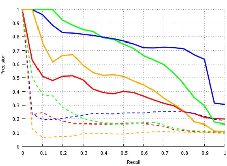
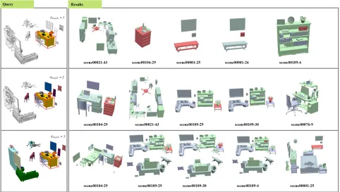
7.3 Content-based Retrieval
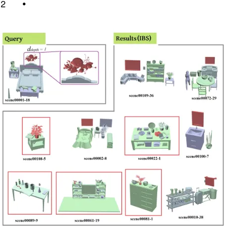
Experiment We tested the capability of our algorithm for content-based scene retrieval using a data set that consists of 130 scenes, which come from the Stanford Scene Database. We first calculate the hierarchical structures by the techniques explained in Section 5. The user then selects any single object from a scene as a query. Then the system returns objects in any scene which has similar spa-tial relations with their surrounding objects.
Fig. 11. The solid lines show the precision-recall curve for our algo-rithm on four test scenes. The dashed lines show the precision-recall curve when using the DIS feature. The Ids of the four queries in the Stanford Scene Database are: scene00050-object8(red), scene00118-object14(green), scene00109-object14(blue), scene00087-object37(yellow)
Fig. 12. Scene regions and precision-recall curves for differentddepths.
Each row corresponds to one query we used for the user study. The red object in the scene is the query object. The boundary lines in the left column show the regions correspondent to the p-r curves of the same colour.
Evaluation and Comparison The retrieval results of an exam-ple scene with different depthddepthare shown in Figure 14. Com-pared with the results in Figure 15 that use the displacement fea-tures (DIS) [Fisher and Hanrahan 2010], it can be observed that
our system returns much more contextually similar results. More retrieval results are presented in the supplementary document.
In order to evaluate our system, we prepared manually labelled data, which is produced as follows. Four query objects were se-lected from the Stanford Scene Database, and then for each query object an additional 500 objects are randomly selected from the database. The set of 500 objects were shown to the user with the scene in random order, and the user was asked if the object has similar spatial relations with the surrounding objects as compared to the corresponding query object. We label the spatial relations as similar if more then half of the users think they are similar. Ten users including students and staffs from different schools in the uni-versity took part in the user study.
For quantitative evaluation of the results, the precision and re-call curves (pr-curve) are drawn based on the search results and the ground-truth (manually labelled) data. In Figure 11, we present the curves based on our features (solid lines) and DIS (dashed lines). It can be observed that all the solid lines show significantly higher precision than the dashed lines of the same colour, which indicates that our features out-perform the DIS feature. Our algorithm returns 50% of similar results with a precision of at least 40%, meaning that at least 1 in every 2.5 resulting scenes is desirable.
We now show the results of analysing the extent of the com-munity (ddepth) the users take into account when comparing the similarity of relationships. Figure 12 shows the pr-curves for three query scenes with differentddepthvalues. In Figure 12 (a), the pr-curve forddepth= 1 gives slightly higher precision thanddepth= 2, which means that the users tend to pay more attention to the imme-diate neighbours of the “plate” (which are the toast, the table, and the other objects on the table) than those in the extended commu-nity. The results in Figure 12 (c) are similar to (a), but there is a larger difference in precision between the two depths. In Figure 12
(b),ddepth= 2 gives the highest precision, which means the users
also consider the objects in the extended communities when evalu-ating the similarity of the spatial relations. We can assume that fac-tors such as the scale of the scene and the density of objects affect the perception of the neighbourhood. The scene in Figure 12(b) has more objects densely located around the desk compared with the desk in Figure 12(c) and the scale is larger than the scene shown in Figure 12(a).
Figure 13 shows a failure case for our method on the Stanford Scene Database, with half of the top ten results (object on table) not matching the query object (decoration hang above the bed). As the bottom of the decoration is almost in contact with the bed head, it is similar to the “one object on another” examples in terms of spatial relationship. This can be a typical failure case of retrieval results not being consistent with the user’s intuition due to the fact that we do not take into account any geometry information of the individual objects nor their semantic labels. The failure cases are mostly removed from the retrieval results when the decoration is lifted a little bit so that the relationship between the decoration and the bed head are not misunderstood as contacts.
8. CONCLUSION AND DISCUSSIONS
[image:11.612.55.288.321.594.2]Fig. 14. Retrieval results by using IBS features. (left) In the query scene, the object with a bounding box (the desk) is the query object. We show the other objects within the search depth in colour while leaving the rest of the scene in grey. (right) The resulting scenes from left to right are in order of similarity. The red object is the retrieved object with a similar context to the desk. We also only render the objects within the search depth for the resulting scenes.
Fig. 15. Retrieval results by using the DIS feature.
[image:12.612.62.544.444.717.2]Fig. 13. Failure case. The results with red bounding box are not satisfac-tory, as they are “object on table” which the query is “object hanging above another object”.
and it provides a new perspective to model spatial relationships. In addition, we have proposed an automated mechanism to understand the structure of big scenes consisting of a large number of objects. Knowing the hierarchy of big scenes is crucial for applications such as content-based relationship retrieval. Because of the nature of the IBS, the calculation naturally rules out relationships between ob-jects that are too far from each other or have too many obob-jects in between. The structure of the IBS segments the scene into groups at every level. Therefore, we are able to automatically build up a hierarchical structure that has meaningful geographical groups. We also propose similarity metrics based on the IBS that effectively distinguish different types of spatial relationships between objects or object groups. These metrics are equipped with the scene hierar-chy so that comparison can be made between objects based on their contexts. Finally, we also show how the features, metrics and algo-rithms based on the IBS can be applied to solve practical problems. Although our approach to computing the IBS is a heuristic, it is a good compromise in terms of computational cost and precision. For the computation of the IBS, we use a sampling-based approach in which points are sampled on the object surfaces and then the Quickhull algorithm [Barber et al. 1996] is used. This is a heuristic approach that does not guarantee the exact topology and geometry of the resulting medial axis. This could be an issue if we need to match the homotopy of the IBS. In order to avoid such confusion, we use abstract topology features (the first and second Betti num-bers) whose values are less influenced by the accuracy of the IBS. Also, the geometric features of the IBS are statistical values that are less influenced by the accuracy of the IBS. In addition, exact methods to compute the medial axis [Culver et al. 1999] and bisec-tor surface [Elber and Kim 1997] are not practical to be applied in a set of high resolution meshes. In summary, our method makes use of features that are less computationally costly and less affected by parameter values.
Limitations Although the IBS is good for identifying spatial re-lationships, the computational cost is higher compared with other
simple features used in [Fisher and Hanrahan 2010]. We believe that it is a fair trade-off between precision and performance. The method can be easily parallelized, and can greatly benefit from implementing on multi-core systems. Secondly, the discriminative power of the IBS deteriorates when the distance between objects increases. When there are just two objects in the scene and they are far apart from each other, we suspect that IBS features can be replaced by simpler features used in [Fisher and Hanrahan 2010] such as the height displacement and radial separation. Lastly, as we focus on relationship understanding in this research, individual ge-ometry plays a less important role. This is different from previous works. Hence, for applications such as retrieval, it might cause con-fusion when the user tries to retrieve scenes not only with similar relationships but also with similar geometries.
Future Work We believe that the potential of using IBS for spa-tial relation representation has not been fully explored. In the fu-ture, one possible direction is to use it for comparing two scenes. This can be useful for whole scene retrieval. Another promising direction is to further exploit IBS features and explore along the time domain. By observing the feature variations on the time di-mension, we might be able to understand, recognize and classify animated scenes. At the same time, by adding human knowledge via learning algorithms, we can pursue a semantic understanding of the relationships between motions and environments.
REFERENCES
ALEXANDRE, L. A. 2012. 3D descriptors for object and category recog-nition: a comparative evaluation. InWorkshop on Color-Depth Camera Fusion in Robotics at the IEEE/RSJ International Conference on Intelli-gent Robots and Systems (IROS). Vilamoura, Portugal.
AMENTA, N., CHOI, S.,ANDKOLLURI, R. K. 2001. The power crust. In
Proceedings of the sixth ACM symposium on Solid modeling and appli-cations. 249266.
ATTALI, D., BOISSONNAT, J.-D.,ANDEDELSBRUNNER, H. 2009. Stabil-ity and computation of medial axes - a state-of-the-art report. In Mathe-matical Foundations of Scientific Visualization, Computer Graphics, and Massive Data Exploration, T. Mller, B. Hamann, and R. D. Russell, Eds. Mathematics and Visualization. Springer Berlin Heidelberg, 109–125. BARBER, C. B., DOBKIN, D. P.,ANDHUHDANPAA, H. 1996. The
quick-hull algorithm for convex quick-hulls. ACM TRANSACTIONS ON MATHE-MATICAL SOFTWARE 22,4, 469483.
BELONGIE, S., MALIK, J.,ANDPUZICHA, J. 2002. Shape matching and object recognition using shape contexts. IEEE Transactions on Pattern Analysis and Machine Intelligence 24,4, 509–522.
BOSER, B. E., GUYON, I. M.,ANDVAPNIK, V. N. 1992. A training algorithm for optimal margin classifiers. InProceedings of the 5th An-nual ACM Workshop on Computational Learning Theory. ACM Press, 144152.
CARLSSON, G. 2009. Topology and data.Bulletin of the American Math-ematical Society 46,2, 255–308.
CHANG, C.-C.ANDLIN, C.-J. 2011. LIBSVM: a library for support vec-tor machines. ACM Transactions on Intelligent Systems and Technol-ogy 2,3, 27:127:27. Software available at http://www.csie.ntu.edu.tw/ cjlin/libsvm.
CHANG, M.-C.ANDKIMIA, B. B. 2011. Measuring 3D shape similarity by graph-based matching of the medial scaffolds. Computer Vision and Image Understanding 115,5, 707720.
CULVER, T., KEYSER, J.,ANDMANOCHA, D. 1999. Accurate computa-tion of the medial axis of a polyhedron. InProceedings of the fifth ACM symposium on Solid modeling and applications. 179190.
DELFINADO, C. J. A.ANDEDELSBRUNNER, H. 1995. An incremen-tal algorithm for betti numbers of simplicial complexes on the 3-sphere.
Computer Aided Geometric Design 12,7 (Nov.), 771–784.
ELBER, G.ANDKIM, M.-S. 1997. The bisector surface of freeform ratio-nal space curves. InProceedings of the thirteenth annual symposium on Computational geometry. ACM, 473–474.
FISHER, M.ANDHANRAHAN, P. 2010. Context-based search for 3D mod-els.ACM Transactions on Graphics (TOG) 29,6, 182.
FISHER, M., RITCHIE, D., SAVVA, M., FUNKHOUSER, T.,ANDHANRA
-HAN, P. 2012. Example-based synthesis of 3D object arrangements. In
ACM SIGGRAPH Asia 2012 papers. SIGGRAPH Asia ’12.
FISHER, M., SAVVA, M., ANDHANRAHAN, P. 2011. Characterizing structural relationships in scenes using graph kernels. ACM Trans. Graph. 30,4.
GIANNAROU, S.ANDSTATHAKI, T. 2007. Object identification in com-plex scenes using shape context descriptors and multi-stage clustering. In
2007 15th International Conference on Digital Signal Processing. 244– 247.
GOLDSTEIN, E. B. 2010.Sensation and perception. CengageBrain. com. GOODMAN, L. A.ANDKRUSKAL, W. H. 1954. Measures of association
for cross classifications.Journal of the American Statistical Association, 732764.
HARCHAOUI, Z.ANDBACH, F. 2007. Image classification with segmen-tation graph kernels. InIn Proc. CVPR.
HARTUNG, J., KNAPP, G.,ANDSINHA, B. K. 2011. Statistical meta-analysis with applications. Vol. 738. Wiley. com.
HASTIE, T., TIBSHIRANI, R.,ANDFRIEDMAN, J. 2009.Elements of Sta-tistical Learning. Springer My Copy UK.
IMAI, T. 1996. A topology oriented algorithm for the voronoi diagram of polygons. InProceedings of the 8th Canadian Conference on Computa-tional Geometry. Carleton University Press, 107–112.
KALOGERAKIS, E., CHAUDHURI, S., KOLLER, D., ANDKOLTUN, V. 2012. A probabilistic model for component-based shape synthesis.ACM Trans. Graph. 31,4, 55.
KIM, C.-M., WON, C. I., CHO, Y., KIM, D., LEE, S., BHAK, J.,AND
KIM, D.-S. 2006. Interaction interfaces in proteins via the voronoi dia-gram of atoms.Computer-Aided Design 38.
MACDONALD, D., LANG, J.,ANDMCALLISTER, M. 2006. Evaluation of colour image segmentation hierarchies. InProceedings of the The 3rd Canadian Conference on Computer and Robot Vision. 27.
PARABOSCHI, L., BIASOTTI, S.,ANDFALCIDIENO, B. 2007. Comparing sets of 3D digital shapes through topological structures. InGraph-Based Representations in Pattern Recognition, F. Escolano and M. Vento, Eds. Number 4538 in Lecture Notes in Computer Science. Springer Berlin Heidelberg, 114–125.
RABINOVICH, A., VEDALDI, A., GALLEGUILLOS, C., WIEWIORA, E.,
ANDBELONGIE, S. 2007. Objects in context.ICCV.
RUSU, R., MARTON, Z., BLODOW, N.,ANDBEETZ, M. 2008a. Learn-ing informative point classes for the acquisition of object model maps. In10th International Conference on Control, Automation, Robotics and Vision, 2008. ICARCV 2008. 643–650.
RUSU, R. B., MARTON, Z. C., BLODOW, N.,ANDBEETZ, M. 2008b. Persistent point feature histograms for 3D point clouds.
SEBASTIAN, T. B., KLEIN, P. N.,ANDKIMIA, B. B. 2001. Recognition of shapes by editing shock graphs. InICCV. 755762.
SHERBROOKE, E. C., PATRIKALAKIS, N. M.,ANDBRISSON, E. 1995. Computation of the medial axis transform of 3-d polyhedra. In
Proceed-ings of the third ACM symposium on Solid modeling and applications. 187200.
SMITH, S. P.ANDDUBES, R. 1980. Stability of a hierarchical clustering.
Pattern Recognition 12,3, 177187.
SUD, A., FOSKEY, M.,ANDMANOCHA, D. 2007. Homotopy-preserving medial axis simplification. International Journal of Computational Ge-ometry & Applications 17,05, 423451.
TANG, J. K. T., CHAN, J. C. P., LEUNG, H.,ANDKOMURA, T. 2012. Retrieval of interactions by abstraction of spacetime relationships. Com-puter Graphics Forum 31,2.
VANKAICK, O., XU, K., ZHANG, H., WANG, Y., SUN, S., SHAMIR, A.,
ANDCOHEN-OR, D. 2013. Co-hierarchical analysis of shape structures.
ACM Trans. Graph. 32,4, 69.
VANKAICK, O., ZHANG, H.,ANDHAMARNEH, G. 2013. Bilateral maps for partial matching. InComputer Graphics Forum. Wiley Online Li-brary.
WANG, Y., XU, K., LI, J., ZHANG, H., SHAMIR, A., LIU, L., CHENG, Z.-Q.,ANDXIONG, Y. 2011. Symmetry hierarchy of man-made objects.
Computer Graphics Forum 30,2, 287–296.
YU, L.-F., YEUNG, S.-K., TANG, C.-K., TERZOPOULOS, D., CHAN, T. F.,ANDOSHER, S. J. 2011. Make it home: automatic optimization of furniture arrangement.ACM Trans. Graph. 30,4 (July), 86:186:12. ZHENG, Y., COHEN-OR, D.,ANDMITRA, N. J. 2013. Smart variations:
Functional substructures for part compatibility. Computer Graphics Fo-rum (Eurographics) 32,2pt2, 195–204.
ZHENG, Y., TAI, C., ZHANG, E.,ANDXU, P. 2012. Pairwise harmonics for shape analysis.
APPENDIX
[image:14.612.321.547.456.560.2]A. SAMPLING
Fig. 16. (left) The direction angle of a polygon on the IBS, (right) The sampling result
Here we describe how we sample points on the IBS where we compute the geometric features. This is done by calculating the weights of the triangles composing the IBS. First, we define a direc-tion angleαfor each triangle. A triangle T on the IBS is equidistant to sample points,sbandscono1ando2respectively. Let us define
a vector,v, from the center of T tosband a normalnof T pointing towards the side ofo1.α(Figure 16(a)) is the angle betweenvand
n. Note that this angle is the same if we compute it between T and
o2because the normal is flipped in that case. The larger the angle
is, the higher the chance that the sample point is far away from the
Fig. 17. PFH angles
objects defining it and less informative about the interaction. We compute a weightW(T):
W(T) =Warea(T)∗Wscene-distance(T)∗Wangle(T) (13)
whereWarea(T)is the area of triangle T andWangleis computed as:
Wangle=
1− α
45◦ ifα <45◦
0 otherwise (14)
Wscene-distanceis computed by:
Wscene-distance= (1−
d D)
n
(15)
dis the distance between the center of T andsa (orsb).D =
ddiag/2whereddiag is the length of the diagonal of the bounding box of the whole scene. We empirically setnequal to 20. We then normalized W(T) for all the triangles. Next, we set up a target num-ber for all triangles and the final target numnum-ber for each triangle is the target number times the triangle’s weight. Finally, we use the final target numbers to do random sampling on every triangle. Fig-ure 16(b) shows the result of the weighted sampling.
B. POINT FEATURE HISTOGRAM (PFH)
PFH is a feature for encoding the geometry of a point cloud. Given two points(Figure 17),p1 andp2, with normalsn1 andn2, three
unit vectors (u,vandw) are built by the following procedure: 1)u
is the normal vector ofp1, 2)v=u× p2−dp1, 3)w=u×v.d=
kp2−p1k2Then the difference betweenn1andn2are represented
by three angles(α, θ, φ)which are computed as:α=v·n2,φ=
u· p2−p1
d ,θ =arctan(w·n2, u·n2). The triplet< α, φ, θ >
is computed for each pair of points in the k-neighbourhood, and are binned into a histogram. Usually each angle is divided intob
equal parts, and the triplet can form ab3
size histogram in which each bin represents a unit combination of the value ranges for each value. In our case, we compute the triplet for each pair of points in the point cloud which is a set of samples computed by using the method described previously. We setb= 5. So the PFH feature we use is a 125-length vector.
C. STABILITY
Here we explain the definition ofγ introduced by Goodman and Kruskal [Goodman and Kruskal 1954]. Consider two hierarchical structures for the same data,h1andh2, and two pairs of elements of
this datapi= (xi1, xi2)andpj= (xj1, xj2). The rankr(h, p)is
defined as the level at which the two elements of pairpfirst appear in the same cluster in hierarchyh. Over all the pairs of elements in
the data, set
Πs=
Pr{(r(h1, pi)< r(h1, pj)∧r(h2, pi)< r(h2, pj))∨
(r(h1, pi)> r(h1, pj)∧r(h2, pi)> r(h2, pj))}
Πs=
Pr{(r(h1, pi)< r(h1, pj)∧r(h2, pi)> r(h2, pj))∨
(r(h1, pi)> r(h1, pj)∧r(h2, pi)< r(h2, pj))}
Πt=
Pr{(r(h1, pi) =r(h1, pj))∨(r(h1, pi) =r(h1, pj))} (16)
Then
γ= Πs−Πd 1−Πt
(17)
γmeasures the difference between the probabilities of “right
or-der” and “wrong oror-der”. In other wordsγshows how much more