Using Bayesian dynamical systems, model averaging and neural networks to determine interactions between socio-economic indicators

Using Bayesian dynamical systems, model

averaging and neural networks to determine

interactions between socio-economic

indicators

Bjo¨ rn R. H. Blomqvist1*, Richard P. Mann2, David J. T. Sumpter1

1 Uppsala University, Department of Mathematics, Uppsala, Sweden, 2 University of Leeds, School of Mathematics, Leeds, United Kingdom

*[email protected]

Abstract

Social and economic systems produce complex and nonlinear relationships in the indicator variables that describe them. We present a Bayesian methodology to analyze the dynamical relationships between indicator variables by identifying the nonlinear functions that best describe their interactions. We search for the ‘best’ explicit functions by fitting data using Bayesian linear regression on a vast number of models and then comparing their Bayes fac-tors. The model with the highest Bayes factor, having the best trade-off between explanatory power and interpretability, is chosen as the ‘best’ model. To be able to compare a vast num-ber of models, we use conjugate priors, resulting in fast computation times. We check the robustness of our approach by comparison with more prediction oriented approaches such as model averaging and neural networks. Our modelling approach is illustrated using the classical example of how democracy and economic growth relate to each other. We find that the best dynamical model for democracy suggests that long term democratic increase is only possible if the economic situation gets better. No robust model explaining economic development using these two variables was found.

1 Introduction

In recent years, an extensive amount of data describing the state of social and economic sys-tems has become available. For example, the World Bank collects statistics on global develop-ment data since 1960, and has made them freely available in the form of indicator variables of education, health, income, but also pollution, science and technology, government and policy performances [1]. Data availability has opened up possibilities for a vast number of studies on evolution of the political, economical and sociological aspects of global development. Some examples include: causes of economic growth [2]; impact of democracy on health, schooling and development [3,4]; globalization and changes in societal values [5]; and relationships between liberalism, post-materialism and freedom [6]. Studies of social systems often consider different scales—e.g. community, municipality, states, and countries,— but address a common

a1111111111 a1111111111 a1111111111 a1111111111 a1111111111

OPEN ACCESS

Citation: Blomqvist BRH, Mann RP, Sumpter DJT

(2018) Using Bayesian dynamical systems, model averaging and neural networks to determine interactions between socio-economic indicators. PLoS ONE 13(5): e0196355.https://doi.org/ 10.1371/journal.pone.0196355

Editor: Bryan C Daniels, Arizona State University &

Santa Fe Institute, UNITED STATES

Received: October 12, 2017

Accepted: April 11, 2018

Published: May 9, 2018

Copyright:©2018 Blomqvist et al. This is an open access article distributed under the terms of the

Creative Commons Attribution License, which permits unrestricted use, distribution, and reproduction in any medium, provided the original author and source are credited.

Data Availability Statement: Data for GDP per

capita is available from The World Bank (World Development Indicators) & Democracy index from Welzel C. (2013). Freedom rising: Human empowerment and the contemporary quest for emancipation. Cambridge University Press.

Funding: The author(s) received no specific

funding for this work.

Competing interests: The authors have declared

fundamental question: is it possible to extract the underlying essential relationships and devel-opment patterns of indicator variables from time series data [7]? Knowing such relationships would constitute a significative step towards interpreting, predicting and possibly controlling, social and economical development.

Linear and non-linear interactions between indicator variables are common in social sys-tems [8–10], but time series data are often noisy and incomplete, posing significant challenges in the identification of such fundamental relationships.

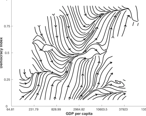
Let us take as an example the extensively studied, and hotly debated, relationship between democracy (D) and economic development (G) measured as GDP per capita [11–15]. In our study, time series data forDis based on the Freedom House political rights and civil liberties scores [16–18], weighted by the human-rights-performance, taking values between zero and one. The World Bank provides time series data ofGin U.S. dollar and in total we include data for 174 countries from 1981 and 2006, for a total of 3445 data points, averaging 19 data points per country. The dynamic relationship underlying these data can be conveniently repre-sented as a vector field in the (D,G) state space, as shown inFig 1. We obtain this visual

Fig 1. Naive approximation of the non-linear dynamics relationship between democracy (D) and log GDP per capita (G). The average change of all

data points in theGandDdirections is calculated in the state space of 100 equally sized regions visualized using an interpolating stream-slice plot. Where there are no lines, there is no data available.

representation by computing the change of all data points in theGandDdirections, we then divide the state space into 100 equally sized regions (10 by 10), average the changes in the data points within each area, and finally visualize the resulting vectors using an interpolating stream-slice plot. Although this is a naive approximation,Fig 1provides a picture of the non-linear nature of the democracy-GDP relationship.

It still remains unclear how much of the observed pattern inFig 1is due to a genuine rela-tionship between the indicators and how much is random noise in data. Such aspect as non-linearity and noise in the data significantly lowers the accuracy of the equation-based statistical models that one would traditionally use to fit data.

Within the fast-growing field of machine learning, artificial neural networks (ANN) are a simple, useful and accurate tool for modeling non-linear and complex systems, even when the available data is noisy [19–21]. Based on nonparametric estimations, this method can serve as a universal approximator [22], enabling fitting of data without constraints and guidance from theory, and is widely used in forecasting, modeling and classification. Since the 1990s, neural networks have been applied in fields as diverse as medical diagnosis [23], forecasting ground-water levels [24], speech recognition [25,26], and species determination in biology [27]. Recently, the nonlinearities characterizing social-economical systems have lead researchers in this area to turn to machine learning techniques [28]. Models obtained with ANN and similar prediction-oriented methods accurately reproduce empirical patterns. However results from ANNs essentially remain black boxes [29], making it difficult to translate from a fitted model to insights into the relationships between indicators.

Recently, Ranganthan et al. [15] introduced an approach to analyze time series data of social indicators that starts to bridge the gap between black-box machine learning algorithms and traditional statistical models by finding coupling functions [30] of the dynamical socio-eco-nomics interactions. Coupling functions are used for studying dynamics in many applications, such as: chemistry [31–33]; cardiorespiratory physiology [34,35]; neural science [36]; commu-nications [37]; and social science [3,15,38–41]. Ranganthan et al. [15] developed a Bayesian algorithm to trade-off between high explanatory power and complexity when selecting the best polynomial model to fit data. With this approach they were able to identify non-linear, dynam-ical relationships between indicator variables. In particular, when studying the relationship between democracy and economic development they found the best function to describe changes in democracy to be

dD

dt ¼0:11G 3

0:067D

G: ð1Þ

According to this expression, democracy increases once GDP per capita has reached a certain threshold that depends on the democracy level itself. The best model for GDP per capita was

dG

dt ¼0:014þ0:0064DG 0:02G; ð2Þ

telling us that most of the change in GDP would be explained by a positive constant which is decreased in richer but less democratic countries. Their approach has been extended to prob-lems with more than two variables, and used to analyze human development [15,42,43], the environment [44], democracy [3] and school segregation [40].

this number was limited to one model per number of terms in model), and to significantly speed up computational time. Furthermore, the novel aspect of assessing all potential models allows us to rank them and to discuss the relative importance and robustness of different linear and non-linear terms and their combinations by studying how often they recur. On the other hand, we compare our improved approach, i.e. the (1) Bayesian-selected ‘best model’, with two other approaches for modelling time series in social economical systems, i.e. (2) model averag-ing (over a subset of models obtained with our Bayesian approach) and (3) artificial neural net-works. Our ultimate aim is to select the best models distinguishing genuine relationships between indicator variables from random noise, retaining prediction estimates and in the meantime the highest explanatory power.

The paper is structured as follows. In the methods section (2) we describe the general framework we use to represent time series data (2.1), and the three approaches we consider to fit these data: our improved Bayesian-selected best model (2.2), Bayesian model averaging (2.3) and neural networks (2.4). In section 3 we report the results obtained by applying these three approaches on a case study, the relationship between democracy and GDP per capita. In section 4 we compare our Bayesian best model approach to the other two, discuss pros and cons, and compare our results on democracy and GDP with other studies.

2 Methods

2.1 Representation of time series data

We assume the social systems we investigate are described bynindicator variables, as democ-racy and GDP per capita in the example above (wheren= 2). Each individual entitymin this system, e.g. a country, a state, a city, provides a discrete time series for each indicator variable

xi(t),i2[1, 2,. . .,n] during a time periodT. Here, we interpret these individual time series as

realizations of paths of the same global system, but starting from different initial conditions. In other words, by this we mean that we assume that all entities within the investigated social sys-tem is governed by the same dynamical relations between indicator variables and their individ-ual time series are stochastically realizations of the dynamics staring from different initial conditions. This corresponds with discarding the individual, possibly large, differences between entities, assuming their evolution is affected only by their position in the indicators state space (x1,x2,. . .,xn). These assumptions enable us to fit the individual time series to

obtain a global model for the dynamical changes in the indicator variables. In particular, we aim at giving an accurate estimate of global indicators’ changes between timetandt+ 1 depending only on their value at timet, i.e. on their position in the state space.

2.2 Bayesian best model

The Bayesian ‘best model’ selection we propose here fits time series data for the indicator vari-ables to a model constituted by a system ofnordinary differential equations

dx1

dt ¼ f1ðx1;x2; :::;xnÞ þ1 dx2

dt ¼ f2ðx1;x2; :::;xnÞ þ2

.. .

dx_n

dt ¼ fnðx1;x2; :::;xnÞ þn:

Here,f1,. . .,fnare unknown coupling functions of the indicator variables and we assume

uncorrelated random noise termsi. The selection process takes the three following steps: (1)

Define all the possible model configurations; (2) fit the data to these configurations through Bayesian regression; and (3) compare model configurations and choose the best suitable model. Notice that although for notation convenience we write these equations in continuous time, we actually fit difference equations as available data is often reported at discrete times.

Step 1: Possible model configurations. To enhance interpretability, we choose to approx-imate the functionsfiwith polynomials consisting of linear and non-linear combinations of

the indicator variables. Typically, we use terms up to order three and define a model configura-tionM_ias any subset of the coefficients of such combination. Including a considerable amount of non-linear terms allows for multi-stable states which are frequently found in social systems [15,45]. For example, in a model withn= 2 our preliminary choice of functions is:

fðx1;x2Þ ¼ a0þ a1 1þx1

þ a2 1þx2

þa3x1þa4x2

þ a5 ð1þx1Þð1þx2Þ

þa6 x1 1þx2

þa7 x2 1þx1

þa8x1x2þa9x 2 1þa10x

2 2þ

a11 ð1þx1Þ

2

þ a12 ð1þx2Þ

2þa13x 3 1þa14x

3 2þ

a15 ð1þx1Þ

3

þ a16 ð1þx2Þ

3

;

ð4Þ

and a model configurationM_iwould be any subset of the coefficients {a0,. . .,a16} for a total

of 217= 131,072 configurations. This choice follows [15], but we have rescaled the variables to take values between zero and one and included a +1 in terms with denominators to avoid sin-gularities. The chosen functional form offioffers the highest degree of flexibility for systems

with relatively smalln, but it may be adjusted by adding or removing terms. We have tested our Bayesian framework on normalized input variables, in a setup without variables in denom-inators. The resulting ‘best models’ provided similar dynamics, but we argue our proposed model configurations are better for interpretation.

Step 2: Fit data to model configurations. In this step we obtain the coefficient values by applying Bayesian linear regression [46,47] on all the possible model configurations. The Bayesian linear regression practically consists in (1) assigning prior distributions to the unknown coefficients in each configuration; (2) Get the likelihood of the coefficients given the data; (3) Determine the posterior distribution of the coefficients by combining the priors and the likelihood using Bayes theorem [47].

In standard linear regression, one fitsnresponse variables y =x(t+ 1)−x(t) to the explana-tory variables X. The explanaexplana-tory variablesXis an×pdesign matrix consisting of linear and nonlinear terms in the tested model configurationM_i, wherenis the number of observations and p is the number of terms in the tested model configuration. The model for the response variable is typically divided into two components, deterministic and gaussian noise:

y¼Xbþ ð5Þ

A common way of finding an approximation of the unknown slope coefficientsb2Rp_is

finding maximum likelihood estimates^b_MLEthrough [47]:

^

bMLE¼ ðX T_XÞ 1

XT_{y: ð6Þ}

In principle, by evaluating the log-likelihood, i.e. the logarithm of the probability of observ-ing the data given model parameters of modelM_i, we could find the model that best repre-sents data. The likelihood in our setting is [46]

PðyjX;b;s2_{Þ ¼NðXb;s}2_{IÞ ð7Þ}

whereσ2is the regression variance. However, by definition the likelihood increases with the number of terms in the model, which would give us overcomplicated and difficult to interpret equations.

Our approach faces this problem by using a Bayesian approach and assigning prior distri-butionsp(β,σ2) on the coefficientsβandσ2. The priors are assigned only on the coefficients of the assumed prior model configurations, later after all of the data is presented, the model coef-ficients are updated. Since we introduce all of the available data at the same time, the priors are used once in our modelling approach and are assumed to be the same for all the different enti-ties (countries in our case) since they are assumed to be different realisations of the same social system. Combining prior knowledge and the likelihood of the data using Bayes theorem gives us the posterior distribution of coefficients [46]:

pðb;s2_{jy;XÞ ¼}PðyjX;b;s

2_Þpðb;s2_Þ

pðyjXÞ : ð8Þ

A flat prior distributionp(β,σ2) would give us the maximum likelihood estimate (6), assum-ing that the MLE lies within the range of the prior. This approach was for example used in [15]: in their implementation, they first found the model configurations with the highest log likelihood and then numerically calculated the marginal likelihood using Monte Carlo tech-niques for those models.

Here, we use a Normal Inverse Gamma (NIG) distributed prior with parameters (m0,V0, a0,b0):

pðb;s2_{Þ ¼ NIGðm}

0;V0;a0;b0Þ

¼ b

a0

0s

2ðaþðk=2Þþ1Þ

ð2pÞk=2jV0j 1=2

Gða0Þ

exp 2b0 ðb m0Þ

0

V 1

0 ðb m0Þ 2s2

ð9Þ

This choice has the double advantage of adjusting the punishment of overcomplicated models (more about this later) and, since it is a conjugate prior, of allowing for closed form cal-culations. Indeed, combining the likelihood with the NIG prior gives a NIG posterior distribu-tion with updated parameters (m, V,a,b) [46],

m ¼ ðV0þX

T_XÞ 1

ðV0m0þX

T_yÞ

V ¼ V0þX

T_X

a ¼ a0þn=2

b ¼ b0þ 1 2ðm

T

0V0m0þy

T_{y m}T

VmÞ:

ð10Þ

The best coefficientsβandσ2would then be given by the posterior mean,^b¼m

respec-tivelys2_¼ b

a 1fora

A similar but simpler choice for the prior which is commonly used is the Zellner g-prior [48], specified by

m0 ¼ 0

V0 ¼

1 gðX

T_XÞ

a0 ! 0

b0 ! 0

ð11Þ

This prior features convenient choices of the hyper-parameters, hence utilizing fewer parameters by lettingaandbgoing to zero, but retains the same essential features of the NIG prior. The parameters are set to be very small, but can’t be set to zero because this would brake downEq (15).

We choose the data dependent unit information priorg= "number of data points" [49], which effectively provides the same amount of information as one observation: the^b_MLEhas precision (XTX)−1/σ2and can be interpreted as the amount of information contained inn

observations. The unit information prior is then (XTX)−1/(nσ2), i.e. “one-nth” of the precision [50]. By using the sameg-prior for all model configurationsM_iwe therefore punish all over-complicated configurations in the same way. Moreover, this choice ofgalso puts more weight on the data and less on the prior when there is a lot of data available.

Another possible assumption on the prior distribution is to put the covariances of the expla-nation variables to zero,

m0 ¼ 0

V0 ¼ diag

1 gX

T_X

I

a0 ! 0

b0 ! 0

ð12Þ

where I is the identity matrix. This makes the prior behave like in ridge regression, by adding small values, inversely proportional to the variance of each explanation variable, on the diago-nal entities ofXTX. This choice of prior penalizes the least efficient parameters i.e. explanation variables with the most variance the most, and overcome ill-conditioned problems by punish-ing model configurations with collinearities. This assumption is motivated since we potentially use highly collinear explanation variables in some of the model configurations

e.g. 1

ð1þx1Þþ

1

ð1þx1Þ2þ

1

ð1þx1Þ3which can cause highly unstable estimations

^

b[51]. Since we are looking for models with high explanatory power, collinear terms are especially unwanted, since they do not add to the understanding i.e. we want simple models without two terms describing similar behavior.

The posterior mean of the coefficientβthen becomes

^

b ¼ ðXT_Xþdiag 1

gX

T_X

IÞ 1ðXT_{yÞ: ð13Þ}

Notice that asg! 1,^btends to the maximum log likelihood estimate. Conversely,g!0 would force the posterior towards the prior distribution making the inference impossible.

Step 3: Comparing model configurations. Once we fit each model configurationM_ito the same dataset by using the sameg-prior, we compare them by using their marginal likeli-hood to punish over complicated models, i.e those with many terms, by taking account for the uncertainty in the model parameters. The marginal likelihoodpðy;XjM_iÞ, is a measure of the probability of observing the data under the hypothesis that the model configurationM_iis true. This probability, also referred to as the model evidence [52], is calculated by integrating over the parameters in the model:

pðy;XjM_iÞ ¼

Z Z

pðy;Xjb_i;s2 Þpðb;s2

Þdb_ids2

ð14Þ

In our conjugate setting this integral can be computed analytically and the marginal likeli-hood forM_iis [46]:

pðy;XjM_iÞ ¼ 1 ð2pÞn=2

ffiffiffiffiffiffiffiffi

jVi

0j jVi

j s b a0 0 b a

GðaÞ

Gða0Þ

: ð15Þ

The intuition behind how the marginal likelihood punishes over-complicated models is the following; when the model complexity goes up, we spread out the prior over more terms and thereby have to perform integration over both ‘good’ and ‘bad’ terms, resulting in lower prior mass on the ‘good’ terms resulting in a lowered marginal likelihood. The marginal likelihood is also affected by ourgparameter.

To compare two configurationsM_iandM_jwe use the Bayes factor. The Bayes factor is the posterior odds divided by the prior odds, which is equal to the quotent of the marginal likeli-hoods (Eq 15):

BFðM_i;M_jÞ ¼jV

j

0j1=2jVi

j

1=2 ðbj

Þ

a

jVi

0j 1=2

jVjj

1=2 ðbi

Þ

a: ð16Þ

The higher the Bayes factor, the better the modelM_iis compared toM_j. In our study we compare all model configurations to the constant change modelM_consti.e. constant change between timestandt+ 1. By comparing all models to this benchmark model we can rank all possible models.

Additionally, we perform a visual comparison by plotting the dynamical changes in the phase space as described by each configuration, and compare the coefficient of determination (R2) of different model configurations. TheR2value gives us the proportion of the total varia-tion in the data picked up by our models. TheR2value is computed by

R2_¼1

P

iðfi yÞ

2

P

iðyi yÞ

2: ð17Þ

whereyis the mean change andyiis data points. Therefore a higherR2value corresponds to a

2.3 Bayesian model averaging

Bayesian model averaging weights the obtained model configurations by their marginal likeli-hood and combines them into an ‘average’ model [53,54]. This process integrates information from different models, providing a way of handling uncertainty and reducing the risk of overes-timation [53,55–57]. In this way, the uncertainty in model selection is treated in the same way as parameter uncertainty within a single model. In what follows we will compare the perfor-mances of three Bayesian average models obtained by combining the 1%, 10%, and 50% of the highest marginal likelihood configurations obtained with the process described in section 2.2.

2.4 Artificial neural network

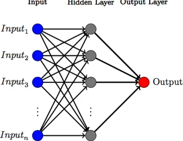
We use the Matlab neural network packagefitnet[58] to get a nonparametric estimate of the dynamical evolution of indicators that we can use as a benchmark to compare our Bayesian approach.fitnetis a feedforward neural network using a tan-sigmoid transfer function and a linear transfer function in the output layer [58]. In this paper, we choose to use one single hid-den layer and to vary the number of neurons to adjust for the level of fit of the network (see Fig 2).

In order to find a suitable number of neurons, not underestimating nor overestimating the network, we perform K-fold cross validation [59]. We use five folds and find the meanR2 val-ues for 1000 neural networks using 1-10 neurons (for each of the five folds). It is worth

Fig 2. Diagram of an feed-forward neural network with one hidden layer. This figure shows a generic feed forward

neural network with one hidden layer. The neural network usesninput variables and produce one output variable after passing through the network.

pointing out that since we assumed Gaussian noise above, theR2is related directly to likeli-hood of the model. The neural network model with the best cross-validated number of neu-rons (highestR2) is called the ‘best neuron network model’. After a suitable number of neurons is chosen, we train the neural networks using 70% of the available data, and then vali-dating and testing the model using 15% respectively. We compare our ‘best’ neural network model with two additional neural networks, namely one neural network model using only one neuron, representing an underestimating model and a model using ten neurons representing an overestimated model.

2.5 Surrogate data testing

To test the validity of the coupling functions we used surrogate data testing [60–62]. We gener-ate surroggener-ate data using the best model configurations of each coupling function and use boot-strapped initial data from the original dataset. The validity of the model from the original data is strengthen if we can reproduce the models generated from the surrogate data and thereby provide evidence that it was not just created by chance.

Specifically, the initial surrogate data is generated for 248 (number of countries and other sub-regions in the original data sets, including those regions without any data) countries using random sampling from our original data with replacement. We then apply the coupling func-tions i.e. best explicit funcfunc-tions, with corresponding noise terms, to simulate the changes the investigated indicator variables, producing data for an additional data 25 time-steps.

3 Results: Democracy vs. log GDP per capita

We now apply the three approaches to the same case study: the relationship between democ-racy (D) and log GDP per capita (G). Formally, the relationship betweenDandGtakes the form of two coupled differential equations:

dD

dt ¼ fDðD;GÞ þD

dG

dt ¼ fGðD;GÞ þG

ð18Þ

Firstly, we are interested in testing each approach for extracting the dynamical features of the coupled change in Democracy and log GDP per capita, i.e. the best fit offDandfGto the time

series data. We focus on the selection of the best functional form forfDandfGthrough our

Bayesian best model approach. Secondly, we cross-compare the performances of the three approaches and we analyze the recurrence of single and combined terms in the functionsfD

andfGextracted by the Bayesian best model. This allows us to assess the robustness of our

approach and to see to what extent it trades-off between accuracy and interpretability.

3.1 Best fit Bayesian models

We start from the generaln= 2 model described byEq (4). The model configurations are defined by subsets of the coefficients [a0,. . .,a16]. All possible combinations of these

coeffi-cients would give a total of 217model configurations. For simplicity and interpretability, we will restrict our analysis to model configurations with a maximum of 5 terms, for a total of P5

k¼1 17

k

¼9;401investigated configurationsM.

The best 1 to 5 term modelsMfor democracyfD(D,G) and log GDP per capitafG(D,G)

Bayes factor (Eq 16) with respect to a constant modelM_C, and to the coefficient of determina-tionR2(Eq 17).

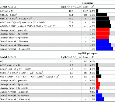
Except for the one-term model, all models for democracy include both democracy and log GDP per capita. The one-term model depends only onD, indicating that democracy typically grows with a rate that slows down as democracy itself increases. The best two-terms model can be rewritten in the formD(0.18G− 0.15D) suggesting a threshold atD= 1.2G. WhenD>1.2G

democracy decreases and whenD<1.2Gdemocracy increases. The best model for the change in democracy has three terms

fDðD;GÞ ¼0:16DG 0:14D

2_þ 0:01

ð1þDÞ3; ð19Þ

which is a combination of the one-terms and the two-terms models. In particular, the two first terms 0.16DG− 0.14D2indicate the existence of a threshold atD= 1.14Gas in the two-term model, but with updated coefficients. The four- and five-term models have a larger Bayes fac-tor than the one- and two-term models, but are not as good as the three-term model,

Table 1. Comparison of best models for democracy and log GDP per capita. The main three groups of rows

corre-spond to the three tested approaches, each shaded sub-row correcorre-sponds to the best model for the correcorre-sponding approach. For the Bayesian best model, columns display (left to right): the top 1-5 terms models, their log Bayes factor (BF), their configuration ranking (out of 9401), andR2_{value. We report the}

R2_{values for the average models and} feed-forward Neural Network models.

Democracy

Model:fD(D,G) logðBFðM;MconstÞÞ Rank R

2

0.013/(1 +D)3 _{12.6 8397 0.7%}

0.18DG− 0.15D2 47.4 251 3.0%

0.16DG− 0.14D2+ 0.01/(1 +D)3 54.0 1 3.6%

0.34D− 0.5D/(1 +G) + 0.03/(1 +G)3

− 0.09D3 _{52.9 4 3.9%}

0.2DG− 0.09D/(1 +G)− 0.05G3_{+ 0.02/(1 +}

D)2

− 0.1D3 _{50.3 41 4.0%}

Average model (1 procent) - - 3.8%

Average model (10 procent) - - 3.8%

Average model (50 procent) - - 3.5%

Neural Network (1 Neuron) - - 3.6%

Neural Network (4 Neurons) - - 4.1%

Neural Network (10 Neurons) - - 4.7%

log GDP per capita

Model:fG(D,G) logðBFðM;MconstÞÞ Rank R

2

0.011 0.0 360 0.0%

0.02D+ 0.01/(1 +D)3 8.2 1 0.7%

0.06D2_{+ 0.01/(1 +}

D)3

− 0.05D3 _{4.8 21 0.9%}

0.0005G3_{+ 0.06}

D2_{+ 0.01/(1 +}

D)3

− 0.05D3 _{0.6 248 0.9%}

0.35 + 0.01D/(1 +G)− 1.5/(1 +G)2− 0.14G2+ 1.21/(1 +G)3 0.3 279 1.5%

Average model (1 procent) - - 0.7%

Average model (10 procent) - - 1.0%

Average model (50 procent) - - 0.9%

Neural Network (1 Neuron) - - 0.5%

Neural Network (6 Neurons) - - 1.8%

Neural Network (10 Neurons) - - 2.2%

indicating that our approach successfully trades-off between accuracy and complexity in fitting this indicator.

For the log GDP per capita, the best model with only one term gives a constant rate of eco-nomic growth of 1.1% per year. Model configurations with two and three terms depend only on democracy, while models with four and five terms include both democracy and log GDP per capita. In terms of Bayes factor, the best model has two terms

fGðD;GÞ ¼ 0:008Dþ

0:005

ð1þDÞ3: ð20Þ

This model suggests that a potential driver of change in log GDP per capita is democracy. The first term indicates that log GDP per capita increases when democracy increases. The sec-ond term is also positive but gives a bigger contribution when democracy levels are low. As a result, GDP grows slowest whenD= 0.116, a level corresponding to rather undemocratic countries such as Burundi, Dominican Republic, Hungary in 1981, or Angola and Guinea in 2006. AsDincreases past this level the economy grows more rapidly.

3.2 Comparison of the three methods

Overall, our approach identifies two best models for democracy and GDP both featuring a rel-atively low amount of terms, which would make them easy to interpret. However, while the measures for the goodness of fit data are high in the case of democracy, this is not the case for GDP. This might indicate our modelling approach is not suitable for describing GDP data. Therefore, we first compare our best model to the fits given by the Bayesian average model and the neural network, and then investigate how often certain terms appear in the best 100 models extracted with our Bayesian approach.

The simplest way of comparing the three considered approaches is through the coefficient of determinationR2(seeTable 1). Our Bayesian best model for democracy has aR2of 3.6%, the best model obtained by model averaging is obtained by including the 10% top configura-tions and has aR2of 3.8%. The best neural network model (four neurons) gives the best fit for the democracy dataset, with aR2of 4.1%, but does not provide equations that we can easily interpret. Interestingly, theR2value of our Bayesian best model is very close to theR2of the best neural network, supporting the claim that our Bayesian best model is close to the best pos-sible fit to the given data set, with the additional advantage that it provides an explicit form for

fD. In the table we also include neural network models with one and ten neurons for

compari-son with to an under-, respectively over-trained neural networks.

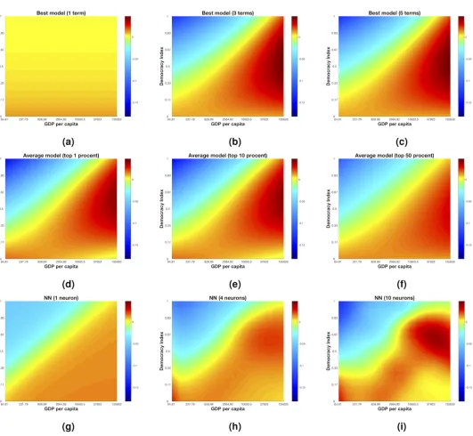
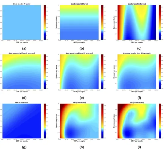
We can visualize our models using two dimensional heat maps. InFig 3(a)–3(c)we plot the best one-, three- and five-terms models respectively for democracy. A visual comparison of the three- (Eq 19) and five-terms models shows that the extra complexity of the latter does not sig-nificantly change the predicted dynamics. The average models (shown inFig 3(d)–3(f)) show a similar dynamics to the Bayesian best model. The non-parametric neural network models in Fig 3(g)–3(i)also show a similar behavior. The consistency of the pattern found in the change in democracy using these three different approaches suggests that, even though theR2are rela-tively small, these models reflect a genuine relationship between democracy and GDP over the past 30 years.

model. Moreover, the best one-term model for log GDP per capita is the 1.1% constant change model and is ranked 360 out of 9401 models. This high rank of the constant change model tells us that even the simplest model, not including democracy nor GDP per capita, is deemed to be almost as good as our ‘best model’, thereby weakening our belief in our model of GDP per capita.

A visual comparison of the Bayesian best model for log GDP (Fig 4b) with models with less and more terms (Fig 4a and 4c), with the average models (Fig 4(d)–4(f)), and with neural

Fig 3. Change in democracy (D). The three top figures in black (Fig 3 a,b,c) are visualizations of the changes in democracy for best models with one (Fig 3 a), three (Fig 3

b) and five (Fig 3 c) terms. The three figures in the vertical middle (Fig 3 d,e,f) represents 1% (Fig 3 d), 10% (Fig 3 e) and 50% model averaging models. The three figures at the bottom is representations of feedforward neural networks with 1 (Fig 3 g), 4 (Fig 3 h) and 10 (Fig 3 i) neurons in the hidden layer.

network models (Fig 4(g)–4(i)) reveals significant differences between models found with dif-ferent approaches. The average models are similar to the Bayesian best model, featuring a slightly more complex dynamics. The best (6 neurons) neural network model shows similari-ties with the 5-term Bayesian best model, but not with the highest-ranked two-terms model. Taken together, these results question the validity and reliability ofEq (20)as a model for the change of GDP per capita.

Fig 4. Change in log GDP per capita (G). The three top figures (Fig 4 a,b,c) are visualizations of the changes inGper capita for best models with one (Fig 4 a), two (Fig 4 b) and five (Fig 4 c) terms. The three figures in the vertical middle (Fig 4 d,e,f) represents 1% (Fig 4 d), 10% (Fig 4 e) and 50% model averaging models. The three figures at the bottom is representations of feedforward neural networks with 1 (Fig 4 g), 6 (Fig 4 h) and 10 (Fig 4 i) neurons in the hidden layer.

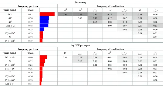
Finally, we test the robustness of our Bayesian best models by comparing all 9401 possible one- to five-term configurations. We argue that terms that appear repeatedly in different highly-ranked models are more likely to be a robust description of the data. InTable 2we report the eight most frequent terms among the top ranked 100 model configurations for both democracy and log GDP per capita. The frequency of two-terms combinations are also pre-sented, showing how likely it is for two particular terms to appear together. If two terms appear together frequently then we infer that this combination of terms is more robust.

For democracy, the termsDGand−D2, appear in both the best two-term and three-term models, and are the two most frequent terms among the 100 configurations with highest Bayes factor. We use 100 configuration to test if the terms are robust for the*1% of tested models to see if the terms in the best models are present still when we look beyond only the best mod-els. The termDGis involved in 82% of these models. Half of these models include the term −D2, while the other half include the term−D3. These two self-limiting terms,−D2and−D3, never appear together in the same model and clearly play the same role in fitting the data. This recurrence supports our belief that the democracy model extracted within our approach cap-tures a genuine aspect of the relationship between democracy and GDP.

The third term inEq (19), 1/(1 +D)3, does not appear as frequently and does not have as big impact on the change in democracy as the other two terms. This seems to suggest that the most robust description of the relationship between the rate of change of democracy and

Table 2. Robustness of terms for democracy (D) and log GDP per capita (G). The three columns furthest to the left shows the most eight most frequently recurring

terms among the top 100 models for (D) and (G). The columns to the right of show how often the terms appear in combination to each other. Red bars means a positive sign on the term and blue bars negative.

Democracy

Frequency per term Frequency of combination

Term model Procent −D2

−D3 D

ð1þGÞ −D

1

ð1þDÞ3 D

1

ð1þDÞ2

DG 0.82 0.41 0.41 0.30 0.25 0.17 0.18 0.00

−D2 0.50 0.00 0.30 0.17 0.07 0.09 0.08

−D3

0.49 0.17 0.08 0.12 0.05 0.08

−D/(1 +G) 0.48 0.00 0.07 0.09 0.17

−D 0.25 0.04 0.06 0.00

1/(1 +D)3 0.19 0.04 0.02

D 0.19 0.01

1/(1 +D)2 _0.17

log GDP per capita

Frequency per term Frequency of combination

Term model Procent D 1

ð1þDÞ3 ð1þGDÞ D

2 1

ð1þDÞ2

1

ð1þGÞ3

1

ð1þDÞ

D/(1 +G) 0.40 0.00 0.11 0.08 0.01 0.08 0.03 0.04

D 0.32 0.10 0.06 0.00 0.06 0.06 0.03

1/(1 +D)3 _{0.23 0.02 0.03 0.00 0.01 0.00}

G/(1 +D) 0.16 0.02 0.02 0.03 0.01

D2 0.16 0.02 0.03 0.02

1/(1 +D)2 0.16 0.01 0.00

1/(1 +G)3 _{0.13 0.00}

1/(1 +D) 0.11

GDP is

dD

dt Dð0:18G 0:15DÞ: ð21Þ

Although this model differs from the best model inEq (19), this functional form combines highestR2value, highest model ranking, robust combination of terms, and highest interpret-ability, which makes it the most explanatory and robust model for democracy.

For log GDP per capita (Eq 20), the termsDand 1/(1 +D)3are found in only the 32% and 23% of the 100 top-ranked configurations. The most frequent term,D/(1 +G), is found in 40% of the top 100 configurations. There are few consistent pairings of terms among the top 100 models, i.e.Dtogether with 1/(1 +D)3(10%) andD/(1 +G) with 1/(1 +D)3(11%), while the other combinations are evenly distributed. This seems to further indicate that the best model for log GDP per capita is not reliable in describing the available data.

Our chosen best models for democracy and log GDP per capita are stable with respect to reasonable changes in the g-prior’s parameterg. In particular, our approach returns the same ‘best models’ for bothD(Eq 19) andG(Eq 20), which are found atg= 3445, but with changed configurations’ ranking. For example, by doublingg(g= 2× 3445 = 7890) complicated models get punished more harshly and are thereby ranked lower. Halvingg(g= 3445/2 = 1722.5) also gives us the same ‘best models’, but complicated models are less punished. Instead, we obtain significantly different models when the parameterggets very large (g= 10100) or very small (g<300). In these extreme cases, the Bayesian selection favors respectively the one-term model presented inTable 1, and models with many terms, even though these terms are not consistent with our best one- to five-term models inTable 1.

3.3 Surrogate data testing

Even the best model for the changes in democracy (Eq 19) explains only a small part of the dynamics. A way to further investigate how robustly we can detect such a weak signal in noisy data is using surrogate data. We generated surrogate data usingEq (21)for the changes in democracy andEq (20)for changes in log GDP per capita. The surrogate data is generated with the same number of initial countries and time steps as in the original data and all other parameters are chosen to be consistent with the methodology presented in section 2.2. We sampled the initial values for the surrogate data set from the initial values in the original data. We use noise terms derived directly from empirical data (s2

D¼0:08,s

2

G¼0:02).

Even though we used a two term model (Eq 21) to generate data for democracy to fit the model we found that the following four term model, from the first fitting of surrogate data, was a typical best model for democracy,

dD

dt ¼0:186DG 0:154D 2

þ 0:208 ð1þDÞ3

0:181

ð1þDÞ2: ð22Þ

The fact that the resulting model is very similar, albeit with extra terms, provides additional evidence that our method is robust in the presence of noise. There were, however, additional spurious terms in the best models which may help us better understand our results. In particu-lar, it is interesting to note, that the term 1/(1 +D)3inEq (22)also arose in the overall best model (Eq 19). This strengthens our belief that our final model (i.e.Eq 21) for the dynamics in democracy is more parsimonious than a model including 1/(1 +D)3. It is plausible that these two latter terms is simply an artifact arising from our choice of prior i.e., the parametergis set to small (see the discussion in the end of section 3.2), rather than a genuine statistical

We also performed inference on the 1000 best model found for changes in democracy, using 1000 different sets of surrogate data. We found that the most frequent best model (609 out of 1000) was,

dD

dt DG D

3_þ 1 ð1þDÞ3

1

ð1þDÞ2; ð23Þ

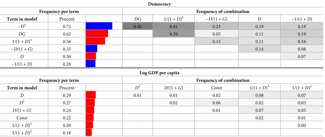
Note that we get the same model as inEq (22), with the difference thatD2is exchanged withD3.Table 3shows the frequency of occurrence of the different terms, and how often these terms are found in the same model configuration within the top 100 models, for all 1000 surro-gate data sets, for both democracy and log GDP per capita. For democracy, the best explicit models and the most frequent top configurations were found to be robust—with just small dif-ferences in coefficient values. The fact that the termsD2is exchanged withD3—note thatD2

andD3is very similar whenD2[0, 1], withD3is picked more frequently thenD2together withDGin models with more terms— indicates that the terms should be interpreted in quali-tative terms, rather than in terms of their specific exponents.

For log GDP per capita, the best models changed a lot for every realization. The termDand 1/(1 +D)3shows up as the most frequent and the fifth most frequent terms inTable 3. How-ever, the distribution of the top terms is very flat, indicating that the terms show up relatively equally among the best models. This further supports our previous conclusion that change in GDP can not be reliably modeled by democracy.

4 Discussion

In this paper, we accomplish two main goals. First, we improve upon the approach proposed in [15] by fitting data to equation-based ‘best models’ through Bayesian linear regression. Sec-ond, we develop a way of testing the robustness of the obtained models by comparing our

Table 3. Robustness of terms (surrogate data) for democracy (D) and log GDP per capita (G). The three columns furthest to the left shows the most eight most

fre-quently recurring terms among the top 100 models for (D) and (G) for 1000 generated surrogate data sets. The columns to the right of show how often the terms appear in combination to each other. Red bars means a positive sign on the term and blue bars negative.

Democracy

Frequency per term Frequency of combination

Term in model Procent DG 1/(1 +D)3 −D/(1 +G) D −1/(1 +D)

−D3 _{0.75 0.50 0.41 0.23 0.19 0.19}

DG 0.62 0.39 0.05 0.11 0.19

1/(1 +D)3 0.56 0.15 0.11 0.16

−D/(1 +G) 0.35 0.14 0.08

D 0.30 0.07

−1/(1 +D) 0.28

Log GDP per capita

Frequency per term Frequency of combination

Term in model Procent D2

D/(1 +G) Const 1/(1 +D)3 _{1/(1 +}

D)2

D 0.29 0.01 0.01 0.02 0.08 0.07

D2 0.27 0.02 0.06 0.02 0.03

D/(1 +G) 0.24 0.01 0.07 0.05

Const 0.22 0.02 0.01

1/(1 +D)3 _{0.20 0.00}

1/(1 +D)2 0.18

method with two prediction-oriented methods: model averaging and neural networks. We dis-cuss these two points in turn.

The strength of the approach developed in [15] is that it provides relationships between the variables, log GDP and Democracy in this case. They chose a two-term model (Eq 1) as the best model for democracy. Interestingly, their model displays the same threshold behavior as our best model for democracy (Eq 19). OurFig 3has clear similarities with the heat map of change in democracy presented in Fig 3a in [15] for all three modelling methods used in our paper. So even though we find different explicit expressions for the change in democracy, the overall dynamics is similar. The only visual difference is that our model gives a higher value for democracy, where the change is zero, for the low GDP per capita region. However, the terms selected are not the same as in our model. The primary reason for this difference is because we use more data: 174 countries instead of 74, and rescaled the indicator variables. Moreover, although being a convenient way of fitting equation-based ‘best models’ to data, their use of uniform flat priors makes analytical calculations not attainable for the posterior distributions. For this reason, they had to turn to numerical estimations, which caused loss of information and prevented them from studying and comparing all possible models, to check the robustness of the terms chosen. Furthermore, we argue that our final expressionEq (21)is not only checked for robustness (Table 2), it is also easier to interpret than the final expression in [15]. For these reasons, we argue that our model is a better description of the dynamics of democracy and log GDP per capita.

In our approach, we use Bayesian linear regression and a mathematically convenient prior [46,48]. This choice allows us to get closed form expressions for the marginal likelihoods and to significantly lower the computational burden. As a result, we can quickly compare and rank all model configurations, and study the frequency of single and combined terms in different models, thus performing an accurate analysis of the robustness of our ‘best model’.

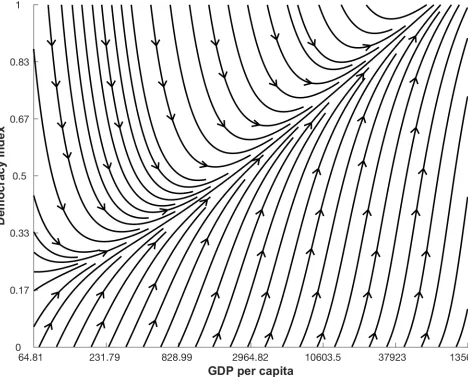
Social systems often display nonlinear interactions between indicator variables [8–10], making their study an interesting challenge. For example,Fig 1shows a clearly nonlinear rela-tion between democracy (D) and log GDP per capita (G). Here, we had the general goal of modelling this relation by distinguishing genuine interactions from noise.Fig 5shows the best relationship between democracy and log GDP per capita we can extract by applying our meth-odology. According to this plot, and thus our methodology, once noise is filtered outDandG

are connected by a simple threshold relationship. Moreover, we can extend our estimates of the dynamics in areas of the state space (D,G) where we have no data measured.

Our method relies on us comparing our explanation-oriented model with more predictive-oriented alternatives such as artificial neural networks. Artificial neural networks can be seen as universal estimators [22] and are widely used to study nonlinear systems appearing in social-economical systems [28]. Here we used ANNs as a benchmark to assess if the tradeoff between interpretability and predictive power is satisfactory. In our example of democracy and GDP per capita we found our modelling approach to give satisfactory results for democracy, but we also concluded the best model for GDP per capita was insufficient. We also used a Bayesian model-averaging approach as benchmark to account for model uncertainties in our ‘best models’.

overall negative and positive feedbacks captured by (Eq 19) are a robust feature of the data. Despite the lowR2of around 4% we have captured the underlying relationships. In contrast, when we subjected the GDP model (which hasR2of around 1%) to the same battery of tests, it repeatedly failed to give robust results. The techniques we have presented here, thus provide a way of interrogating and increasing our confidence in a model, even when it provides very weak explanatory power in a statistical sense.

A question that always arises in study like the one about the choice of priors. We choose to mimic a non-informative prior by setting the shape and rate parameters to be very small. This choice is common, and used for example in [63], but we have to be careful when using these choices when performing inference, since it can be sensitive to the small values, as implied in [64]. In our application, we can not see any problems regarding this, but users of our method-ology should be aware of these potential complications.

Fig 5. Relation between democracy and GDP per capita. Dynamics of the relation between democracy (D) and (G), in USD, using best models,Eq (19)

(D) andEq (20)(G), displayed using linear interpolated streamline plot.

Having benchmarks of neural networks and model averages to compare an equation-based model with is especially important if we wish to move up in dimensionality i.e. when studying multivariate coupling functions arising when studying systems with more than two indicator variables [65,66]. Adding variables into our social system makes them harder to visualize using two-dimensional heat maps, as we did in Figs3and4. With three-variables models we could visualize the relations between indicators and compare models using three-dimensional plots, but if we want to go even further up in dimensionality [3,42] we might need to assume that some variables are held constant—assuming that there are interactional terms to these additional variables. This would make the global relations harder to study. Providing explicit equation-based models and a way to test their robustness, our Bayesian-based approach is a valuable tool for understanding the relationships underlying complex social systems.

Author Contributions

Conceptualization: Bjo¨rn R. H. Blomqvist, Richard P. Mann, David J. T. Sumpter.

Formal analysis: Bjo¨rn R. H. Blomqvist.

Methodology: Bjo¨rn R. H. Blomqvist, Richard P. Mann, David J. T. Sumpter.

Software: Bjo¨rn R. H. Blomqvist.

Writing – original draft: Bjo¨rn R. H. Blomqvist, Richard P. Mann, David J. T. Sumpter.

Writing – review & editing: Bjo¨rn R. H. Blomqvist, Richard P. Mann, David J. T. Sumpter.

References

1. The World Bank, World Development Indicators;. Available from:http://data.worldbank.org[cited 5.10.2017].

2. Durlauf SN, Johnson PA, Temple JR. Growth econometrics. Handbook of economic growth. 2005; 1:555–677.

3. Spaiser V, Ranganathan S, Mann RP, Sumpter DJ. The dynamics of democracy, development and cul-tural values. PloS one. 2014; 9(6):e97856.https://doi.org/10.1371/journal.pone.0097856PMID: 24905920

4. Lindenfors P, Jansson F, Sandberg M. The cultural evolution of democracy: Saltational changes in a political regime landscape. Plos One. 2011; 6(11):e28270.https://doi.org/10.1371/journal.pone. 0028270PMID:22140565

5. Inglehart R. Globalization and postmodern values. Washington Quarterly. 2000; 23(1):215–228.https:// doi.org/10.1162/016366000560665

6. Welzel C, Inglehart R. Liberalism, postmaterialism, and the growth of freedom. International Review of Sociology. 2005; 15(1):81–108.https://doi.org/10.1080/03906700500038579

7. Opp KD. Modeling micro-macro relationships: Problems and solutions. The Journal of Mathematical Sociology. 2011; 35(1-3):209–234.https://doi.org/10.1080/0022250X.2010.532257

8. Kiel LD, Elliott EW. Chaos theory in the social sciences: Foundations and applications. University of Michigan Press; 1997.

9. Losada M, Heaphy E. The role of positivity and connectivity in the performance of business teams: A nonlinear dynamics model. American Behavioral Scientist. 2004; 47(6):740–765.https://doi.org/10. 1177/0002764203260208

10. Manski CF. Economic analysis of social interactions. Journal of economic perspectives. 2000; 14 (3):115–136.https://doi.org/10.1257/jep.14.3.115

11. Lipset SM. Some social requisites of democracy: Economic development and political legitimacy. Amer-ican political science review. 1959; 53(1):69–105.https://doi.org/10.2307/1951731

12. Marks G, Diamond L. Reexamining democracy: essays in honor of Seymour Martin Lipset. SAGE Pub-lications, Incorporated; 1992.

14. Krieckhaus J. The regime debate revisted: A sensitivity analysis of democracy’s economic effect. British Journal of Political Science. 2004; 34(4):635–655.https://doi.org/10.1017/S0007123404000225 15. Ranganathan S, Spaiser V, Mann RP, Sumpter DJ. Bayesian dynamical systems modelling in the social

sciences. PloS one. 2014; 9(1):e86468.https://doi.org/10.1371/journal.pone.0086468PMID:24466110 16. Welzel C. Freedom rising. Cambridge University Press; 2013.

17. FreedomHouse (2010) Freedom in the world.;. Available from:http://www.freedomhouse.org[cited 09.2017].

18. Cingranelli J, Richards DL. Ciri dataset 2008;. Available from: http://www.humanrightsdata.com/p/data-documentation.html[cited 08.2017].

19. Suykens JA, Vandewalle JP, de Moor BL. Artificial neural networks for modelling and control of non-lin-ear systems. Springer Science & Business Media; 2012.

20. Lek S, Gue´gan JF. Artificial neural networks as a tool in ecological modelling, an introduction. Ecological modelling. 1999; 120(2-3):65–73.https://doi.org/10.1016/S0304-3800(99)00092-7

21. Nelles O. Nonlinear system identification: from classical approaches to neural networks and fuzzy mod-els. Springer Science & Business Media; 2013.

22. Hornik K, Stinchcombe M, White H. Multilayer feedforward networks are universal approximators. Neu-ral networks. 1989; 2(5):359–366.https://doi.org/10.1016/0893-6080(89)90020-8

23. Săftoiu A, Vilmann P, Gorunescu F, Janssen J, Hocke M, Larsen M, et al. Efficacy of an artificial neural network–based approach to endoscopic ultrasound elastography in diagnosis of focal pancreatic mas-ses. Clinical Gastroenterology and Hepatology. 2012; 10(1):84–90.https://doi.org/10.1016/j.cgh.2011. 09.014PMID:21963957

24. Taormina R, Chau KW, Sethi R. Artificial neural network simulation of hourly groundwater levels in a coastal aquifer system of the Venice lagoon. Engineering Applications of Artificial Intelligence. 2012; 25 (8):1670–1676.https://doi.org/10.1016/j.engappai.2012.02.009

25. Hinton G, Deng L, Yu D, Dahl GE, Mohamed Ar, Jaitly N, et al. Deep neural networks for acoustic modeling in speech recognition: The shared views of four research groups. IEEE Signal Processing Magazine. 2012; 29(6):82–97.https://doi.org/10.1109/MSP.2012.2205597

26. Dahl GE, Yu D, Deng L, Acero A. Context-dependent pre-trained deep neural networks for large-vocab-ulary speech recognition. IEEE Transactions on audio, speech, and language processing. 2012; 20 (1):30–42.https://doi.org/10.1109/TASL.2011.2134090

27. Fedor P, Malenovsky` I, Vaňhara J, Sierka W, Havel J. Thrips (Thysanoptera) identification using artifi-cial neural networks. Bulletin of entomological research. 2008; 98(5):437–447.https://doi.org/10.1017/ S0007485308005750PMID:18423077

28. Ruths D, Pfeffer J. Social media for large studies of behavior. Science. 2014; 346(6213):1063–1064. https://doi.org/10.1126/science.346.6213.1063PMID:25430759

29. Ribeiro MT, Singh S, Guestrin C. Why should i trust you?: Explaining the predictions of any classifier. In: Proceedings of the 22nd ACM SIGKDD International Conference on Knowledge Discovery and Data Mining. ACM; 2016. p. 1135–1144.

30. Stankovski T, Pereira T, McClintock PV, Stefanovska A. Coupling functions: universal insights into dynamical interaction mechanisms. Reviews of Modern Physics. 2017; 89(4):045001.https://doi.org/ 10.1103/RevModPhys.89.045001

31. Tokuda IT, Jain S, Kiss IZ, Hudson JL. Inferring phase equations from multivariate time series. Physical review letters. 2007; 99(6):064101.https://doi.org/10.1103/PhysRevLett.99.064101PMID:17930830 32. Kiss IZ, Rusin CG, Kori H, Hudson JL. Engineering complex dynamical structures: sequential patterns

and desynchronization. Science. 2007; 316(5833):1886–1889.https://doi.org/10.1126/science. 1140858PMID:17525302

33. Miyazaki J, Kinoshita S. Determination of a coupling function in multicoupled oscillators. Physical review letters. 2006; 96(19):194101.https://doi.org/10.1103/PhysRevLett.96.194101PMID:16803103 34. Kralemann B, Fru¨hwirth M, Pikovsky A, Rosenblum M, Kenner T, Schaefer J, et al. In vivo cardiac

phase response curve elucidates human respiratory heart rate variability. Nature communications. 2013; 4:2418.https://doi.org/10.1038/ncomms3418PMID:23995013

35. Iatsenko D, Bernjak A, Stankovski T, Shiogai Y, Owen-Lynch PJ, Clarkson P, et al. Evolution of cardio-respiratory interactions with age. Phil Trans R Soc A. 2013; 371(1997):20110622.https://doi.org/10. 1098/rsta.2011.0622PMID:23858485

37. Stankovski T, McClintock PV, Stefanovska A. Coupling functions enable secure communications. Phys-ical Review X. 2014; 4(1):011026.https://doi.org/10.1103/PhysRevX.4.011026

38. Ranganathan S, Nicolis SC, Spaiser V, Sumpter DJ. Understanding democracy and development traps using a data-driven approach. Big data. 2015; 3(1):22–33.https://doi.org/10.1089/big.2014.0066PMID: 26487983

39. Spaiser V, Ranganathan S, Swain RB, Sumpter DJ. The sustainable development oxymoron: quantify-ing and modellquantify-ing the incompatibility of sustainable development goals. International Journal of Sustain-able Development & World Ecology. 2017; 24(6):457–470.https://doi.org/10.1080/13504509.2016. 1235624

40. Spaiser V, Hedstro¨m P, Ranganathan S, Jansson K, Nordvik MK, Sumpter DJ. Identifying complex dynamics in social systems: A new methodological approach applied to study school segregation. Sociological Methods & Research. 2016; p. 0049124116626174.

41. Ranganathan S, Bali Swain R, Sumpter DJ. The Demographic Transition and Economic Growth: A Dynamical Systems Model. Palgrave Communications. 2015; 1.https://doi.org/10.1057/palcomms. 2015.33

42. Ranganathan S, Nicolis SC, Spaiser V, Sumpter DJ. Understanding democracy and development traps using a data-driven approach. Big data. 2015; 3(1):22–33.https://doi.org/10.1089/big.2014.0066PMID: 26487983

43. Ranganathan S, Swain RB, Sumpter DJ. The demographic transition and economic growth: implica-tions for development policy. Palgrave Communicaimplica-tions. 2015; 1:15033.https://doi.org/10.1057/ palcomms.2015.33

44. Spaiser V, Ranganathan S, Swain RB, Sumpter DJ. The sustainable development oxymoron: quantify-ing and modellquantify-ing the incompatibility of sustainable development goals. International Journal of Sustain-able Development & World Ecology. 2017; 24(6):457–470.https://doi.org/10.1080/13504509.2016. 1235624

45. Epstein JM. Nonlinear dynamics, mathematical biology, and social science. Westview Press; 1997. 46. Denison DG. Bayesian methods for nonlinear classification and regression. vol. 386. John Wiley &

Sons; 2002.

47. Gelman A, Carlin JB, Stern HS, Dunson DB, Vehtari A, Rubin DB. Bayesian data analysis. vol. 2. CRC press Boca Raton, FL; 2014.

48. Liang F, Paulo R, Molina G, Clyde MA, Berger JO. Mixtures of g priors for Bayesian variable selection. Journal of the American Statistical Association. 2008; 103(481):410–423.https://doi.org/10.1198/ 016214507000001337

49. Kass RE, Wasserman L. A reference Bayesian test for nested hypotheses and its relationship to the Schwarz criterion. Journal of the american statistical association. 1995; 90(431):928–934.https://doi. org/10.1080/01621459.1995.10476592

50. Hoff PD. A first course in Bayesian statistical methods. Springer Science & Business Media; 2009. 51. Wold S, Ruhe A, Wold H, Dunn W III. The collinearity problem in linear regression. The partial least

squares (PLS) approach to generalized inverses. SIAM Journal on Scientific and Statistical Computing. 1984; 5(3):735–743.https://doi.org/10.1137/0905052

52. Skilling J, et al. Nested sampling for general Bayesian computation. Bayesian analysis. 2006; 1(4):833– 859.https://doi.org/10.1214/06-BA127

53. Raftery AE, Madigan D, Hoeting JA. Bayesian model averaging for linear regression models. Journal of the American Statistical Association. 1997; 92(437):179–191.https://doi.org/10.1080/01621459.1997. 10473615

54. Moral-Benito E. Model averaging in economics: An overview. Journal of Economic Surveys. 2015; 29 (1):46–75.https://doi.org/10.1111/joes.12044

55. Hoeting JA, Madigan D, Raftery AE, Volinsky CT. Bayesian model averaging. In: Proceedings of the AAAI Workshop on Integrating Multiple Learned Models. vol. 335. Citeseer; 1998. p. 77–83.

56. Wintle BA, McCarthy MA, Volinsky CT, Kavanagh RP. The use of Bayesian model averaging to better represent uncertainty in ecological models. Conservation Biology. 2003; 17(6):1579–1590.https://doi. org/10.1111/j.1523-1739.2003.00614.x

57. Raftery AE, Gneiting T, Balabdaoui F, Polakowski M. Using Bayesian model averaging to calibrate fore-cast ensembles. Monthly weather review. 2005; 133(5):1155–1174.https://doi.org/10.1175/MWR2906.1 58. The MathWorks, Matlab (fitnet);. Available from:https://se.mathworks.com/help/nnet/ref/fitnet.html

[cited 11.2016].

60. Theiler J, Eubank S, Longtin A, Galdrikian B, Farmer JD. Testing for nonlinearity in time series: the method of surrogate data. Physica D: Nonlinear Phenomena. 1992; 58(1-4):77–94.https://doi.org/10. 1016/0167-2789(92)90102-S

61. Schreiber T, Schmitz A. Improved surrogate data for nonlinearity tests. Physical Review Letters. 1996; 77(4):635.https://doi.org/10.1103/PhysRevLett.77.635PMID:10062864

62. Schreiber T, Schmitz A. Surrogate time series. Physica D: Nonlinear Phenomena. 2000; 142(3-4):346– 382.https://doi.org/10.1016/S0167-2789(00)00043-9

63. Spiegelhalter DJ, Abrams KR, Myles JP. Bayesian approaches to clinical trials and health-care evalua-tion. vol. 13. John Wiley & Sons; 2004.

64. Gelman A, et al. Prior distributions for variance parameters in hierarchical models (comment on article by Browne and Draper). Bayesian analysis. 2006; 1(3):515–534.https://doi.org/10.1214/06-BA117A 65. Kralemann B, Pikovsky A, Rosenblum M. Reconstructing effective phase connectivity of oscillator

net-works from observations. New Journal of Physics. 2014; 16(8):085013. https://doi.org/10.1088/1367-2630/16/8/085013