The estimation of continuous-time systems using discrete data

(1)

C O N T I N U O U S - T I M E S Y S T E M S

U SI NG D I S C R E T E D AT A

by

P et e r M. Robinson

A thesis submitted to the Australian National University

for the degree of Doctor of Philosophy.

(2)

P RE FA C E

The research for this thesis was carried out over a period of two years, commencing October, 1970. The multivariate treatment of Chapter 4 is my own but it extends work carried out with Professor E.J. Hannan, the results of Chapter 4 being included in modified form in Hannan and Robinson (1973). Also Theorems 2.5 and 2.8 are my own extensions, to wider circumstances, of results appearing in this paper. With these qualifications and unless otherwise stated, the results described in the thesis are my own. Many of the results of Chapter 2 and Chapter 3 (sections 1-3 and Appendix) will appear in Robinson (1972, 1973); the author is preparing for publication

(3)

A C K N O W L E D G E M E N T S

I am greatly indebted to Professor E.J. Hannan for his many helpful suggestions during the past two years; I feel that a number of my ideas were prompted by an idea of his for the approximation used in estimating the model of Chapter 4. I am very grateful to him for encouraging me to explore the remaining topics on my own and for his wise advice whenever it was sought.

(4)

S U M M A R Y

This thesis is concerned with the estimation of parameters in continuous-time systems, when the available data consist of time series sampled at regular intervals of time.

Chapter 1 begins with a discussion of the circumstances in which the work may be relevant. We also describe useful results in matrix theory and in the spectral theory of continuous stationary processes.

In Chapter 2 the general continuous-time model is specified by a sequence of detailed assumptions. It may be regarded as the solution of a system that is linear in the endogenous and exogenous variables, the parameters possibly occuring in a non-linear fashion and satisfying non-linear constraints. The basic method of estimation involves the Fourier transformation of the model and the insertion of the discrete Fourier transforms to produce an approximate model that is of

regression type and is thus relatively easy to handle, although the estimation must generally rely on numerical methods. We establish the strong consistency of the estimates and the asymptotic normality of the normed estimates with respect to the true model. We do not assume independence or normality for our processes but under our, much weaker, conditions the Fourier transformed residuals have these properties in large samples and it is then possible to choose estimates which are, in a sense, efficient.

The topic of Chapter 3 is the estimation of a regression matrix of less than full rank, a problem related to canonical correlation analysis. Asymptotic theory follows from the previous chapter since a non-linear regression approach is employed but the model is

(7)

u n o b s e r v a b l e v a r i a b l e i s c o n s i d e r e d .

In C h a p t e r 4 we d e a l w i t h m u l t i v a r i a t e l i n e a r r e g r e s s i o n s i n v o l v i n g l a g g e d v a l u e s o f t h e e x o g e n o u s v a r i a b l e s , t h e l a g s b e i n g unknown and n o t n e c e s s a r i l y m u l t i p l e s o f t h e s a m p l i n g i n t e r v a l . The i d e n t i f i c a t i o n and e s t i m a t i o n p r o b l e m s a r e c o n s i d e r e d , an d a s y m p t o t i c t h e o r y i s g i v e n f o r e s t i m a t e s o f t h e l a g s an d c o e f f i c i e n t s .

C h a p t e r 5 i s c o n c e r n e d w i t h l i n e a r s y s t e m s i n w h ic h t h e r e a r e l a g g e d e n d o g e n o u s v a r i a b l e s w i t h a r b i t r a r y r e a l l a g s . The s o l u t i o n , s t a b i l i t y an d i d e n t i f i c a t i o n o f s i n g l e - and m u l t i p l e - d i f f e r e n c e

aA oi c o e f f ic ic » v t " 5 e q u a t i o n s y s t e m s a r e d i s c u s s e d , and e s t i m a t e s o f t h e l a g s w i t h good

A a s y m p t o t i c p r o p e r t i e s a r e s u g g e s t e d .

In C h a p t e r 6 s y s t e m s o f l i n e a r d i f f e r e n t i a l e q u a t i o n s w i t h c o n s t a n t c o e f f i c i e n t s a r e s t u d i e d . T h e i r s o l u t i o n , s t a b i l i t y and i d e n t i f i c a t i o n a r e d i s c u s s e d an d a s y m p t o t i c t h e o r y i s g i v e n f o r e s t i m a t e s o f t h e c o e f f i c i e n t s . A l s o we p r o p o s e c o n s i s t e n t and e f f i c i e n t m e th o d s o f e s t i m a t i o n w h ic h do n o t r e q u i r e i t e r a t i o n . The f i n a l t o p i c , i n C h a p t e r 7 , i s t h e e s t i m a t i o n o f m ixed

d i f f e r e n c e - d i f f e r e n t i a l e q u a t i o n s y s t e m s , w h ic h a r i s e i n many f i e l d s o f s t u d y , and a l s o i n t e g r o - d i f f e r e n t i a l e q u a t i o n s , i n v o l v i n g a

c o n ti n u u m o f l a g g e d e n d o g e n o u s v a r i a b l e s .

(8)

C H A P T E R 1

I NT R O D U C T O R Y D I S C U S S I O N A N D T H E O R Y

1,1

Introd uc t io n

In the real world many natural and artificially-generated stochastic processes are of a continuous nature. Continuous observation of such processes may be unfeasible or uneconomical, however. In the social sciences it is out of the question. In some natural sciences it may be possible to obtain a continuous record by means of electrical or optical equipment, but even then only a

discrete sample can be used in digital computations. We shall be concerned in the thesis with processes that are of an underlying continuous nature but that are sampled at equal intervals of time, or some other dimension. The work has relevance also to phenomena that are not continuous but that are much more frequently observable than in the available record. The sampling schedule envisaged is apparently a standard one, convenient for the purposes of both data collection and data analysis.

Scientific knowledge frequently suggests the existence of dynamic relationships between stochastic processes. When data are available one may attempt to gauge the extent to which theory agrees with

empirical evidence. In order to achieve some generality the theoretical model will involve a number of unknown parameters to be estimated.

(9)

seems undesirable in any case that the specification of the model should be limited in this way by the nature of the sampling process. In the thesis we discuss parameter estimates, having desirable large-sample properties, for a class of dynamic systems relating

endogenous and exogenous variables1 that are stationary processes in continuous time. The class includes a number of interesting special cases that are believed to provide appropriate descriptions of many phenomena of the real world. In particular our attention is directed to lagged regressions and autoregressions involving unknown and

possibly non-integral lags, linear differential equation systems and mixed difference-differential equation systems.. The estimation problem for such models has received little previous consideration and it is thus difficult to predict in which fields our results are most likely to be applied. From time to time, nevertheless, we shall briefly mention real-life situations which our models may represent. We make no attempt to be comprehensive in this respect, however, concentrating on the presentation of a theory for the estimation of continuous-time systems that is motivated by the widespread practice of sampling at equal intervals. Time series analyses have frequently been carried out in the past for scientific or social scientific data of this type and, where our models are suitable, our methods may be useful in these fields.

Of all the possible areas of application the author’s chief interest is in economics. This bias is reflected from time to time in the

terminology and approach adopted. Models of the type we discuss are prominent in economic theory. Economic systems frequently involve leads or lags, expressing a direct or indirect dependence of economic

1 By endogenous and exogenous variables we mean, respectively, dependent and independent variables. Here and elsewhere we make use of econometric jargon although our work may not always be of

(10)

variables on their own past history and that of other variables, and the delay in reaction to changes elsewhere in the economy. Because there is often interest in the rate of change of economic variables and belief that the response of one variable to a change in another is not instantaneous, many economic models are formulated in terms of differential equations. Continuous observation of economic variables is not possible although the underlying processes are often continuous or almost continuous, reflecting the results of decisions taken at many points of time within the sampling interval. The general theory

of Chapter 2 may also be relevant in that many economic models involve a number of both endogenous and exogenous variables2 and their reduced forms are non-linear in the parameters. Furthermore because of

limitations on the quantity of available data full use must be made of a priori knowledge, and we allow here for the presence of linear and non-linear constraints on the parameters. The methods also seem

appropriate in an economic context because the application of ordinary least squares often produces inefficient estimates owing to the

presence of serial correlation in the residuals. The spectral methods we adopt provide a flexible and powerful means of allowing for these effects. Fourier methods occupy a role of growing importance in economics and in other fields. Their use here in the estimation of continuous-time systems is a further illustration of their power.

However, some of the premises of our theoretical development are invalid for many economic processes. We assume our processes to be stationary whereas trends are an important feature of much economic data. Thus effects leading to non-stationarity must be eliminated beforehand. We also assume the spectra of our (mean-corrected)

processes to be absolutely continuous, thus requiring the prior removal

(11)

o f p e r i o d i c and a l m o s t - p e r i o d i c c o m p o n e n t s . We do n o t a l l o w f o r t h e f a c t t h a t t h e r e may be e r r o r s i n o u r o b s e r v a t i o n o f t h e e x o g e n o u s v a r i a b l e s . The m o st n o t a b l e q u a l i f i c a t i o n a r i s e s fro m t h e f a c t t h a t t h e p r o p e r t i e s o f o u r e s t i m a t e s a r e d e m o n s t r a b l y o p t i m a l o n l y i n an a s y m p t o t i c s e n s e . M ore o v e r t h e e f f i c i e n t p r o c e d u r e s s u g g e s t e d r e q u i r e a s a m p le t h a t i s s u f f i c i e n t l y l a r g e t o e n a b l e t h e e s t i m a t i o n o f t h e r e s i d u a l s p e c t r a l d e n s i t y a t a num ber o f f r e q u e n c i e s . 3 I n s u c h f i e l d s a s p h y s i c s and t h e e a r t h s c i e n c e s v e r y l a r g e s a m p l e s , e a s i l y j u s t i f y i n g t h e u s e o f o u r d i s t r i b u t i o n t h e o r y , a r e o f t e n f o r t h c o m i n g . E c o n o m is ts w i l l n o t h a v e a c c e s s t o s e r i e s o f c o m p a r a b l e l e n g t h and t h u s t h e

a p p l i c a t i o n o f o u r m e th o d s m u st p r o c e e d w i t h c a r e . H ow e v er, t h e y may n o t be m i s l e a d i n g when a p p l i e d t o e c o n o m ic s e r i e s o f r e a s o n a b l e

l e n g t h , when o t h e r a s s u m p t i o n s a r e a p p r o p r i a t e . U s e f u l i n f o r m a t i o n c o n c e r n i n g t h e minimum a c c e p t a b l e s a m p le s i z e c o u l d p e r h a p s b e g a i n e d fro m s y s t e m a t i c s i m u l a t i o n s t u d i e s , w h ic h a r e b e y o n d t h e s c o p e o f t h e p r e s e n t w o rk . Even when d a t a a r e s c a r c e , h o w e v e r , t h e p r o c e d u r e s d e v e l o p e d i n t h e t h e s i s h a v e an i n t u i t i v e a p p e a l ; t h e y o f f e r , i n t h e a u t h o r ' s o p i n i o n , a n a t u r a l and u n i f i e d a p p r o a c h t o t h e e s t i m a t i o n o f c o n t i n u o u s - t i m e s y s t e m s .

1.2 Matrix notation and definitions

G e n e r a l l y we d e a l w i t h v e c t o r - v a l u e d p a r a m e t e r s a n d v a r i a b l e s an d t h e u s e o f m a t r i x n o t a t i o n i s i n d i s p e n s a b l e t o a s u c c i n c t e x p o s i t i o n . We s h a l l d e n o t e m a t r i c e s by b o l d - f a c e c a p i t a l s and v e c t o r s by b o l d f a c e l o w e r - c a s e c h a r a c t e r s . T h i s p o l i c y i s s u b j e c t t o two m o d i f i c a t i o n s f o l l o w i n g c o n v e n t i o n we u s e

f

t o d e n o t e s p e c t r a l d e n s i t y m a t r i c e s ; a l s o b o t h n u l l m a t r i c e s a n d n u l l v e c t o r s a r e d e n o t e d 0 , t h e

d i m e n s i o n s d e p e n d i n g on t h e c o n t e x t .

(12)

We consider the complex p x q matrix A = [a . The rank of A is denoted rank{A} , the transpose A' , the complex conjugate,

A" , and we write A* = Ä"1 . We denote by V .{A} , j = 1, . . . , p , the

C

singular values of A , that is the square roots of the eigenvalues of

AA" ; if these are ordered so that V . > V, , j < k , we have Ky J K.

Fan’s inequality

vi +fe-i{A+B} S V A> + V B} >

where B is p x q

(

2

.

1

)

We also have the Euclidean or Schur norm l

£ ,.(W

(2.2)

where the trace, tr{*} , is defined for square matrices.

We introduce vec{A} , the pq x 1 vector having a as its

[(k-l)p+j]th element and obtained by stacking the columns of A from left to right down a single column. For any matrix B the Kronecker product A <8> B = (a B) is defined. Then useful relations are:

vec(ABC) = (C' & A)vec(B} (2.3)

tr{ABCD} = vec1{ C } ( D ® B ’)vec{A'} (2.4)

where vec'{C} is the transpose of vec{C} and A, B, C and D

conform appropriately. For B also having q columns we introduce

the extended product

A ® B = ( a 1 « ) b 1 ' . . . * a <8> b ) , ( 2. 5)

v 1 1 • • q q J 9

a . and b . being respectively the jth columns of A and B .

0 C

We denote by A+ the q x p unique Moore-Penrose pseudoinverse of A , defined by the relations

4 We index equations which will be referred to later in the text by (j • k) , j being the section number and k the equation number within the section. When referring to an equation that appears in a

(13)

AA+A = A , A+AA+ = A+ , (AA+ )* = AA+ , (A+A)* = A+A . (2.6)

T/ie remainder of the section deals exclusively with Hermitian'* A .

We may then write A = UAU , where A is the p x p diagonal matrix of (real) eigenvalues of A and U is unitary. Then if A+ is

derived from A by replacing all non-zero elements by their reciprocials, + + *

A = UA U . When A contains null rows and columns and the matrix

derived by deleting these is non-singular, as may often be the case

in our work, A+ may be derived by inverting the condensed matrix and

reinstating the null rows and columns.

If A is positive-definite (p.d.) we write A > 0 . For such

matrices the determinant, det{A) , is non-zero and the true inverse,

A ^ , exists. If A is non-negative definite (n.n.d.) we write

l i l i l

A > 0 . If A > 0 , A2A2 = A and A2 + A2 > 0 then A2 is the i I * unique n.n.d. Hermitian square root of A , defined by A2 = UA2U ,

l

where A2 is the diagonal matrix of square roots of eigenvalues.

1.3 Statio nary processes in continuous time

The theory of stationary processes is fundamental to our work. We introduce a measure space ft and a probability measure P defined on a O-field6 F of Borel sets in ft . Over the probability space represented by the triple (ft, F, P) we define the p x 1 vector process £(£, w) 7 , t € R 9 co £ ft , having real-valued components

5 These are p x p matrices for which A* = A . Results are implied for real symmetric matrices (for which A 1 = A ) which occur

frequently in the thesis.

6 A O-field is a family of sets closed under the formation of complements and denumerable unions and intersections.

7 Yi

(14)

with one particular realization of the process and thus we suppress reference to go , writing £(£) = (£.(£)) in place of £(t, w) .

J

Now £(£) will at most be observable at the N discrete equally-spaced points n - A , 2A, .. . , iVA , A > 0 (when £(t) is endogenous or exogenous), and may not be observable even at these points (when £(t) is a residual). However, in either case we shall make assumptions about the underlying process £(t) , t € R

Though we shall not repeatedly emphasize this3 every process that is involved in the thesis is assumed to be continuous in the

mean square (m.s.) sense3 s o 8

l.i.m. 5 (t) = £(£) , (3.1) T+t

uniformly in t € R . A necessary and sufficient condition for m.s. continuity is the continuity of E{£(t)£(T)'} at all diagonal points T = t . (See Cramer and Leadbetter, 1967, p. 83.)

We shall always assume the means o f our processes to be independent

of t and identically zero3 so E{£(t)} = 0 . Moreover3 we shall be

concerned exclusively with processes that are strictly stationary3 for which the probability distribution of any finite collection of values

5 [t +t) , . . . , i [t +t) , (3.2)

m^ K 1 J ' m K r J

1 r

t, t. € R , m. € {m \ m - 1, ..., p} , J = 1, ..., r , r = 1, 2, ... ,

d tl

does not depend on T . In all that follows we shall refer to such

8 By the symbol l.i.m. we mean "limit in mean square". Thus (3.1) is

lira E||5(T)-5(i)||2 = 0 , T+t

where, here and elsewhere, the expectation is taken for fixed t

(15)

p r o c e s se s sim ply as s ta tio n a r y . I n t h e m . s . s e n s e t h e Cr ame r r e p r e s e n t a t i o n

^ ( t ) =

e ^ d x W

J R

t £ R , ( 3 . 3 )

e x i s t s , w h e r e t h e p x 1 v e c t o r p r o c e s s x ( ^ ) h a s o r t h o g o n a l

i n c r e m e n t s a n d X(~°°) = 0 • ( C r a m e r an d L e a d b e t t e r , 1 9 6 7 , p . 1 2 9 . ) Now s t a t i o n a r i t y i m p l i e s r t h - o r d e r s t a t i o n a r i t y , r - 2 , 3 , . . . , i n w h i c h t h e e x p e c t a t i o n o f t h e p r o d u c t o f t h e v a l u e s i n ( 3 . 2 )

( t a k i n g t^ = 0 ) d e p e n d s o n l y on t^ , . . . , t^ and n o t on T . I n

p a r t i c u l a r f o r r - 2 m . s . c o n t i n u i t y i m p l i e s t h a t £ ( t ) h a s f i n i t e s e c o n d moments and t h u s t h e e x i s t e n c e o f t h e B o c h n e r - K h i n c h i n e

r e p r e s e n t a t i o n

E U ( t ) £ ( t + T ) ' }

w he r e t h e s p e c t r u m i s d F „ U ) = E ( d x ( X ) d x ( X ) * } .

T € R ,

p x p w i t h H e r m i t i a n n . n . d . i n c r e m e n t s ,

We s h a ll alw ays assume th a t our p r o c e s se s have a b s o lu te ly

continuous s p e c tr a . I n t h i s c a s e £ ( t ) h a s t h e r e p r e s e n t a t i o n ( I b r a g i m o v and L i n n i k , 1 9 7 1 , p . 29 8 )

£ ( * ) = r ( T ) d n ( t - T ) , t € R ,

9

w h e r e 9 T ( f ) € L an d i s p x p a n d r i( £) i s a o r t h o g o n a l i n c r e m e n t s a n d E{ d r \ ( t ) d r \ ( t ) ’ } = I d t ;

p

d F „ ( X ) = , 1 ( 8 ,

p x 1 p r o c e s s w i t h m o r e o v e r we h a v e

r

wh e re f ^ ^ ( A )

t h e s u p e r s c r i p t

i s t h e s p e c t r a l d e n s i t y m a t r i x o f £ ( £ ) . We i n c l u d e

c t o i n d i c a t e t h a t t h e s p e c t r a l d e n s i t y i s t h a t o f

(16)

a continuous process. Correspondingly, we denote by

frr(A)

the

spectral density matrix of the sequence £(n) , n - 0, ±A, ±2A, ... , so that

1s(

A

)

=

.

J ~ — CQ

Z

Is

A + 2 T T J T < A < TT ■> IT-j- .

A A

For convenience we always take A = 1 . Then we have the Bochner- Herglotz representation

*7T J

= f , j = 0, ± 1 ... ■ (3.4) -7T ^

At times in our work we shall be concerned with processes that are differentiable one or more times in the m.s. sense. The m.s. derivative is defined by

1.i.m. T-*0

C(t+T)-£(t)

S(t) . (3.5)

A necessary and sufficient condition for (3.5) to hold uniformly in 2

t € R is the existence of 3 £{£(£)£(t)'}/dtdT at all diagonal points T = t . The m.s. derivatives of higher order are likewise defined. Since £(t) is stationary with absolutely continuous spectrum

(P£ ( £ ) / exists in m.s«, if and only if

hv4

A/44f4(A)ydA <

(3.6)

(See Hannan, 1970, p. 55.) If £(t) is m.s. differentiable it is almost surely (a.s.) continuous; if £(£) is m.s. differentiable twice it is a.s. differentiable once, and so on.

(17)

L e a d b e t t e r ( 1 9 6 7 , p p . 1 4 7 - 1 5 9 ) . B r i e f l y , h o w e v e r , we d e f i n e a s h i f t t r a n s f o r m t a k i n g a s e t 5 ( c o r r e s p o n d i n g t o a s u b s e t o f t h e m e a s u r e s p a c e ) o f v a r i a b l e s £ ( t ) i n t o a s e t -S o f v a r i a b l e s £ ( t + x ) . A s e t 5 i s c a l l e d i n v a r i a n t i f , f o r a l l f i x e d t , S and 5 d i f f e r

T a t m ost b y s e t s o f p r o b a b i l i t y m e a s u r e z e r o . The i n v a r i a n t s e t s fo rm a ö - f i e l d and i n c l u d e a l l s e t s o f p r o b a b i l i t y 0 o r 1 . Then we c a l l £ ( £ ) e r g o d i c i f t h e a - f i e l d o f i n v a r i a n t s e t s c o n t a i n s

o n ly s e t s o f p r o b a b i l i t y 0 o r 1 . I f £ j(t) i s e r g o d i c and

E { | | £ ( t ) | | } , E ( | | £ ( £ ) | | 2 } a r e f i n i t e t h e n

- i N

l i m N £ £ ( n ) = £ { £ ( £ ) } , a . s . ,

N-**> n- 1

l i m W“ 1 I£( n ) £ ( n + j ) ' = E U ( i ) 5 ( t + j ) ’ } , a . s . ,

N-*00 1 ,n+j<N

t h e s e c o n d p r o p e r t y h o l d i n g u n i f o r m l y i n f i x e d i n t e g r a l j s u c h t h a t 0 5 | j | < N . In f a c t a l t h o u g h we assum e o u r u n d e r l y i n g p r o c e s s e s t o b e e r g o d i c we u s e o n l y t h e s e i m p l i e d p r o p e r t i e s o f t h e d i s c r e t e

s e q u e n c e s .

U nder t h e a s s u m p t i o n s ’ o f s t a t i o n a r i t y and e r g o d i c i t y we s h a l l p r o v e s t r o n g l a w s o f l a r g e n u m b e r s . S t r i c t e r c o n d i t i o n s a r e n e e d e d , h o w e v e r , t o p r o v e c e n t r a l l i m i t t h e o r e m s f o r q u a n t i t i e s s u c h as

_ i N

N 2 £ £ (n) . W h ile we do n o t assum e t h e m u t u a l i n d e p e n d e n c e o f t h e

n

-1

£(ft) t h e i n t r o d u c t i o n , t o some e x t e n t , o f t h e n o t i o n o f i n d e p e n d e n c e seem s n e c e s s a r y . A p o s s i b l e r e p r e s e n t a t i o n f o r £ (ft) i s t h e l i n e a r p r o c e s s

CO 00

£ ( n ) = l A ( j ) e ( n - j ) , £ v 1 { A ( j ) } 2 < 00 , ( 3 . 7 )

j= -° ° j=-°°

(18)

distributed with null mean vector and covariance matrix

I

(i.i.d.

P

(0, I

) ). Then (3.7) implies that £(t) is stationary and ergodic.

P

(See Hannan, 1970, p. 204). The specification is of some generality, including solutions of mixed autoregressive moving-averages, and widespread use of (3.7) has been made in establishing asymptotic theory. However when the underlying process is continuous it seems implausible to represent C(^) as a moving-average of discrete random variables, and we shall make an alternative, more appropriate

assumption.10

In recent years a series of "weak dependence" or "mixing" conditions, based on the proposition that the dependence between events decreases as the intervening time increases, has been made use of by such authors as Rosenblatt (1956), Rozanov (1967), Hannan (1970) and Ibragimov and Linnik (1971). It is doubtful whether central

limit theorems can be proved under substantially weaker or intuitively more pleasing assumptions. We impose what we shall call the strong mixing condition, in order to make use of a basic theorem proved by Hannan (1970) under this condition31 (together with a condition of Lyapounov type on the fourth cumulants). With £(t) , t € R , we

associate ö-fields F^ (-0° <

a < b

5 00)

a

generated by events

depending upon £(£) for

a

<

t

<

b

only. Then £(

t

) satisfies

the strong mixing condition if there exists a positive function

a (£) , 0 < t < 00 , such that a(t) 0 as

t

-*■ 00 and, for T >

t

,

sup

t

00

T

!

B

p

{A

n

B) - Pr(A)Pr(B)\ <

a(t

-t)

.

10 Nevertheless the representation (3.7) satisfies the strong mixing condition about to be introduced.

(19)

CHAPTER 2 CONTINUOUS-TIME REGRESSIONS WITH DISCRETE DATA

2.1 I n t r o d u c t i o n

The present chapter provides the theoretical basis for our subsequent treatment of the estimation problem for a number of specific continuous-time systems. The general model we consider is

y(t) = B I

u

JR

Here,12 x(t) is a

Pj_ x 1 vector residual variable;

y(t) is a

T

[t;

9q)

Z (t-T)dT + X(t) , t

€ R .

(1.1)

p^ x 1 vector endogenous variable; Z(t) is a p^ x 1 vector

B o

=

K k

’

op

is a

p

2

matrix

Pl x p^ matrix of real

generalized functions of t and

0 .

Throughout the thesis} when we are not necessarily referring to the true parameter values hut to

any admissible values satisfying the same conditions we omit the zero subscript; in this case we would write simply

0, B

. We shall not discuss particular examples of (1.1) at the present time. However, bearing in mind our discussions in later chapters, we make the follow

ing observation. Loosely speaking, (1.1) includes under suitable conditions the solutions of functional equations of the class

A 1(y(t)}

=

A 2 (z(t)}

, t € R

,

(1.2)

2

where

y(t), Z

(t) 6

L

and

A , A

2 are linear combinations of

differential, integral and translation operators. The equations (1.2) are similar to the class considered by Kitagawa (1937).

12 We shall presently give conditions that ensure that (1.1) is well- defined as a m.s. limit.

(20)

In the real world it may not be strictly reasonable to assume (1.1) to be valid over all f €

R

. However, to restrict f to a given finite interval would make (1.1) more difficult to handle and it is convenient to suppose that our model continues to hold before and beyond the observation period. Alternatively we could confine ourselves to the half-line f > 0, say, but the Laplace transform techniques that are then indicated produce less elegant results than the Fourier methods we use. In the same way, we have taken

R

to be the range of integration, whereas F(f; 0) = 0, f < 0 , in a real life situation in which causation is implied. In any case, greater

generality and flexibility will accrue if we allow for leads as well as lags.

We wish to estimate 0Q and BQ . As previously indicated our

estimation procedures are based not on a continuous record but on sequences y(tt), Z(n) ,

n

= 1, ...,

N

, with y(f), z(f) being sampled at equal, unit, intervals of time. Before we discuss the estimation of (1.1) it is convenient to indicate how it differs from and extends non-linear models of regression type that have recently been considered. We first introduce the Dirac delta function, 6(f) , defined by

6(f) = °° , f = 0 ; = 0 ,

t +

0 6(f)df = 1 . (1.3)

R

By allowing F to involve delta functions we may derive a number of interesting models from (1.1). We prefer to deal explicitly with the generalized function 6(f) , rather than express (1.1) as a Stieltje’s integral. We first take F(f; 0) = 6(f)F(0) , say, where F(0) is p 3 * P2 • Then we have

y ( f ) = B0r ( e0)z(f) + x(f) ,

t

e

R

, (1.4)

(21)

t h e s c a l a r m odel

w = f (0_) + x , n - 1 , . . . , N , ( 1 . 5 )

w h e re t h e o b s e r v a t i o n s do n o t n e c e s s a r i l y form a t i m e s e r i e s . A s s u m in g , i n p a r t i c u l a r , t h a t 0^ l i e s i n a c o m p a c t s u b s e t o f and t h e

2 2

a r e i . i . d . ( o , 0 ) , 0 < 00 , J e n n r i c h p r o v e d a s t r o n g law o f l a r g e n u m b ers an d a c e n t r a l l i m i t t h e o r e m f o r t h e l e a s t s q u a r e s (LS)

e s t i m a t e o f 0Q . M a li n v a u d (1970 a , b ) h a s p r o v e d u n d e r somew hat d i f f e r e n t c o n d i t i o n s weak c o n s i s t e n c y and a c e n t r a l l i m i t t h e o r e m . The t i m e s e r i e s c a s e o f ( 1 . 5 ) was t r e a t e d by Hannan ( 1 9 7 1 a ) u n d e r c o n d i t i o n s s i m i l a r t o J e n n r i c h ’ s b u t a l l o w i n g f o r s t a t i o n a r y

r e s i d u a l s . R o b in s o n ( 1 9 7 2 ) , i n a p a p e r w r i t t e n d u r i n g t h e r e s e a r c h f o r t h e t h e s i s , c o n s i d e r e d t h e v e c t o r m odel

y ( n ) = Bqz (n; 0Q) + x( n) , n - 1, . . . , N , ( 1 . 6 )

w i t h n o n - l i n e a r c o n s t r a i n t s on 0Q . A i t c h i s o n and S i l v e y ( 1 9 5 8 ) e a r l i e r c o n s i d e r e d m a x i m u m - l i k e l i h o o d (ML) e s t i m a t i o n u n d e r s u c h c o n s t r a i n t s . Now b e c a u s e z ( n ; 0) may n o t a d m i t a f a c t o r i z a t i o n T( 0 ) z ( n ) , ( 1 . 1 ) a n d ( 1 . 4 ) e x c l u d e some c a s e s o f ( 1 . 5 ) and ( 1 . 6 ) , f o r e x a m p le t h e Cobb- D o u g la s p r o d u c t i o n m o d el

<7 3 •

y ( n ) = 3 I I z X n ) J + x ( n ) , n - 1 , . . . , N . ( 1 . 7 )

0 - 1 ■'

I f we r e q u i r e , s a y , i ,

_V

1 t h u s c o n s t r a i n i n g t h e J > 1 t o a c o m p a c t s e t , a s y m p t o t i c t h e o r y f o r LS e s t i m a t e s f o l l o w s fro m t h e p a p e r s we h a v e c i t e d a b o v e . 14 However t h e c a s e s o f ( 1 . 6 ) we d i s c u s s ( i n

§3

an d

§6. Appendix)

a r e

(22)

also of the form (1.4) and the extra generality does not seem worth while for its own sake. Furthermore the conditions needed on

Z (n; 0) are less perspicuous than the conditions we impose on Z(t) . For (1.4) - (1.7) it is of little consequence whether or not the underlying processes are regarded as continuous and these cannot account for the more interesting special cases of (1.1). No

systematic attempt has apparently been made to estimate (1.1) or the systems of § §

4-7

when only integer-indexed observations are

available. By replacing t by n and choosing B^T^t; 0^) to be

00

Y

B ( j )6(t-j) we have the very popular distributed lag system

— 00

00

y(n) =

Y

B(j)z(rc-j) + x(n) , n = 1, ..., N . (1.8) J = - ° °

The estimation of (1.8) is a relatively straightforward task although the parameter space must of course be of finite dimension; this is so if the sum in (1.8) is truncated or if (1.8) represents the solution of a system of linear difference equations. However, (1.8) is not an entirely satisfactory description of a relation between continuous processes. Sims (1971) has considered the validity of discrete approximations to continuous-time systems. If the process generated by (1.1) is sampled at unit intervals this sequence is also generated by a discrete model of the form (1.8); however (1.1) and (1.8) are not isomorphic because of the impossibility of interpolating a

continuum on the basis of a discrete equal-spaced sequence. We shall consider the estimation of (1.1) rather than (1.8), but we shall need some way of replacing expressions involving the z(t-x) by

(23)

a paper the author is currently preparing.

The presence of a convolution integral in (1.1) leads us to consider its Fourier representation. In the m.s. sense (1.1) is equivalent to

ei a U x y (A)-B0?(-A;

e0)<2xz U)-<Jxx U ) }

= 0 , € R ,

say, using (1.3.3) and with15

f(X; 0) = [ ei W r(i;

Q)dt

, U S . (1.9)

We propose to replace

dx

„ »

dx..

and x y

jugated) discrete Fourier transforms

dxz

by the (normed and

con-, whose definition is typified by

_ I N

W (s) = (2TT/1/)

£

£ x(n)exp (fnA } , (1.10)

X

-

s

'

n=1

A = 2t t s/N , -±N < S 5 [y/1/] .

For the purposes of estimation we thus consider the approximation to the discrete Fourier transform of (1.1)16

w (s) = BqT[A^; 0Q)wz(s) + • (1.11)

An explicit expression for T must of course be available. In practice

V

will often arise naturally from the structural form and it may indeed not be possible to actually evaluate the inverse

transform to find T .17 This is of no concern to us since our computing formulae involve T rather than

T .

We may describe

Y

and T as respectively the kernel and transfer function of the

We shall presently make formal assumptions concerning x(t), Z(t) and (1.9).

An alternative approach might involve fitting polynomials or trigonometric series to the

z

.(n)

C

(using orthogonality properties to determine a suitable order), whereupon it may be possible to evaluate the integral in (1.1) and regress y(t) on this function of

t

.

17

(24)

filter. In (1.8) the parameter set may be reduced by taking the

elements of the

B(j)

to be ordinates of a polynomial or of a discrete frequency distribution. It may then be of interest to consider the "moments” of the "lag distribution". (See Dhrymes 1971 b.) We may do the same here: in the case p ^ = p ^ = p ^ = 1 , for example, we have

E{tr]

9AJ

r(X; e0)|^

/ ? (o; e0) , r = l. 2, ... .

Now whereas the sample provides information on the discrete sequences for the frequency band (-7T, tt) , we may not believe (1.1) to be a valid model for y(n) over the whole of this band. Because of the assumptions we shall make we would wish to exclude low frequencies which we believe to correspond to trend, other frequencies corresponding to cyclic effects, and also frequencies for which the measuring device used produces an expecially low signal-to-noise ratio. Thus we

restrict ourselves to a set

B

C ( -i t, tt) , composed of a finite number of disjoint open intervals that are symmetrical about A = 0 , so that if A €

B

, -A €

B

also. Such a set

B

is considered also by Hannan and Robinson (1973). It will later be seen that the "smaller" B is the less stringent are the assumptions needed to overcome the aliasing problem.

A A

We take 0^, to be the values, out of the set of all

admissible

0, B ,

that absolutely minimize18

Q

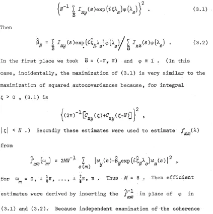
n

(Q, B) = iT1 I <KAsp{wy(s)-Bf(As; e)w.,(s)}

(1.12)

Here and elsewhere, ) is a sum over all €

B

and

8 S

18 ^ ^

The conditions we shall impose ensure that such values 0^, B^

(25)

l l ,

$(A ) = $ ( X )2$ ( X ) 2* i s a n . n . d . p ^ x p ^ H e r m i t i a n m a t r i x w i t h

$ ( - A ) = $ ( A ) ' , t h a t i s c o n t i n u o u s i n X o v e r B . F o r c o n v e n i e n c e i n o u r a s s u m p t i o n s o f § 2 . 2 we s h a l l a lw a y s t a k e y ( n ) a n d Z(tt) t o b e m e a n - c o r r e c t e d . I n p r a c t i c e t h i s may be a c c o m p l i s h e d by o m i t t i n g

fro m ( 1 . 1 2 ) t h e com p o n en t f o r s = 0 , w h ic h i n v o l v e s t h e d e v i a t i o n

~ I

W ( 0 ) - BT( 0 ;

6)w

( 0 ) = (/1//2tt) 2 { y -B f ( 0 ;

0)z}

.

y L S \

Q x M ß^ccr-e

Now b e c a u s e o f t h e sym m etry o f o , — i s - r e a l . Our p r o b le m h a s b e e n r e d u c e d t o one o f n o n - l i n e a r r e g r e s s i o n . W h ile c o n s i d e r a b l e p r a c t i c a l d i f f i c u l t i e s may b e a s s o c i a t e d w i t h t h e o p t i m i z a t i o n o f Qpj , t h e r e v o l u t i o n a r y d e v e lo p m e n t o f h i g h - s p e e d c o m p u t in g f a c i l i t i e s and t h e e x i s t e n c e o f s o p h i s t i c a t e d i t e r a t i v e p r o c e d u r e s make many s u c h t a s k s t e c h n i c a l l y f e a s i b l e .

The e x p r e s s i o n ( 1 . 1 2 ) i s a H e r m i t i a n fo rm i n W ( s ) w i t h m a t r i x

X

c o n s i s t i n g o f d i a g o n a l b l o c k s $ ( k ) . I t i s m o t i v a t e d i n t h e f o l l o w -s

i n g way. We s e l e c t some X € B an d some i n t e g e r m « N and c o n s t r u c t t h e f r e q u e n c i e s X. = 2ttJ /N , s = 1 , . . . 9 m , t h e

J s

i n t e g e r s J b e i n g c h o s e n s o t h a t t h e X . a r e c l u s t e r e d a r o u n d X .

s ° s

Then Hannan ( 1 9 7 0 ) h a s shown t h a t , u n d e r t h e a s s u m p t i o n s we s h a l l make f o r X(n) , t h e W ( j ) , s = 1 , . . . , m , c o n v e r g e t o i . i . d .

X s

c o m ple x v e c t o r s , (X)

m a t r i x o f x ( n ) , d e f i n e d a s i n ( 1 . 3 . 4 ) .

b e i n g t h e s p e c t r a l d e n s i t y

20

Thus a l t h o u g h t h e p a r e n t

19 I t i s i m p l i e d t h a t when t h e f u l l b a n d ( - T T , tt] i s u n d e r

c o n s i d e r a t i o n and N i s e v e n t h e com ponen t o f f r e q u e n c y Xg = tt i s e x c l u d e d , l e a v i n g o n l y N - 1 summands. T h i s i s n e c e s s a r y b e c a u s e i n g e n e r a l , an d i n t h e c a s e s i n w h ic h we a r e m o st i n t e r e s t e d ,

I m { f ( T T ;

**0)} * 0 .**

(26)

X(n) may be a u t o c o r r e l a t e d , f o r l a r g e N t h e summands i n ( 1 . 1 2 ) a r e r o u g h l y i n d e p e n d e n t a n d t h e p r o b l e m o f s e r i a l c o r r e l a t i o n may b e

C t — 1

e l i m i n a t e d . I f $ i s r e p l a c e d by f , when i t e x i s t s , i s a m o n o to n i c f u n c t i o n o f t h e l i k e l i h o o d b a s e d on i . i . d . n o r m a l W ( s ) ; h e u r i s t i c a l l y an o p t i m a l c h o i c e o f $ i s t h u s s u g g e s t e d . B e c a u s e

i s g e n e r a l l y unknown we a r e l e d t o d i s c u s s i t s e s t i m a t i o n i n

XX

§2.5.

Our f i r s t t a s k , h o w e v e r , i s t o i n t r o d u c e c o n d i t i o n s t h a t w i l l

/N / \ •

b e s u f f i c i e n t t o g i v e 0^ and c e r t a i n d e s i r a b l e p r o p e r t i e s , a s

w i l l b e shown i n

§§2.3, 2.4.

I n d i s c u s s i n g s p e c i a l c a s e s o f ( 1 . 1 ) i n s u b s e q u e n t c h a p t e r s we s h a l l t h e n b e a b l e t o a s s e r t s u c h p r o p e r t i e s w i t h l i t t l e o r no p r o o f and c o n c e n t r a t e on o t h e r a s p e c t s .

2.2 Some assumptions

I t i s w e l l known t h a t a s y m p t o t i c t h e o r y f o r n o n - l i n e a r r e g r e s s i o n s g e n e r a l l y r e q u i r e s r e s t r i c t i o n s on t h e p a r a m e t e r s . We c o n f i n e t h e a d m i s s i b l e 0 t o a s e t 0 d e f i n e d a s f o l l o w s . 21

k ( i ) Q i s the compact c l o s u r e o f a ( q - r ) - d i m e n s i o n a l C

mani f ol d. ,22 q > r >. 0 , k > 2 .

R e q u i r e m e n t s o f c o m p a c t n e s s o r b o u n d e d n e s s h a v e b e e n u s e d i n s i m i l a r c i r c u m s t a n c e s by J e n n r i c h ( 1 9 6 9 ) , M a lin v a u d (1 9 7 0 a , b ) , 21 T h r o u g h o u t , we i n d e x and r e f e r t o o u r a s s u m p t i o n s b y l o w e r - c a s e Roman n u m e r a l s ( i ) , ( i i ) e t c .

22 T h i s may b e d e f i n e d a s f o l l o w s . A u map, k > 0 , i s a

f u n c t i o n f m ap p in g an o pen s e t A oz r i n t o a f i n i t e - d i m e n s i o n a l v e c t o r s p a c e i f / p o s s e s s e s c o n t i n u o u s p a r t i a l d e r i v a t i v e s on A o f a l l o r d e r s 5 k . Then t h e open s e t V i s a ( q - r) - d i m e n s i o n a l

m a n i f o l d i f t h e r e e x i s t a f a m i l y o f p a i r s [ f. , V .) ( w h e re j

J J

i s an o pen s e t i n V and f . maps V . i n t o an

C J

) s u c h t h a t Ulf . = V an d f o r a l l n o n - d i s j o i n t ' :

f f vj n v k) - f k ( Vo n v k>

i s a ^

i s an i n d e x , V

.

J

o pen s e t i n

S

n

,

i

(27)

Hannan ( 1 9 7 1 a ) an d Dhrymes ( 1 9 7 1 a , b ) . The m o d i f i c a t i o n h e r e and i n R o b in s o n ( 1 9 7 2 ) i s t o a l l o w f o r t h e p r e s e n c e o f a n um ber o f g i v e n l i n e a r o r n o n - l i n e a r e q u a t i o n s i n 0 , w h ic h r e d u c e t h e d i m e n s i o n a l i t y o f t h e m a n i f o l d by t h e num ber o f i n d e p e n d e n t c o n s t r a i n t s . ( I f t h e s e e q u a t i o n s do n o t t h e m s e l v e s e s t a b l i s h c o m p a c t n e s s t h e l a t t e r r e s t r i c t i o n i s s u p e r i m p o s e d . ) We h a v e i n m ind c i r c u m s t a n c e s i n w h i c h , f o r e x a m p l e , 0 i s c o n f i n e d f o r t h e p u r p o s e o f n o r m a l i s a t i o n t o t h e s u r f a c e o f a

00

h y p e r s p h e r e o r e l l i p s o i d ( b o t h o f w h ic h a r e c om pact C m a n i f o l d s ) oJT 0 c o n s i s t s o f a n u m b er o f m u t u a l l y o r t h o g o n a l v e c t o r s . The n e e d t o a l l o w f o r s u c h c o n s t r a i n t s i s c r u c i a l i n §3, and f o r one r e a s o n o r a n o t h e r t h e y may a r i s e i n c o n n e c t i o n w i t h t h e o t h e r m o d e ls we

c o n s i d e r . We n o t e t h a t c o m p a c t n e s s , o r a t l e a s t b o u n d e d n e s s , may e n t e r i n a f a i r l y n a t u r a l way i n t o o u r c o n s i d e r a t i o n s : f i r s t , t o p r o d u c e i d e n t i f i c a t i o n i t may be n e c e s s a r y t o "b o u n d " 0 s i n c e B i s n o t c o n s t r a i n e d i n t h i s w ay; s e c o n d t o e n s u r e t h e s t a b i l i t y o f c e r t a i n f u n c t i o n a l e q u a t i o n s y s t e m s ( s e e §5). In any c a s e when t h e c h o i c e o f 0 i s n o t d e t e r m i n e d on p r i o r g r o u n d s i t may b e t a k e n a r b i t r a r i l y " l a r g e " , s u b j e c t t o o t h e r r e s t r i c t i o n s , i n w h ic h c a s e no p r a c t i c a l l i m i t a t i o n i s i n v o l v e d .

To a l l o w f o r t h e i n c o r p o r a t i o n o f a p r i o r i i n f o r m a t i o n , t o a s s i s t i d e n t i f i c a t i o n and a l s o t o f a c i l i t a t e t h e t a s k o f e x p r e s s i n g a num ber o f i n t e r e s t i n g m o d e ls i n t h e form ( 1 . 1 ) we a l l o w B t o s a t i s f y t h e hom ogeneous l i n e a r r e s t r i c t i o n s

3C = 0 , ( 2 . 1 )

w h e re C i s a m a t r i x o f g i v e n c o n s t a n t s , h a v i n g PjP^, row s an<^ l e s s t h a n p p ( p o s s i b l y z e r o ) l i n e a r l y i n d e p e n d e n t c o l u m n s , and

_L O

3 = v e c ' { B } . 23 The m a t r i x

2 3

(28)

L = I

PlP 3

C(C'C)

1 c l

projects onto the orthogonal complement of p^p^-dimensional vector

space spanned by the rows of C and (2.1) is implied by the relations 3 = 3L . (See Hannan, 1970, p. 416).

(ii) The processes x(£), z(£) have null mean vectors3 are mutually incoherent3 are stationary and ergodic and have absolutely continuous spectra and continuous spectral

density matrices. The sequences x(n), z(n) have

continuous spectral density matrices f^CA)., (A)

respectively 3 |A| 5 u , defined as in (1.3.4).

We have already explained the meaning of such conditions in §1.3.24

(iii) Uniformly in A € R 3 0 € 0 , f(A; 0) exists and is

given by (1.9). Uniformly in 0 6 0., f(A; 0) is

continuous in X 3 satisfying a Lipschitz condition of

order greater than one half. Uniformly in X € B

r(A; 0) is continuous in 0 .

The Lipschitz condition (see Zygmund, 1959, p. 43), needed for Theorem 2.B, is an unimportant restriction, every specific case of Y

we consider being differentiable in A and thus having modulus of continuity unity.

From (ii) and (iii) the relation

fy y W = e0)fzz(A)^ A > 6o)*Bi + fXX(A)

is integrable and thus (1.1) is well-defined in the m.s. sense. Hannan, 1970, p. 8.)

(2.2)

(C f .

(29)

Whereas (ii) is fundamental to our work stronger conditions on

z(t) will usually be needed because the attempt to estimate a continuous model from discrete data gives rise to an identification problem. Our estimation procedures are based on second-order

functions of the data and we ignore any information provided by

higher moments. Thus all we can attempt to estimate are the integer-lagged autocovariances between the elements of

[y(t

)1

* Z(t)'] , or equivalently the spectral density matrices

fi (A) ’

fJz(A) >

fzz(A) •

N S 1

7

•

Now from (2.2) we have, for X € B ,

(X)

=

I

B

f(X+2TTl;

0 )f£ Ut2irJ)f(X+2irZ; 0

)

*B’

+

f“x(X)

. (2.3) — 0 0

Also we have

r (X) =

b q

l r{\+

2

n-,

6

0) h z(x+

2

irn ,

(

2

.

4

)

J — 00

00

f2Z(X) = 1

lfzU+2lrt) ,

— 00

X C

B .

Now while we have information on f,,(X)

of isolating individual components

f

(X+2ttZ) .

we have no means

Thus there would

no hope of identifying 0 Q and from (2.3) and (2.4) without the

imposition of a further condition unless V is periodic of period 2tr ; T has the latter form for the unlagged regression (1.4)

(f(X; 0) E f(0)) and for the distributed lag system (1.8)

(30)

f 00 N

Bf(X; 0) = £ B(j )exp(£jA)

V _oo

Such models have formed the basis for

most regression analyses of time series, but they will not be of concern to us. When T is not periodic we need some way of choosing one out of the infinitely many Z(t) which generate the sequence Z

(n)

.

(iv) For A = ]i + 2t\l iJ ( ß j l = ±1, ±2, ... and for

I

X

I >

K

j

some K <

00 ^

q z u ) = o .

2 6 •

Under this condition there is no aliasing of the frequencies

6 , since (A) = f^z(A) » A € B ; any aliasing of

_ d

B n (-TT, 7T) is of no concern. (The extra requirement that be null everywhere outside an arbitrary finite interval is not practically restrictive but is needed in Theorems 2.5, 2.6.) When B = (—7T, TT) we thus require (A) = 0 , | A | > 7T , an assumption which is valid only if the sampling interval is sufficiently small to enable the detection of all frequency components of the continuous process. This "smoothness" assumption is strong, and one cannot adequately assess its validity without access also to data that are sampled at shorter intervals. Nevertheless in studying a continuous process it seems likely that one would sample with the intention of leaving a negligible spectral mass beyond the Nyquist frequency. For slow-moving economic series, for example, it may indeed be substantially concentrated in a much smaller band centred at the origin.

Henceforth^ when no confusion is possible3 we shall omit the superscript

26 A slightly stronger condition, used by Hannan and Robinson (1973), would require the spectral mass to be null for

(31)

d from th e s p e c tr a l d e n s i t i e s o f d i s c r e t e p r o c e s s e s . Then u n d e r ( i v ) , f o r X £ B

t , „ a > = Bnf 4 ; e0) f zz(A)f(A; eJ*B- + f vv(X) ,

(

2

.

5

)

yy

V

X) =

B

of 4; e0)fz2(X) .

0 ' 0 XX

(2.6)

M o r e o v e r , e v e n i f t h e s e r e l a t i o n s do n o t s e r v e t o i d e n t i f y 0^ and B , f (X) i s i d e n t i f i e d a s

U Ä Ä

f „(X) = f (X) - f (X)f (X)+f (X) ,

xx

yy

yz

zz

zy

5

b e c a u s e fro m ( 1 . 2 . 6 ) we may r e p l a c e f i n ( 2 . 5 ) by

f Z Z f+Z Z f Z Z f Z Z f Z Z and t h e n , fro m ( 2 . 6 ) , BQf ( X ; 0 Q) f z z f z z by f y z f z z

I n s o f a r a s t h e i d e n t i f i c a t i o n p r o b le m s te m s fro m a l i a s i n g i t i s r e s o l v e d by ( i v ) , b u t t h i s c o n d i t i o n i s b y no means s u f f i c i e n t t o e n s u r e t h e i d e n t i f i c a t i o n o f 0Q and BQ . T y p i c a l l y i n s y s t e m s whose r e d u c e d fo rm i s n o n - l i n e a r a num ber o f somewhat a r b i t r a r y

i d e n t i f i c a t i o n c o n d i t i o n s a r e r e q u i r e d , a n d t h e s e w i l l b e i m p l i e d by t h e f o l l o w i n g s t a t e m e n t .

( v ) U niform ly in a d m is s ib le (0 • 3) t (0n • $n )

t r{ ( 2 T T ) - 1 f [B0f(Xj 60) - Bf ( X; 0 ) ] f z z (X)[Bof(X; 60)

-Bf(X;

6)3**(X)dx\ >

0

.

(2.7)

(32)

a d m i s s i b l e (0 • ß) ^ (0 Q • 3 Q) a l m o s t e v e r y w h e r e i n a n o n - d e g e n e r a t e s u b s e t o f B ; s i n c e $ > 0 and > 0 u n i f o r m l y , t h e l e f t s i d e o f ( 2 . 7 ) i s n o n - n e g a t i v e a n d w i l l b e p o s i t i v e i f t h e m a t r i x i n t e g r a l h a s a n o n - z e r o e i g e n v a l u e , u n i f o r m l y i n a d m i s s i b l e

( 0 * 3 ) ^ (0q • ß ) . When we come t o c o n s i d e r s p e c i a l c a s e s o f ( 1 . 1 ) we s h a l l d i s c u s s t h e p a r t i c u l a r c o n d i t i o n s w h ic h w i l l p r o d u c e i d e n t i f i c a t i o n . However i t i s c o n v e n i e n t a t t h i s s t a g e t o comment g e n e r a l l y on t h e e f f e c t on t h e p o s s i b i l i t y o f i d e n t i f i c a t i o n o f t h e p r e s e n c e o f n o n - l i n e a r c o n s t r a i n t s , f o r w h i c h , a s a l r e a d y i n d i c a t e d , we s h a l l a l l o w . L o o s e l y s p e a k i n g , when a l l c o n s t r a i n t s a r e l i n e a r

t h e m o del i s e i t h e r ( g l o b a l l y ) i d e n t i f i e d o r t h e r e e x i s t s a n o n - d e n u m e r a b l e s e t o f a l t e r n a t i v e (0 • 3 ) a d m i s s i b l e i n t h e s e n s e

( d i f f e r e n t fro m t h a t a b o v e ) t h a t ( 2 . 7 ) i s u n t r u e . When 0 s a t i s f i e s a num ber o f n o n - l i n e a r e q u a t i o n s t h e n a l t h o u g h t h e m odel may n o t be

g l o b a l l y i d e n t i f i e d i t i s p o s s i b l e t h a t t h e r e e x i s t o n l y a f i n i t e o r d e n u m e r a b l e num ber o f a l t e r n a t i v e a d m i s s i b l e s t r u c t u r e s . In t h i s c a s e , when t h e r e e x i s t s a n e i g h b o u r h o o d o f t h e t r u e p a r a m e t e r v e c t o r c o n t a i n i n g no o t h e r a d m i s s i b l e v e c t o r , t h e m odel i s s a i d t o be

l o c a l l y i d e n t i f i e d . ( S e e f o r e x a m p le W ald, 1 9 5 0 , F i s h e r , 1 9 6 6 , C h a p t e r 5 . ) T h e n , a t l e a s t i n p r i n c i p l e , 0 may b e c h o s e n t o i n c l u d e one an d o n l y one o f t h e a d m i s s i b l e v e c t o r s a n d g l o b a l i d e n t i f i c a t i o n i s a c c o m p l i s h e d .

2 . 3 The s t r o n g law o f l a r g e numbers

We p r o v e f i r s t a t h e o r e m o f f u n d a m e n t a l i m p o r t a n c e t o much o f w h a t f o l l o w s .

THEOREM 2 . 1 . For k , l = 1, 2 d e f i n e

=

^ _1

I

^ ( w) ^( w+ j ) *

Y ^ ( j ) = (

ei'

i

'

kfkl(\)d\

3

(33)

I V1

(s) =

( 2ttN) 1

I I

L( m) ^^( n) e xp{ i ( m- n) X } ,

' kt

_m,m

₌₁

0„(Bi

<p) =

N'*

1 I

I . , ( s ) ( p U ; 0) , ff( 6 ; <p) = (2Tt)- 1 7c Z

- \

n

< s

< [ f t f ] ,

/ ^^( X) c p( X; 0)dX ,

B

where

(p( X ; 0) i s a

complex-valued funotion th a t is continuous in

X j

uniformly in

0 €

0

j

and

continuous in

0

uniformly in

X £

B .

Let

l i m a

ft-** k l U ) = YfeZ( j ' ) a . s . ,

( 3 . 1 )

k , l = 1 , 2 j uniform ly in f i x e d i n t e g r a l j 3 0 < \ j \ < N 3 and l e t

f ‘k i (X) be continuous in X . Then £/* c o n d itio n ( i ) h o ld s 3 27

l i m ^ „ ( 0 ; cp) = # ( 0 ; cp) , a . s . , /I/-*»

uniform ly in 0 £ 0 .

Proof.

I t i s c o n v e n i e n t t o f i r s t p r o v e p o i n t w i s e c o n v e r g e n c e w i t h B r e p l a c e d by (-7T, T T ] an d cp( X; 0 ) t a k e n t o b e c o n t i n u o u s a n d p e r i o d i c o f p e r i o d 2tt . Then a l t h o u g h t h e F o u r i e r s e r i e s o f (p may n o t be

a b s o l u t e l y c o n v e r g e n t , s i n c e (p i s c o n t i n u o u s i t s «7th f i r s t - o r d e r C e s a r o m e an ,

cPj-(X; 0) = ( 2tt)

c o n v e r g e s u n i f o r m l y i n X t o cp , w h e r e by F T(X) we s h a l l a l w a y s tl

<p(y; 0 ) ^ j - ( X - y ) d y , ( 3 . 2 )

mean F e j e r ’ s k e r n e l

FjiX) = «7

( S e e Zygmund, 1 9 5 9 ,

i i d - 1 . 2

l e ^ X

=

y

J = 0 \ j \ < J p . 8 9 . ) Then f o r g i v e n

s u p I<p( X; 0 ) -cPcj ( X ; 0) I

( i .

e > 0

< e

( 3 . 3 )

f o r «7 s u f f i c i e n t l y l a r g e . Thus

27 '