Cone-based joint sparse modelling for hyperspectral image classification

City, University of London Institutional Repository

Citation

:

This is the accepted version of the paper.

This version of the publication may differ from the final published

version.

Permanent repository link: http://openaccess.city.ac.uk/21062/

Link to published version

:

Copyright and reuse:

City Research Online aims to make research

outputs of City, University of London available to a wider audience.

Copyright and Moral Rights remain with the author(s) and/or copyright

holders. URLs from City Research Online may be freely distributed and

linked to.

City Research Online: http://openaccess.city.ac.uk/ [email protected]

Cone-based Joint Sparse Modelling for Hyperspectral

Image Classification

Ziyu Wanga,b, Rui Zhuc, Kazuhiro Fukuid, Jing-Hao Xueb,∗

a_{Department of Security and Crime Science, University College London, UK} b

Department of Statistical Science, University College London, UK

c_{School of Mathematics, Statistics and Actuarial Science, University of Kent, UK} d

Department of Computer Science, University of Tsukuba, Japan

Abstract

Joint sparse model (JSM) is being extensively investigated on hyperspectral

images (HSIs) and has achieved promising performance for classification. In

JSM, it is assumed that neighbouring hyperspectral pixels can share sparse

representations. However, the coefficients of the endmembers used to

recon-struct a test HSI pixel is desirable to be non-negative for the sake of physical

interpretation. Hence in this paper, we introduce the non-negativity

con-straint into JSM. The non-negativity concon-straint implies a cone-shaped space

instead of the infinite sample space for pixel representation. This leads us to

propose a new model called cone-based joint sparse model (C-JSM), to

in-stall the non-negativity on top of the sparse and joint modelling. To solve the

C-JSM problem, we also propose a new algorithm through introducing the

non-negativity constraint into the simultaneous orthogonal matching pursuit

(SOMP) algorithm. The new algorithm is called non-negative simultaneous

orthogonal matching pursuit (NN-SOMP). Experiments and investigations

∗

Corresponding author.

Email addresses: [email protected](Ziyu Wang),[email protected](Rui

Zhu),[email protected](Kazuhiro Fukui),[email protected](Jing-Hao

show that the proposed C-JSM can produce a more stable, sparse

represen-tation and a superior classification than other methods which only ensure

the sparsity, non-negativity or spatial coherence.

Keywords: Hyperspectral image classification, joint sparse model,

simultaneous orthogonal matching pursuit, cone, non-negativity.

1. Introduction

Sparse representation has been proven to be superiorly effective for a

wide range of applications in computer vision, pattern recognition and signal

processing [1, 2]. It is based on the assumption that most natural signals

can be compactly represented by a linear combination of only a few basis

vectors (aka atoms) from an over-complete dictionary.

Recently, sparse representation has been extensively investigated in

hy-perspectral imaging [3–14]. A hyhy-perspectral image (HSI) is a 3-dimensional

data cube with two spatial dimensions and one spectral dimension. From the

view of the spectral dimension, each HSI pixel is a vector, namely spectral

signature whose elements correspond to reflectances at different wavelengths

(spectral bands). Different classes of spectral signatures can have distinct

reflectances at specific wavelengths and, as a result, the spectral signatures

can provide discriminative information for classification. The sparse

repre-sentation of an HSI pixel is accomplished by a linear combination of atoms

in a spectral dictionary. The sparse model can be approximately solved

by greedy algorithms such as orthogonal matching pursuit (OMP) [15] (l0

-norm based methods) or by convex optimisation problems such as the Lasso

(l1-norm based methods). In such sparse representation, the dictionary is

usually constructed by the training spectral signatures directly from HSIs

dictionary learning has been also investigated for HSI analysis. Details of

how to design and learn quality dictionaries for HSI classification can be

found in [16–20], for example.

One step further, by virtue of the signal coherence in HSIs, a joint sparse

model (JSM) has been successfully developed for HSI classification and has

achieved promising performance [3]. The underlying assumption of JSM is

that all HSI pixels in a small spatial neighbourhood can be jointly

approx-imated by sparse linear combinations of a few common training samples,

i.e. the neighbourhood shares a common sparse model. The original JSM

proposed by [3] adopts a square window centred on a test pixel for joint

modelling; a greedy algorithm, namely simultaneous orthogonal matching

pursuit (SOMP) [21], is used to solve JSM. On top of this JSM, some

ex-tensions have been proposed to overcome the limitations of JSM [4–9]. To

extend JSM for linearly non-separable class samples, the kernel versions of

SOMP have been studied in [4, 5]. To enhance JSM with a more effective

neighbourhood, the adaptive versions of JSM have been proposed in [6–9],

which aim to produce shape/size adaptive local windows for JSM.

An important property of hyperspectral signals is the non-negativity,

for both the signal itself and the abundance coefficients. It has been

inten-sively considered for problems of HSI unmixing [22–36]. A large number

of these reports have been focused on the non-negative matrix factorisation

(NMF), a typical decomposition method for the HSI unmixing problems.

NMF decomposes the sample data matrix into two low-dimensional

matri-ces serving as endmembers and coefficients, both of which are enforced to

be non-negative. The underlying assumption of the NMF-based unmixing

is that mixed HSI pixels can be decomposed into a collection of

the endmembers, which characterise the reflected electromagnetic energy of

specific materials, should be non-negative. In addition, the proportions of

the underlying physical materials (endmembers) should be non-negative for

physical interpretations.

From the representation point of view, a reconstructed HSI pixel by the

sparse representation should be as similar as possible to the original signal,

therefore is desirable to be non-negative with respect to physical

interpreta-tions. To this end, the sparse coefficients should be non-negative so long as

the atoms of dictionary are non-negative. In most settings of sparse

repre-sentation, the dictionary atoms are either constructed directly by the pixels

in an HSI, or from a well-defined library, i.e. endmembers. Work in [37]

also focuses on learning non-negative dictionaries for better representative

power. This means the dictionary atoms are non-negative and hence it is

reasonable to impose the non-negativity constraint on the coefficients. It

is known that the non-negative coefficients estimation induces a cone-shape

representation. In line with this, our recent work [38, 39] demonstrates the

reasoning and appropriateness of the non-negative constraint on the

coef-ficients, as well as the Bayesian derivations of cone-representation for HSI

target detection.

However, research of sparse representation for HSI classification,

partic-ularly the JSM-based methods in [3, 6–9], have not incorporated the

non-negativity properties of HSI. To fill in this gap, through replacing the signal

representation of JSM by cone representation, in this paper we incorporate

non-negativity into HSI classification and propose a new HSI classification

model called cone-based joint sparse model (C-JSM).

Methodologically, inspired by the NMF for HSI unmixing, we devise the

classifi-cation. Since the given atoms of a dictionary are constructed directly by

the HSIs or from spectral libraries, it implies that the dictionary atoms

are non-negative. In this fashion, both endmembers and coefficients are

non-negative, and thus the proposed C-JSM considers both sparsity and

non-negativity, making the joint sparsity recovery problem more realistic in

terms of interpretation. It will be illustrated to have a more sparse and

stable representation than the conventional JSM.

Computationally, we propose a new algorithm called non-negative

si-multaneous orthogonal matching pursuit (NN-SOMP) to solve the C-JSM

problem. The proposed NN-SOMP algorithm is developed on the basis of

the SOMP algorithm with an additional non-negative constraint on the

co-efficients, which will be illustrated easy to implement in this paper.

In short, the main contribution of this paper can be summarised as

fol-lows: 1) we incorporate the non-negativity constraints into JSM to consider

more realistic physical characteristics of the spectral signals and propose a

new HSI classification model called C-JSM; 2) we also propose a new

NN-SOMP algorithm to solve the optimisation problem of C-JSM; and 3) C-JSM

produces a stable sparse representation as well as a superior classification

performance.

The rest of the paper is organised as follows. Section 2 reviews the sparse

model (SM) and the joint sparse model (JSM) for the HSI classification.

Section 3 introduces the cone-based model and the cone-based sparse model.

In section 4, the proposed C-JSM, as well as the proposed algorithm

NN-SOMP to solve the C-JSM problem, are detailed. Experimental studies

in section 6 demonstrates the superior classification performance of C-JSM

over the compared methods on two real hyperspectral datasets. Finally this

2. Joint sparse models for HSI classification

2.1. Sparse model

Given an unknown B-dimensional signal x∈_RB _{and a dictionary}

con-structed by N training samples (also termed atoms) D = [d1, . . . ,dN] ∈

RB×N with B < N, the sparse model is formulated as finding a sparse

coefficient vectorα∈RN that

x≈Dα. (1)

The sparse coefficient vector α implies that the signal is approximated

by the linear combination of only a small number of (e.g. at mostL) atoms

inD. It can be estimated by solving the following optimisation problem:

ˆ

α= argmin

α

kx−Dαk₂, s.t. kαk₀ ≤L. (2)

In (2),kαk₀ denotes al0-pseudo-norm ofα, which indicates the number

of non-zero elements in α; and L(LN) denotes the sparsity level of the

model. The problem in (2) is NP-hard, but it can be approximately solved

by greedy algorithms such as orthogonal matching pursuit (OMP) [15], or

be relaxed by replacing the l0-pseudo-norm with the l1-norm such as the

Lasso. It is worth noting that the dictionaryD have unitl2-norm columns.

2.2. Joint Sparse model (JSM)

In HSIs, local smoothness and sparsity are often assumed, because

neigh-bouring pixels in a small area often consist of similar materials and the

classes of these materials are few. The joint sparse model (JSM) is proposed

under these assumptions, with all neighbouring pixels around a central pixel

Instead of sparsely representing a single signal vectorx∈_RB_{, the JSM is}

designed to model for a matrixX∈_RB×T _{of T signals simultaneously, and}

assumes that the signals share a common sparse pattern. In the classification

of HSI, the matrixXdenotes a small window centring on a test pixelxcand

consisting ofT HSI pixels, with each pixelxtfort= 1, . . . , T represented by

aB-dimensional vector forB spectral bands. TheT pixels in the window are

jointly approximated by sparse linear combinations of atoms from a given

over-complete dictionary D:

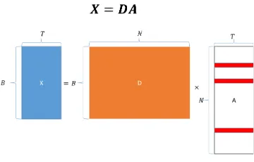
X= [x1, . . . ,xT]≈D[α1, . . . ,αT] =DA, (3)

where A ∈RN×T is the matrix of unknown coefficients [α1, . . . ,αT]. It is

assumed that the coefficient vectors share the same sparsity pattern, i.e.A

only containsL(LN) non-zero rows.

The estimation of A can be achieved by solving a joint sparse recovery

problem:

ˆ

A= argmin

A

kX−DAk2_F , s.t. kAk_row,0 ≤L, (4)

wherek·k_F denotes the Frobenius norm; andkAk_row,0 denotes the row-wise

l0-pseudo-norm, which is the number of non-zero rows ofA. An illustration

of the JSM equation is shown in Figure. 1. As with (2), problem (4) is

NP-hard and it can be approximately solved by greedy algorithms such

as simultaneous orthogonal matching pursuit (SOMP) algorithm [21]. The

Figure 1: An illustration of JSM, whereXis aB×T matrix denoting a small window

consisting ofT HSI pixels,Dis aB×N matrix representing an over-complete dictionary

withN atoms; andAis anN×T coefficient matrix with onlyLnon-zero rows. The red

lines inAindicate the non-zero rows and the blank areas indicate zero rows ofA.

2.3. Classification rules of SM and JSM

For the SM, the class ofxis determined by applying the obtained sparse

coefficient vector ˆα from (2). We define the class-wise residuals as

rm(x) =kx−Dmαˆmk2₂, m= 1, . . . , M, (5)

where M is the total number of classes, ˆαm contains the Nm elements in

ˆ

α that are associated with sub-dictionary Dm of the mth class, with N =

PM

m=1Nm. The label of the test pixelxis determined by its minimal residual

over allM classes:

Class(x) = argmin

m=1,...,M

rm(x). (6)

For the JSM, once the sparse coefficient matrix ˆA is obtained from (4),

we calculate the class-wise residual of the matrixX from its class-wise

ap-proximation similar to (5):

rm(X) =

X−D

m_Aˆm

2

In (7), there are Nm rows in ˆA corresponding to a sub-dictionary Dm and

N = PM

m=1Nm. Different from the SM, the label of the central test pixel

xcin window Xis jointly determined by the minimal residual of Xover all

M classes, i.e.

Class(xc) = argmin

m=1,...,M

rm(X). (8)

3. Cone-based sparse model

3.1. Cone-based model

A cone model (CM) to represent vectors xis defined as

C:

(

x|x=

N

X

i=1

αidi=Dα, αi ≥0

)

, (9)

whereαiis thenon-negativecoefficient of atomdi, andαis anN-dimensional

vector ofnon-negative coefficients.

The non-negative coefficient vector αis estimated by solving the

follow-ing optimisation problem:

ˆ

α= argmin

α

kx−Dαk2₂, s.t. α≥0, (10)

where α ≥ 0 denotes that every single element of the vector α should be

non-negative. Problem (10) can be solved by the active-set methods, such

as the typical non-negative least square method (NNLS) [40] (MATLAB

functionlsqnonneg) and its extension fast-NNLS (fnnls) [41]. In this paper, we use the CM (10) as a baseline method for HSI classification. Specifically,

(10) is used for the representation of a single test HSI pixel. The label of a

3.2. Cone-based sparse model

For the l0-pseudo-norm optimisation problem, the non-negative

orthog-onal matching pursuit (NN-OMP) algorithm has been investigated in [42],

which introduces the non-negativity constraint into the conventional OMP

algorithm. Technical details of the algorithm vary, depending on different

criteria such as fast implementation [43].

In [42, 43], a desired coefficient vector α is estimated by solving the

following optimisation problem:

ˆ

α= argmin

α

kx−Dαk2₂+kαk₀, s.t. α≥0, (11)

which is forced to be sparse and non-negative.

In this paper, we term model (11) the cone-based sparse model

(short-ened as CSM). To our knowledge, CSM is first introduced and studied in

this paper for HSI classification. To align with the rule of SM (2), the

classification of an HSI based on CSM (11) is also determined by (6).

4. Cone-based joint sparse model (C-JSM) for HSI classification

We notice that, on the one hand, SM (2), CM (10) and CSM (11) are

all constructed for a single test HSI pixel and do not take the spatial

co-herence [44] into consideration; while on the other hand, JSM accounts for

the neighbouring spatial information, but the coefficients estimated by JSM

are only assumed to be sparse, not necessarily non-negative. As with the

underlying assumptions made for HSI unmixing, an HSI pixel can be

de-composed into a collection of endmembers with non-negative proportions.

The endmembers are spectral signatures which characterise the reflect

the case of HSI classification, the dictionary atoms are usually constructed

directly from the HSI or from the spectral libraries, so the atoms can be

assumed acting as endmembers, which inspires us to devise a cone-based

representation for the joint models for a more realistic interpretation.

In the same notation as aforementioned, the cone-based representation

of a test windowX∈_RB×T _{can be formulated as follows:}

X≈DA, s.t. A≥0, (12)

whereA is anon-negative coefficient matrix andA≥0denotes that every

element ofA should be non-negative. To estimateA, problem (12) can be

reformulated as

ˆ

A= argmin

A

kX−DAk2_F, s.t. A≥0. (13)

In this paper, we term model (12) the joint cone model (shortened as JCM).

We also utilise it as a baseline method.

The optimisation problem (13) can be solved by two algorithms. Firstly,

the reconstruction of each column vector xt for t = 1, . . . , T can be solved

independently by the conventional NNLS [40] or fast-NNLS [41]. Secondly, it

can be solved by an algorithm called fast combination NNLS (FC-NNLS) [45],

which is proposed to solve the large-scaled non-negativity-constrained least

square problems. It solves a set of linear reconstruction for X in a parallel

fashion instead of solving a set of single x in a serial fashion. Specifically,

it rearranges the calculations in the standard active-set NNLS on the basis

of combinational reasoning and reduces the computation burden for NNLS

win-dow size T in our case. The estimated coefficient matrices ˆXs obtained by

these two methods are the same. So we can regard FC-NNLS as a fast

implementation of NNLS for solving the JCM problem (13).

Incorporating JCM (13) into the JSM for HSI classification (4), we

pro-pose a new method as

ˆ

A= argmin

A

kX−DAk2_F ,

s.t. kAk_row,0≤Land A≥0.

(14)

We call this new model (14) the cone-based joint sparse model (shortened

as C-JSM). In short, the proposed C-JSM incorporates the non-negative

constraints into the sparse representation of a test windowX by joint

mod-elling. The coefficient matrix A of the test window X is not only sparse,

but also forced to be non-negative. On top of these two desirable properties,

the spatial coherence of HSI is also reflected in that the coefficient vector

of the central test pixel xc is jointly determined by those HSI pixels in its

local neighbourhood with the same non-negative and sparse constraints. As

a result, HSI pixels in the local windowX share the same basis vectors of a

cone, and the sparsity of the coefficients are determined only in the region

of the cone.

Same as JSM, the two cone-based sparse models, JCM and C-JSM, are

also joint models, hence we adopt the classification rule (8) for them. To

solve the C-JSM problem (14), we propose a new algorithm and detail it in

5. Algorithm of NN-SOMP for solving C-JSM

We propose a new algorithm called non-negative simultaneous

orthogo-nal matching pursuit (NN-SOMP), to solve the C-JSM problem. It combines

the NNLS-based methods and the SOMP algorithm together to produce a

non-negative and sparse estimation of the coefficient matrix ˆAin (14).

Be-fore introducing the proposed NN-SOMP, we first present the non-negative

OMP to get an insight of the paradigm.

5.1. Algorithm of NN-OMP

The traditional SM in (2) with the l0-pseudo-norm constraint on the

coefficient vector is approximately solved by greedy algorithms, of which

one of the most popular algorithms is called orthogonal matching pursuit

(OMP) [15]. We assume that the columns (atoms) of the dictionary D are

normalised so that kdik2 = 1 for i = 1, . . . , N. At the beginning of the

algorithm, a residual vectorr0 is initialised to be the test HSI pixelx. The

OMP iteratively selects at each step the column ofD, i.e. the atomdi, which

has not been selected but is most correlated with the residualsrj−1, where

j is the current iteration number. The maximal correlation is calculated

asdT_i r_j−1

, which is the absolute value of the projection of residual vector

rj−1 onto the the atomdi. The selected atomdi is then added into the set

of selected atoms. The algorithm updates the residual vector by

project-ing the observed vector x onto the linear subspace spanned by the atoms

that have already been selected, and then iterates. The termination of the

OMP algorithm is either conducted by setting the iteration number, i.e. the

sparsity levelL, or by setting a thresholdτ of the residual.

Based on the OMP algorithm, the non-negative OMP (NN-OMP) is

into the iterations. The main difference between OMP and NN-OMP is

the updating criteria of residual vector rj. In OMP, the residual vector is

updated by rj =x−DΛjβˆj, where the coefficient vector βj is obtained by

least squares (LS) and has a closed-form solution. However in NN-OMP, to

guarantee non-negative coefficients, the coefficient vector β_j at iteration j

should be solved by NNLS-based methods instead of the LS method, which

is described in (16). Hence there is no closed-form solution for β_j. The

algorithm of NN-OMP used in this paper is summarised in Algorithm 1.

Other versions of NN-OMP can be found in [42, 43]. We note that there is

a slight difference between Algorithm 1 and the algorithms proposed in [42,

43]: we use the absolute value dT_ir_j−1

instead of the maximal positive

value max(dT_i rj−1) > 0 used in [42, 43]. Although these two approaches

may select different atoms from iteration 2 (for iteration 1,r0 and di both

are positive so the produced results are same), the size of residuals krjk₂

can be reduced iteratively by both, which reflects the core idea of matching

pursuit algorithms. It may not be easy to claim which approach is more

appropriate. To align with the original framework of OMP and for a clearer

comparison, we only change the updating of the coefficients by (16) and

adopt Algorithm 1 as a representative of NN-OMP algorithm in the following

discussion.

5.2. Algorithm of NN-SOMP

Following the derivation of NN-OMP from OMP, we propose a new

al-gorithm called NN-SOMP, which combines the SOMP alal-gorithm [21] and

the NNLS-based methods together to solve the problem of C-JSM (14).

The SOMP algorithm [21] is a generalised OMP algorithm. It aims

Algorithm 1 The NN-OMP algorithm to solve CSM (11).

Input: • Dictionary D = [d1, . . . ,dN]∈ RB×N with kdik2₂ = 1 for i=

1, . . . , N.

• A test pixelx∈_RB_.

• Sparsity levelL or thresholdτ.

Output: A non-negative and sparse coefficient vector ˆα.

Initialisation:

• The residual vector r0=x.

• Sparse index set Λ0 =∅.

• Iteration counter j= 1.

while j6L orkrj−1k2₂< τ do

(1) Find an index λj that solves the easy optimisation problem:

λj = argmax i=1,...,N

dT_i r_j−1

. (15)

(2) Update the index set Λj = Λj−1∪ {λj}.

(3) Determine non-negative coefficient vectorβ_j by the NNLS algorithm in the coneC whose basis vectors are the atoms ofDindexed in Λj:

ˆ

β_j = argmin

βj

x−D_Λjβ_j

2

2,s.t. βj ≥0, (16)

whereDΛj ∈R

B×j _{consists of thej atoms in D indexed in Λ} j.

(4) Determine the new residual:

rj =x−DΛjβˆj. (17)

(5) j←j+ 1.

end while

Compute the non-negative and sparse coefficient vector ˆαwhose non-zero elements are indexed by Λ and the corresponding L elements of vector

ˆ

columns of matrix X, by using different linear combinations of the same

atoms of the dictionary. The algorithm balances the error in approximation

against the total number of atoms that participate. Specifically, the atoms

supporting the sparse solution are sequentially selected from the dictionary.

At each iteration, the atom that simultaneously yields the best yet simple

approximation to all of the residual vectors is selected. Particularly, at the

jth iteration, we calculate an N ×T correlation matrix Corr = DTRj−1,

where Rj−1 is a residual matrix between the test window X ∈ RB×T and

its approximation from the last iteration. The (i, t)th entry in Corr is the

correlation between the ith dictionary atom di and the residual vector for

xt, where t = 1, . . . , T at the current iteration j. In the algorithm, the

lp-norm, where p ≥ 1, for each of the N rows of Corr is computed. The

row index corresponding to the largestlp-norm is then added into the sparse

index set of selected atoms. As mentioned in [3], different values ofp have

been adopted in literatures, such asp= 1 is in [21],p= 2 in [46] andp=∞

in [47]. In this paper we use p =∞ to align with [47]. Similarly to OMP,

the termination of the SOMP algorithm is either conducted by setting the

iteration number, i.e. the sparsity levelL, or by setting a threshold τ of the

size of the residual. Details of the SOMP algorithm can also be found in [3].

The proposed NN-SOMP algorithm is devised on the basis of the SOMP

algorithm; it incorporates non-negative constraints in the simultaneous

ap-proximation of a test window X and is summarised in Algorithm 2. We

replace the LS-based estimates of the coefficient matrix of SOMP by the

NNLS-based estimates (19). We can see that (19) in our proposed

algo-rithm is in fact a standard JCM problem as in (13).

As aforementioned, the optimisation problem (19) can be solved by two

implementa-tion, each column of X can be treated independently. Specifically,

prob-lem (19) in the Algorithm 2 is broken into T individual NNLS problems

formulated by (10). TheseT problems can be solved by conventional NNLS

algorithm [40] or fast-NNLS algorithm [41]. Then the coefficient matrix ˆPj

is obtained by concatenating the estimated coefficient vectors column by

col-umn. In this fashion, we need to use an inner FOR loop to compute step (3)

of the NN-SOMP algorithm (Algorithm 2). The optimisation problem (19)

can also be solved by the FC-NNLS algorithm [45], which is a generalised

NNLS algorithm. It aims to solve the non-negative least squares with

mul-tiple input vectors. FC-NNLS rearranges the selection of the support set,

and reduces substantially the computational burden required for the NNLS

problems which have large numbers of observation vectors.

The conventional NNLS algorithm utilises the active/passive set method

to solve an inequality-constrained least squares problem as a sequence of

equality-constrained problems, also termed “column-serial” [45]. FC-NNLS

is also based on this NNLS scheme. In general, the overall NNLS in the

FC-NNLS is responsible for defining the sequence, but sequentially

solv-ing the problem tends to be computationally inefficient as it can result in

redundant calculations. To this end, FC-NNLS solves the problem in a

“column-parallel” fashion. Specifically, the algorithm firstly groups

prob-lems that share a common passive set and solve them together, and then

recognises that the passive sets vary from iteration to iteration. Each NNLS

iteration for all columns are performed in parallel rather than performing all

iterations for each column in series. Note that columns will require different

numbers of iterations to achieve optimality. The conventional NNLS and the

FC-NNLS produce the same estimation results; for a faster computation, we

Algorithm 2 The NN-SOMP algorithm to solve C-JSM (14).

Input: • Dictionary D = [d1, . . . ,dN]∈ RB×N with kdik2₂ = 1 for i=

1, . . . , N.

• A test windowX= [x1, . . . ,xT]∈RB×T.

• Sparsity levelL.

Output: A non-negative and sparse coefficient matrix ˆA.

Initialisation:

• The residual matrix R0 =X.

• Sparse index set Λ0 =∅.

• Iteration counter j= 1.

while j6L orkRj−1k2_F < τ do

(1) Find an indexλj that solves the following easy optimisation problem:

λj = argmax i=1,...,N

RT_j−1d_i

p, p≥1. (18)

(2) Update the index set Λj = Λj−1∪ {λj}.

(3) Determine non-negative coefficient matrix Pj by the NNLS-based

algorithm in the cone C whose basis vectors are the atoms of D

indexed in Λj:

ˆ

Pj = argmin

Pj

X−D_ΛjP_j

2

F ,s.t. Pj ≥0, (19)

where DΛj ∈ R

B×j _{consists of number of j atoms in D indexed}

in Λj. Optimisation problem (19) can either determined in a serial

fashion that each column of X is treated independently and can be approximated by NNLS [40] or fast-NNLS [41]; or in a parallel fashion by FC-NNLS [45]. The two approaches produce the same result.

(4) Determine the new residual matrix:

Rj =X−DΛjPˆj. (20)

(5) j←j+ 1.

end while

6. Experiments

In this section, we investigate the performance of the proposed C-JSM

method on HSI classification. The experiments are carried out on two

well-known real HSI datasets: the AVIRIS Indian Pines dataset and the ROSIS

University of Pavia dataset, both of which can be downloaded from [48].

6.1. Methods compared

We evaluate the proposed C-JSM (14) and compare it with five

base-line methods: the sparse model (SM) (2), the joint sparse model (JSM) (4),

the cone model (CM) (10), the cone-based sparse model (CSM) (11) and

the joint cone model (JCM) (13). Corresponding algorithms used to learn

these models are listed in Table 1: the proposed NN-SOMP (Algorithm 2),

OMP [15], SOMP [21], NNLS [40], NN-OMP (Algorithm 1) and FC-NNLS [45],

respectively.

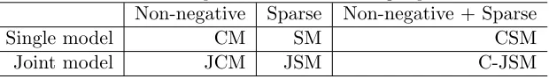
Table 1: Compared methods and their corresponding algorithms: CM – cone model; SM – sparse model; CSM – cone-based sparse model; JCM – joint cone model; JSM – joint sparse model; C-JSM – cone-based joint sparse model.

Meth. CM SM CSM JCM JSM C-JSM

Alg. NNLS OMP NN-OMP FC-NNLS SOMP NN-SOMP

From the point of view of models, these six methods can be grouped

into two types of models: single models (CM, SM, and CSM) and joint

models (JCM, JSM and C-JSM). The single models label a test HSI pixel

by considering only the test pixel, i.e. a vector x in (2), (10) and (11),

whereas the joint models label a central test HSI pixelxc by considering a

local window around it, i.e. a matrixX in (4), (13) and (14). The labelling

by the single models is determined by (6), whereas the labelling by the joint

according to their constraints on non-negativity and sparsity: CM and JCM

are only with the non-negativity constraint; SM and JSM are only with the

sparsity constraint; and CSM and C-JSM both consider the non-negativity

and sparsity simultaneously. Details of the relationships among the methods,

algorithms, models and constraints are presented in the confusion matrices

in Table 2 and Table 3.

Table 2: Compared methods and their groups.

Non-negative Sparse Non-negative + Sparse

Single model CM SM CSM

Joint model JCM JSM C-JSM

Table 3: Compared algorithms and their groups.

Non-negative Sparse Non-negative + Sparse

Single model NNLS OMP NN-OMP

Joint model FC-NNLS SOMP NN-SOMP

6.2. Performance measures

We evaluate the performances of the compared methods by using three

standard measures for HSI classification: the overall accuracy (OA), the

average accuracy (AA) and kappa coefficient κ [49], which are widely used

by the remote sensing community.

The OA,AAand κ are defined as follows:

OA= Ncorr

Ntest

, AA= 1

M

M

X

m=1

N_mcorr

Nclass m

and κ= OA−pe 1−pe

. (21)

In (21), the overall accuracy (OA) is defined as the ratio of the number of

the correctly-classified test pixelsNcorr over the total number of test pixels

accuracies of the M individual classes, where N_mclass is the total number of

test pixels of classm, andN_mcorr is the number of the correctly-classified test

pixels of class m. The κ coefficients measures the percentage of classified

test pixels corrected by the number of agreements that would be expected

purely by change [49]. In (21), we havepe=PM_m=1(Fm×Fmt), whereFm is

the ratio of data assigned to classm by the classifier andF_mt is the ratio of

data that belong to classm.

6.3. Parameter settings

Among the compared methods, in single models, only one unknown

pa-rameter needs to be determined, i.e. the sparsity level L; in joint models,

two unknown parameters are involved, the sparsity levelL and the window

size T, except for FC-NNLS in which only the window size T is involved.

The values of the parameters for all methods are determined via the

leave-one-out cross validation (LOOCV) in the training phase.

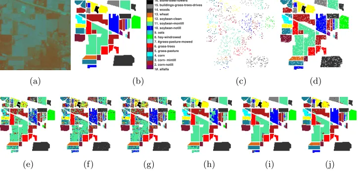
6.4. Real dataset: Indian Pines

The AVIRIS Indian Pines dataset consists of 145×145 pixels from 200

spectral bands after removing the water absorption bands. There are sixteen

classes of materials in the scene. For each of the 16 ground-truth classes,

we randomly choose about 9% of labelled pixels as the dictionary, i.e.D ∈

R200×957. The rest pixels are used for testing, i.e.Xtest∈R200×9409. Similar

experiment settings can also be found in [3–9, 16–18, 20] with different

training/test samples and accordingly non-identical performance.

A summary of the numbers of training and test pixels for individual

classes is given in Table 4. The false colour of the image averaging through

all the bands, the 16 ground-truth classes, the training set and the test set

Table 4: The Indian Pines dataset: Ground-truth label, class material, training set and test set. We use around (9% of all pixels) for training and the rest for testing.

Class Material Training Test

1 Alfalfa 5 49

2 Corn-notill 132 1302

3 Corn-mintill 77 757

4 Corn 22 212

5 Grass-pasture 46 451

6 Grass-trees 69 678

7 Grass-pasture-mowed 3 23

8 Hay-windrowed 45 444

9 Oats 2 18

10 Soybean-notill 89 879

11 Soybean-mintill 227 2241

12 Soybean-clean 57 557

13 Wheat 20 192

14 Woods 119 1175

15 Buildings-grass-trees-drives 35 345

16 Stone-steel-towers 9 86

Total 957 9409

(a)

1#. alfalfa 2. corn-notill 3. corn- mintill 4. corn 5. grass-pasture 6. grass-trees 7. #grass-pasture-mowed 8. hay-windrowed 9. oats 10. soybean-notill 11. soybean-montill 12. soybean-clean 13. wheat 14. woods 15. buildings-grass-trees-drives 16. stone-steel-towers

(b) (c) (d)

(e) (f) (g) (h) (i) (j)

Figure 2: The Indian Pines dataset: (a) mean image shown in the false colour; (b) ground-truth labels; (c) training set (9% pixels randomly chosen); (d) test set. Classification maps

of (e) CM (NNLS),OA= 75.42; (f) SM (OMP),OA= 74.79; (g) CSM (NN-OMP),OA

= 74.83; (h) JCM (FC-NNLS),OA = 84.88; (i) JSM (SOMP),OA= 93.79; (j) C-JSM

For a more reliable evaluation, we perform the experiments by 10 times

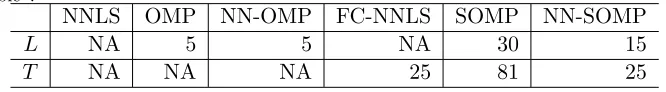
of random training/test splits. For illustration, the optimal parameters

ob-tained by LOOCV of one random training/test split are listed in Table 5.

Note that the NNLS has no parameter to be tuned and hence no training

process is required. For the OMP and NN-OMP, the tuned value of

spar-sity level L is 5; for the FC-NNLS, the tuned value of window size T is 25

(5×5); for the SOMP, the values of L and T are tuned to be 30 and 81

(9×9), respectively; and for the proposed NN-SOMP, the value ofLand T

are tuned to be 15 and 25 (5×5), respectively.

Table 5: Settings of parameters for the Indian Pines dataset in one random training/test split. The values of parameters are determined by LOOCV. “NA” stands for “not appli-cable”.

NNLS OMP NN-OMP FC-NNLS SOMP NN-SOMP

L NA 5 5 NA 30 15

T NA NA NA 25 81 25

6.4.1. Classification performances

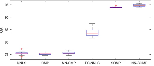
The 10 overall classificationOAs of all six compared methods are recorded

and box-plotted in Figure. 3. For illustration purposes, we also randomly

choose one of the 10 classification results and list the OA, AAand κ

coef-ficient of all methods in Table 6, and depict the classification maps of the

corresponding methods in Figure. 2(e)-2(j), respectively.

From Figure. 3, we can observe two patterns. Firstly, we can observe

that the proposed C-JSM (NN-SOMP) outperforms the other two joint

models, JCM (FC-NNLS) and JSM (SOMP). Also, among the three

sin-gle models, CSM (NN-OMP) performs the best, superior to CM (NNLS)

and SM (OMP). These indicate that incorporating the non-negativity

sparse representation-based classifiers. Secondly, the proposed C-JSM

(NN-SOMP) performs the best among all the compared methods. It indicates

that combining the non-negativity constraints and the joint sparse

repre-sentation can improve the classification performance the most, compared

with the representation with any single constraint, i.e. joint representation,

sparse representation or non-negative representation.

Figure 3: Boxplots of the overall classification accuracies (%) of 3 single models (CM (NNLS), SM (OMP), CSM (NN-OMP)) and 3 joint models (JCM (FC-NNLS), JSM (SOMP), C-JSM (NN-SOMP)) on the Indian Pines dataset.

The one time classification results listed in Table 6 also show that the

proposed C-JSM (NN-SOMP) outperforms other methods, which is aligned

with our findings from the 10 times repeated random splits (Figure. 3). We

also notice two special cases, with class 7 and class 9, that the numbers of

training samples are extremely small, i.e. 3 for class 7 and 2 for class 9,

as listed in Table 4. All methods except for C-JSM (NN-SOMP) do not

perform very well on classifying these two tiny classes of HSI pixels. For

the single models, i.e. CM (NNLS), SM (OMP) and CSM (NN-OMP), the

bad performances may be due to the lack of training samples. For the joint

models of JCM (FC-NNLS) and JSM (SOMP), the performances are even

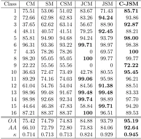
Table 6: The Indian Pines dataset: Ground-truth label and the classification accuracies (%) obtained by CM (NNLS), SM (OMP), CSM (NN-OMP), JCM (FC-NNLS), JSM (SOMP) and C-JSM (NN-SOMP), respectively. The best performance is indicated in bold.

Class CM SM CSM JCM JSM C-JSM

1 75.51 53.06 51.02 83.67 71.43 85.71

2 72.66 62.98 62.83 83.26 94.24 93.86

3 37.65 62.62 63.14 56.67 88.90 92.87

4 48.11 40.57 41.51 79.25 92.45 88.21

5 85.81 94.90 94.68 94.24 93.79 98.00

6 96.31 93.36 93.22 99.71 98.97 98.38

7 4.35 78.26 78.26 0 69.57 100

8 98.20 95.05 95.05 100 99.77 99.77

9 22.22 55.56 55.56 0 0 72.22

10 36.63 72.47 73.49 42.78 80.55 95.45

11 89.29 74.16 74.03 99.06 95.98 96.21

12 61.04 54.76 54.04 84.56 91.38 88.51

13 98.96 99.48 91.67 99.48 99.48 83.33

14 98.98 92.68 92.34 99.74 98.89 97.70

15 44.64 46.38 47.83 58.84 99.71 94.20

16 87.21 88.37 88.37 100 96.51 89.53

OA 75.42 74.79 74.83 84.88 93.79 95.19

AA 66.10 72.79 72.80 73.83 84.06 92.64

are 0. This is because class 7 and class 9 cover narrow regions in the Indian

Pines HSIs (as shown in Figure. 2). The label of the central test pixel can be

dominated by classes adjacent and thus misclassified. However, the proposed

C-JSM (NN-SOMP) relives this spatial-over-smoothness caused by the local

window strategy and outperforms the other five methods with substantial

improvements: achieving 100% against the second best 78.26% for class 7

and achieving 72.22% against the second best 55.56% for class 9.

6.4.2. Effects of parameters

We further investigate the effects of tuning parameters on the

perfor-mance of our proposed C-JSM (NN-SOMP). A sweep of the parameter space

of sparsity levelLand window sizeT is performed during the training phase.

The sparse levelL is tuned from 5 to 80 and the window sizeT ranges from

1 to 289 (17×17). The LOOCV result of C-JSM (NN-SOMP) is depicted

in Figure. 4(a). Within the same parameter space (L and T), we also show

the LOOCV result of JSM (SOMP) in Figure. 4(b) for comparison.

As shown in Figure. 4(a) and Figure. 4(b), we can easily see that the

surface plot ofOAs for C-JSM (NN-SOMP) is much smoother than that of

JSM (SOMP). It implies that C-JSM (NN-SOMP) is more stable than that

of JSM (SOMP) in terms of the performance sensitivity to Land T. More

specifically, we split the 3-D view of theOA surface of C-JSM (NN-SOMP)

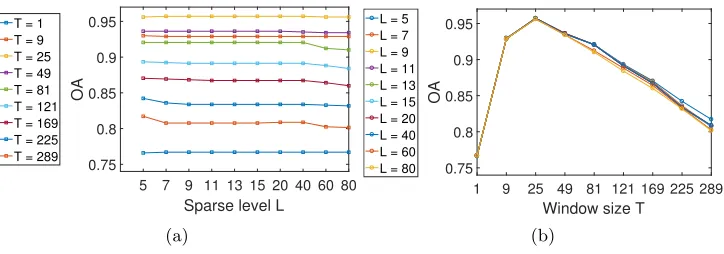
into two 2-D views, which are shown in Figure. 5(a) and Figure. 5(b). It can

be observed that the window size T dominates the performance of C-JSM

whereas the effect of sparsity levelLon the classification performance is not

as sensitive as T.

To further demonstrate the effect of sparsity levelL, we perform

5 0.8 7 9 11 L 13 OA 0.9

15_{20 225}289

169

T

121

40 ₄₉81

60 25 1 9 80 1 (a) 0.8 5 0.9 7 OA 9 1 11 L

1320 169225289

T 121 30406080 1 9 254981

(b)

Figure 4: Overall classification accuracies over window sizeT and sparsity levelLfor (a)

the proposed C-JSM (NN-SOMP) and (b) the JSM (SOMP) on the Indian Pines training dataset via LOOCV.

5 7 9 11 13 15 20 40 60 80

Sparse level L

0.75 0.8 0.85 0.9 0.95 OA

T = 1 T = 9 T = 25 T = 49 T = 81 T = 121 T = 169 T = 225 T = 289

(a)

1 9 25 49 81 121 169 225 289

Window size T 0.75 0.8 0.85 0.9 0.95 OA

L = 5 L = 7 L = 9 L = 11 L = 13 L = 15 L = 20 L = 40 L = 60 L = 80

(b)

Figure 5: Effects of the sparsityLand window sizeT on the performance of the proposed

sizeT to be 25 (5×5) as tuned by LOOCV. This test dataset is the same as

the one used in Table 6 and Figure. 2. We set the level of sparsityLfrom 5

to 80 and depict the obtainedOAs in Figure. 6(a). Accordingly, we record

the real sparsity L0 obtained in different settings of L. Since different test

HSI pixels have different real sparsitiesL0 under a definedL, we record and

box-plot them in Figure. 6(b).

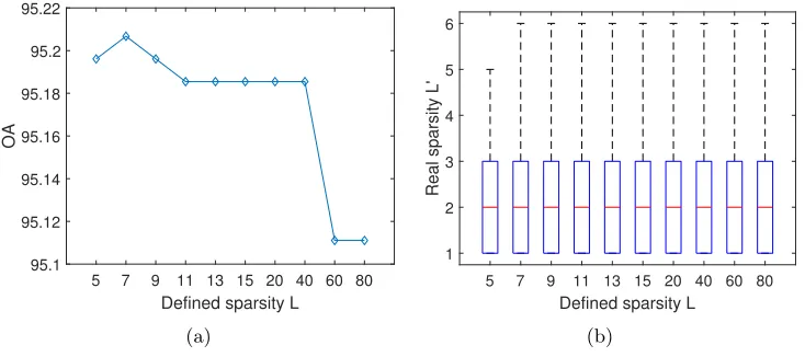
5 7 9 11 13 15 20 40 60 80 Defined sparsity L 95.1

95.12 95.14 95.16 95.18 95.2 95.22

OA

(a)

5 7 9 11 13 15 20 40 60 80

Defined sparsity L

1 2 3 4 5 6

Real sparsity L'

(b)

Figure 6: Window sizeT = 5 on the test dataset of Indian Pines: (a) classification

per-formance (overall accuracies) with sparsity levelL; (b) the real sparsity levelL0obtained

from the test results with sparsity levelL.

It can be seen that, although the best OA occurs at L = 7 when T

is fixed to be 25, the performance only changes slightly with the defined

sparsityL, where the OA changes only from 95.11% to 95.21%. Therefore

the OA = 95.19% of C-JSM (NN-SOMP) listed in Table 6 with L = 5 is

in the range of the stable performance, where the parameters are tuned by

LOOCV and the testing results are reliable.

On the other hand, we can observe that the obtained sparsityL0 ranges

the defined sparsityL are. Furthermore, the obtained maximal sparsity L0

converges to 6 when the defined sparsityLis over 6, as shown in Figure. 6(b).

This explains why the performance of C-JSM (NN-SOMP) is not so sensitive

to the setting of sparsity L. However, the setting of sparsity L still gives

some room for each test HSI pixel to adaptively choose their optimal sparsity

level and hence can achieve a stable and reliable classification performance.

6.4.3. Sparseness and non-negativity

We next demonstrate the effects of sparsity and non-negativity on all the

compared methods by adopting a similar presentation in [50] and depicting

the results in Figures. 7-10. The classification results of all methods are

obtained in parameter settings listed in Table 5. For comparative purposes,

we randomly select two test HSI pixels which belong to class 10 and are

located in (48, 31) and (53, 88): one is correctly classified by all six methods

and the other is only correctly classified by C-JSM (NN-SOMP).

For pixel (48, 31), the associated class-wise residuals obtained by all six

methods are shown in Figure. 7. We can observe that the pixel is correctly

classified by all six methods into class 10, which has the minimum residuals

and is indeed the ground-truth class. Among the six methods, CSM in

Figure. 7(c) and C-JSM in Figure. 7(f), both of which contains both sparse

and non-negative constraints, perform the best with the true class (with the

smallest residual) and the most stable relative to other classes (with all large

residuals).

To investigate further, we plot the obtained coefficients of this pixel in

Figure. 8. Because for the single models (CM, SM and CSM) there is only

one coefficient vector for the test HSI pixelx, there is only one colour shown

1 2 3 4 5 6 7 8 9 10111213141516 Class 0 0.2 0.4 0.6 0.8 1 Normalised residuals (a)

1 2 3 4 5 6 7 8 9 10111213141516 Class 0 0.2 0.4 0.6 0.8 1 Normalised residuals (b)

1 2 3 4 5 6 7 8 9 10111213141516 Class 0 0.2 0.4 0.6 0.8 1 Normalised residuals (c)

1 2 3 4 5 6 7 8 9 10111213141516 Class 0 0.2 0.4 0.6 0.8 1 Normalised residuals (d)

1 2 3 4 5 6 7 8 9 10111213141516 Class 0 0.2 0.4 0.6 0.8 1 Normalised residuals (e)

1 2 3 4 5 6 7 8 9 10111213141516 Class 0 0.2 0.4 0.6 0.8 1 Normalised residuals (f)

Figure 7: Normalised residuals for each class for the pixel located at (48, 31) by (a) CM, (b) SM, (c) CSM, (d) JCM, (e) JSM and (f) C-JSM. The ground-truth label is class 10. The test pixel is correctly identified by all six methods.

0 500 1000 Index of atoms of D 0 0.2 0.4 0.6 0.8 1 Coefficient (a)

0 500 1000

Index of atoms of D -0.5 0 0.5 1 Coefficient (b)

0 500 1000 Index of atoms of D 0 0.2 0.4 0.6 0.8 1 Coefficient (c)

0 500 1000 Index of atoms of D 0 0.2 0.4 0.6 0.8 1 Coefficient (d)

0 500 1000

Index of atoms of D -0.5 0 0.5 1 Coefficient (e)

0 500 1000 Index of atoms of D 0 0.2 0.4 0.6 0.8 1 Coefficient (f)

C-JSM), the label of the central test pixel xc is jointly determined by its

local windowX, hence we plot all the coefficient vectors of the pixels in the

window in different colours. In addition, since the test HSI pixel actually

belongs to class 10, we expect to see that the coefficients mainly lie within

the sub-dictionary of class 10, where the atom indices range from 402 to

490.

From Figure. 8, we can observe that, although all methods can identify

the correct class 10 for pixel (48, 31), the coefficient vectors obtained by

dif-ferent methods are remarkably difdif-ferent, and again, the most neat (sparse)

performances are with C-JSM (Figure. 8(f)) and CSM (Figure. 8(c)). This

also indicates that incorporating the non-negativity constraint into the sparse

model is beneficial, which can produce a more sparse representation.

However, the sparse and non-negative constraints are not the only two

factors that may ensure correct label identification for HSIs. As illustrated

in Figure. 9 and Figure. 10, for a test HSI pixel located in (53, 88), only the

proposed C-JSM identifies its label as class 10 correctly (Figure. 9(f)). In

C-JSM, the non-zero elements of the coefficients vectors of all pixels within

the neighbourhood window mainly lie in class 10 and the label of the central

test pixel is jointly determined by the minimal residuals, which belongs to

class 10 (Figure. 10(f). In contrast, although the coefficient vector obtained

by CSM in Figure. 10(c) is non-negative and most sparse, it lies in class 11,

a wrong class (Figure. 9(c)). This illustrates that the joint representation of

neighbouring pixels on top of the sparsity and non-negativity can positively

contribute to the classification performance for HSIs, and hence the proposed

1 2 3 4 5 6 7 8 9 10111213141516 Class 0 0.2 0.4 0.6 0.8 1 Normalised residuals (a)

1 2 3 4 5 6 7 8 9 10111213141516 Class 0 0.2 0.4 0.6 0.8 1 Normalised residuals (b)

1 2 3 4 5 6 7 8 9 10111213141516 Class 0 0.2 0.4 0.6 0.8 1 Normalised residuals (c)

1 2 3 4 5 6 7 8 9 10111213141516 Class 0 0.2 0.4 0.6 0.8 1 Normalised residuals (d)

1 2 3 4 5 6 7 8 9 10111213141516 Class 0 0.2 0.4 0.6 0.8 1 Normalised residuals (e)

1 2 3 4 5 6 7 8 9 10111213141516 Class 0 0.2 0.4 0.6 0.8 1 Normalised residuals (f)

Figure 9: Normalised residuals for each class for the pixel located at (53, 88) by (a) CM, (b) SM, (c) CSM, (d) JCM, (e) JSM and (f) C-JSM. The ground-truth label is class 10. The test pixel is only correctly identified by our proposed C-JSM.

0 500 1000 Index of atoms of D 0 0.2 0.4 0.6 0.8 1 Coefficient (a)

0 500 1000

Index of atoms of D -0.5 0 0.5 1 Coefficient (b)

0 500 1000 Index of atoms of D 0 0.2 0.4 0.6 0.8 1 Coefficient (c)

0 500 1000 Index of atoms of D 0 0.2 0.4 0.6 0.8 1 Coefficient (d)

0 500 1000

Index of atoms of D -0.5 0 0.5 1 Coefficient (e)

0 500 1000 Index of atoms of D 0 0.2 0.4 0.6 0.8 1 Coefficient (f)

6.5. Real dataset: University of Pavia

The ROSIS University of Pavia dataset consists of 610×340 pixels from

103 spectral bands, with nine ground-truth labels. We randomly choose

only 1% of labelled samples from each class for constructing the

dictio-nary, i.e. D∈_R103×432_{, and use the rest HSI pixels for testing, i.e. X}test _∈

R103×42344. A summary of this dataset is given in Table 7. Again, a false

colour image averaging across all spectral bands, the nine ground-truth

classes, the training set and the test set are shown in Figures. 11(a)-11(d).

Table 7: The Pavia University dataset: Ground-truth labels, class material, the training set and the test set.

Class materials Training Test

1 Asphalt 67 6564

2 Meadows 187 18462

3 Gravel 21 2078

4 Trees 31 3033

5 Painted metal sheets 14 1331

6 Bare soil 51 4978

7 Bitumen 14 1316

8 Self-blocking bricks 37 3645

9 Shadows 10 937

Total 432 42344

For a reliable evaluation, the experiments are also performed by 10 times

random train/test splits, as with the Indian Pines dataset in section 6.4.

For illustration, the optimal values of parameters tuned by LOOCV using

one time train/test random spilt are listed in Table 8. The OAs of all six

compared methods are box-plotted in Figure. 12; we also randomly select one

of 10 classification results and illustrate them in Table 9 and Figure.

11(e)-11(j).

Once again, we can observe that the proposed C-JSM (NN-SOMP)

out-performs other methods. We also note that in Figure. 12 the performance

(a)

1. asphalt 2. meadows 3. gravel 4. trees 5. painted metal sheets 6. bare oil 7. bitumen 8. self-blocking bricks 9. shadows

(b) (c) (d)

(e) (f) (g) (h) (i) (j)

Figure 11: The University of Pavia dataset: (a) mean image shown in the false colour; (b) ground-truth labels; (c) training set (1% pixels randomly chosen); (d) test set.

Clas-sification maps of (e) CM (NNLS),OA= 78.65; (f) SM (OMP),OA = 78.72; (g) CSM

(NN-OMP),OA = 78.75; (h) JCM (FC-NNLS),OA = 82.81; (i) JSM (SOMP),OA =

84.91; (j) C-JSM (NN-SOMP),OA= 86.53.

Table 8: Settings of parameters for the University of Pavia dataset in one random train-ing/test split. The values parameters are determined by LOOCV. “NA” stands for ”not applicable”.

NNLS OMP NN-OMP FC-NNLS SOMP NN-SOMP

L NA 5 5 NA 10 3

NNLS OMP NN-OMP FC-NNLS SOMP NN-SOMP 78

80 82 84 86 88 90

OA

Figure 12: Boxplots of the overall classification accuracies (%) of CM (NNLS), SM (OMP), CSM (NN-OMP), JCM (FC-NNLS), JSM (SOMP) and C-JSM (NN-SOMP) on the Uni-versity of Pavia dataset.

Table 9: The University of Pavia dataset: Ground-truth label and the classification ac-curacies (%) obtained by CM (NNLS), SM (OMP), CSM (NN-OMP), JCM (FC-NNLS), JSM (SOMP) and C-JSM (NN-SOMP), respectively. The best performance is indicated

inbold.

Class CM SM CSM JCM JSM C-JSM

1 85.65 70.75 70.81 98.92 57.46 59.83

2 93.97 92.82 92.82 99.40 98.14 98.55

3 62.70 45.62 45.62 69.30 70.12 77.48

4 87.97 77.28 77.05 93.14 80.25 83.65

5 99.77 99.25 99.25 100.00 100.00 100.00

6 58.00 47.91 47.89 62.82 70.65 80.63

7 42.33 77.43 77.43 28.12 92.63 95.74

8 21.10 74.29 74.29 7.05 93.94 95.34

9 87.41 88.26 89.97 92.74 72.89 31.06

OA 78.65 78.72 78.75 82.81 84.91 86.53

AA 70.99 74.85 75.01 72.39 81.79 80.25

a pattern different from the results shown for the Indian Pines dataset. As

we have analysed in section 6.4.3, sparse and non-negative representations

only may still be insufficient to produce a stable and correct classification.

On the other hand, C-JSM incorporates the sparse and non-negativity

con-straints into the joint modelling of neighbouring pixels, and hence is capable

of providing a more sparse representation and a more stable classification

performance.

6.6. Running time comparison

Table 10: Running time (sec/pixel) spent on testing the Indian Pines dataset, settings of which are shown in Table 4 and Table 5 for 9409 test pixels.

NNLS OMP NN-OMP FC-NNLS SOMP NN-SOMP

Time 0.0058 0.0175 0.0017 0.1195 0.0737 0.0392

We present the time costs for executing the compared algorithms. All

experiments are performed by a Intel i7-3370 CPU using single thread on

the platform of MATLAB R2016b. Table 10 shows the running time of each

method for the Indian Pines dataset. The time is recorded as second per

HSI pixel.

First, we can observe that, among the single models, NN-OMP takes

less time than NNLS and OMP. In fact the obtained coefficients of

NN-OMP are more sparse than the others, as indicated by Figure. 8(a)-8(c) and

Figure. 10(a)-10(c). It implies that the computational burden is lessened

by NN-OMP. Secondly, among the joint models, our proposed NN-SOMP

is more time-efficient than FC-NNLS and SOMP. It is also because the

obtained coefficients from NN-SOMP are more sparse than the others, as

indicated by Figure. 8(d)-8(f) and Figure. 10(d)-10(f), and hence the

6.7. Further remarks

It is worth noting that several literatures have studied the relationship

between the sparsity and non-negativity [42, 51]. It has been shown that the

non-negative least squares (NNLS) may be able to produce sufficient sparse

recovery, without further imposing the sparse regularisations. However, we

remark that this does not imply that the performances of NNLS and the

sparsely regularised NNLS are the same, particular for the classification

problems that are the focus of this paper. That is, the distinct classification

performances of the compared methods of different constraints in this paper

do not conflict the existing findings in [42, 51].

7. Conclusion and future work

To sum up, by considering the non-negativity of coefficients for the

jointly sparse representation of HSI pixels, a new model called cone-based

joint sparse model (J-CSM) has been proposed in this paper. To solve

the C-JSM, a new algorithm, called non-negative simultaneous orthogonal

matching pursuit (NN-SOMP), has also been proposed. The C-JSM

incor-porates the non-negativity of coefficients, as well as the spatial coherence

of the HSI pixels, into one model, yielding a more sparse and stable

rep-resentation for the test HSI pixel whose label is jointly determined by its

neighbouring pixels. As a result, the classification performance of the JSM

is enhanced by the proposed C-JSM.

We notice that the proposed C-JSM may not completely solve the

prob-lems that are caused by the local window scheme. Specifically, the square

shape of the window adopted in this paper indeed introduces bias into the

classifica-tion of the HSI pixel may not have a promising edge-preserving performance.

As aforementioned in the introduction (section 1), several literatures have

studied the improvement of the JSM by adopting size/shape adaptive

win-dows [6–9]. The proposed C-JSM can also be collaboratively conducted

with the window adaptation strategies for enhancing the classification

per-formance. On the other hand, it is also desired to exploit the non-linearity

representation, such as kernelisation [4, 5], of the HSIs together with the

non-negativity constraints for the joint sparse models. These two directions

are our future research on the proposed C-JSM.

Acknowledgment

This work was partially supported by University College London’s

Se-curity Science Doctoral Training Centre under Engineering and Physical

Sciences Research Council (EPSRC) grant EP/G037264/1.

References

[1] J. Wright, Y. Ma, J. Mairal, G. Sapiro, T. S. Huang, S. Yan, Sparse

representation for computer vision and pattern recognition, Proceedings

of the IEEE 98 (6) (2010) 1031–1044.

[2] Y. Han, Y. Yang, Y. Yan, Z. Ma, N. Sebe, X. Zhou, Semisupervised

feature selection via spline regression for video semantic recognition,

IEEE Transactions on Neural Networks and Learning Systems 26 (2)

(2015) 252–264.

[3] Y. Chen, N. M. Nasrabadi, T. D. Tran, Hyperspectral image

classifica-tion using dicclassifica-tionary-based sparse representaclassifica-tion, IEEE Transacclassifica-tions

[4] Y. Chen, N. M. Nasrabadi, T. D. Tran, Hyperspectral image

classifica-tion via kernel sparse representaclassifica-tion, IEEE Transacclassifica-tions on Geoscience

and Remote sensing 51 (1) (2013) 217–231.

[5] J. Liu, Z. Wu, Z. Wei, L. Xiao, L. Sun, Spatial-spectral kernel sparse

representation for hyperspectral image classification, IEEE Journal of

Selected Topics in Applied Earth Observations and Remote Sensing

6 (6) (2013) 2462–2471.

[6] H. Zhang, J. Li, Y. Huang, L. Zhang, A nonlocal weighted joint sparse

representation classification method for hyperspectral imagery, IEEE

Journal of Selected Topics in Applied Earth Observations and Remote

Sensing 7 (6) (2014) 2056–2065.

[7] Y. Y. Tang, H. Yuan, L. Li, Manifold-based sparse representation for

hyperspectral image classification, IEEE Transactions on Geoscience

and Remote Sensing 52 (12) (2014) 7606–7618.

[8] L. Fang, S. Li, X. Kang, J. A. Benediktsson, Spectral–spatial

classifi-cation of hyperspectral images with a superpixel-based discriminative

sparse model, IEEE Transactions on Geoscience and Remote Sensing

53 (8) (2015) 4186–4201.

[9] J. Li, H. Zhang, L. Zhang, Efficient superpixel-level multitask joint

sparse representation for hyperspectral image classification, IEEE

Transactions on Geoscience and Remote Sensing 53 (10) (2015) 5338–

5351.

[10] Y. Zhang, B. Du, L. Zhang, A sparse representation-based binary

Transactions on Geoscience and Remote Sensing 53 (3) (2015) 1346–

1354.

[11] X. Wang, Y. Gao, Y. Cheng, A non-negative sparse semi-supervised

dimensionality reduction algorithm for hyperspectral data,

Neurocom-puting 188 (2016) 275–283.

[12] H. Wang, T. Celik, Sparse representation-based hyperspectral data

pro-cessing: Lossy compression, IEEE Journal of Selected Topics in Applied

Earth Observations and Remote Sensing 10 (5) (2017) 2036–2045.

[13] Y. Zhang, B. Du, L. Zhang, T. Liu, Joint sparse representation and

mul-titask learning for hyperspectral target detection, IEEE Transactions

on Geoscience and Remote Sensing 55 (2) (2017) 894–906.

[14] H. Li, C. Li, C. Zhang, Z. Liu, C. Liu, Hyperspectral image classification

with spatial filtering and l_(2,1) norm, Sensors 17 (2) (2017) 314.

[15] J. A. Tropp, A. C. Gilbert, Signal recovery from random measurements

via orthogonal matching pursuit, IEEE Transactions on Information

Theory 53 (12) (2007) 4655–4666.

[16] A. Soltani-Farani, H. Rabiee, S. Hosseini, Spatial-aware dictionary

learning for hyperspectral image classification, IEEE Transactions on

Geoscience and Remote Sensing 53 (1) (2015) 527–541.

[17] Z. Wang, N. M. Nasrabadi, T. S. Huang, Spatial–spectral

classifica-tion of hyperspectral images using discriminative dicclassifica-tionary designed

by learning vector quantization, IEEE Transactions on Geoscience and

[18] X. Sun, N. M. Nasrabadi, T. D. Tran, Task-driven dictionary

learn-ing for hyperspectral image classification with structured sparsity

con-straints, IEEE Transactions on Geoscience and Remote Sensing 53 (8)

(2015) 4457–4471.

[19] Z. Wang, N. M. Nasrabadi, T. S. Huang, Semisupervised

hyperspec-tral classification using task-driven dictionary learning with Laplacian

regularization, IEEE Transactions on Geoscience and Remote Sensing

53 (3) (2015) 1161–1173.

[20] Z. Wang, J. Liu, J.-H. Xue, Joint sparse model-based discriminative

K-SVD for hyperspectral image classification, Signal Processing 133

(2017) 144–155.

[21] J. A. Tropp, A. C. Gilbert, M. J. Strauss, Algorithms for simultaneous

sparse approximation. part i: Greedy pursuit, Signal Processing 86 (3)

(2006) 572–588.

[22] V. P. Pauca, J. Piper, R. J. Plemmons, Nonnegative matrix

factor-ization for spectral data analysis, Linear Algebra and Its Applications

416 (1) (2006) 29–47.

[23] L. Miao, H. Qi, Endmember extraction from highly mixed data using

minimum volume constrained nonnegative matrix factorization, IEEE

Transactions on Geoscience and Remote Sensing 45 (3) (2007) 765–777.

[24] X. Liu, W. Xia, B. Wang, L. Zhang, An approach based on constrained

nonnegative matrix factorization to unmix hyperspectral data, IEEE

[25] Z. Yang, G. Zhou, S. Xie, S. Ding, J.-M. Yang, J. Zhang, Blind

spec-tral unmixing based on sparse nonnegative matrix factorization, IEEE

Transactions on Image Processing 20 (4) (2011) 1112–1125.

[26] J. Liu, J. Zhang, Y. Gao, C. Zhang, Z. Li, Enhancing spectral unmixing

by local neighborhood weights, IEEE Journal of Selected Topics in

Ap-plied Earth Observations and Remote Sensing 5 (5) (2012) 1545–1552.

[27] N. Wang, B. Du, L. Zhang, An endmember dissimilarity constrained

non-negative matrix factorization method for hyperspectral unmixing,

IEEE Journal of Selected Topics in Applied Earth Observations and

Remote Sensing 6 (2) (2013) 554–569.

[28] X. Lu, H. Wu, Y. Yuan, P. Yan, X. Li, Manifold regularized sparse

NMF for hyperspectral unmixing, IEEE Transactions on Geoscience

and Remote Sensing 51 (5) (2013) 2815–2826.

[29] X. Lu, H. Wu, Y. Yuan, Double constrained NMF for hyperspectral

unmixing, IEEE Transactions on Geoscience and Remote Sensing 52 (5)

(2014) 2746–2758.

[30] C. F´evotte, N. Dobigeon, Nonlinear hyperspectral unmixing with

ro-bust nonnegative matrix factorization, IEEE Transactions on Image

Processing 24 (12) (2015) 4810–4819.

[31] Y. Yuan, M. Fu, X. Lu, Substance dependence constrained sparse NMF

for hyperspectral unmixing, IEEE Transactions on Geoscience and

Re-mote Sensing 53 (6) (2015) 2975–2986.

un-mixing, IEEE Journal of Selected Topics in Applied Earth Observations

and Remote Sensing 8 (6) (2015) 2632–2643.

[33] R. Liu, B. Du, L. Zhang, Hyperspectral unmixing via double abundance

characteristics constraints based NMF, Remote Sensing 8 (6) (2016)

464.

[34] B. Du, S. Wang, N. Wang, L. Zhang, D. Tao, L. Zhang, Hyperspectral

signal unmixing based on constrained non-negative matrix factorization

approach, Neurocomputing 204 (2016) 153–161.

[35] W. He, H. Zhang, L. Zhang, Total variation regularized reweighted

sparse nonnegative matrix factorization for hyperspectral unmixing,

IEEE Transactions on Geoscience and Remote Sensing 55 (7) (2017)

3909–3921.

[36] W. He, H. Zhang, L. Zhang, Sparsity-regularized robust non-negative

matrix factorization for hyperspectral unmixing, IEEE Journal of

Se-lected Topics in Applied Earth Observations and Remote Sensing 9 (9)

(2016) 4267–4279.

[37] W. Dong, F. Fu, G. Shi, X. Cao, J. Wu, G. Li, X. Li, Hyperspectral

im-age super-resolution via non-negative structured sparse representation,

IEEE Transactions on Image Processing 25 (5) (2016) 2337–2352.

[38] Z. Wang, R. Zhu, K. Fukui, J.-H. Xue, Matched shrunken cone detector

(MSCD): Bayesian derivations and case studies for hyperspectral target

detection, IEEE Transactions on Image Processing 26 (11) (2017) 5447–

[39] Z. Wang, Essays on hyperspectral image analysis: classification and

tar-get detection, Ph.D. thesis, University College London (UCL) (2017).

URLhttp://discovery.ucl.ac.uk/id/eprint/1547605

[40] C. Lawson, R. Hanson, Solving Least Squares Problems, Society for

Industrial and Applied Mathematics, 1995.

URLhttp://epubs.siam.org/doi/abs/10.1137/1.9781611971217

[41] R. Bro, S. De Jong, A fast non-negativity-constrained least squares

algorithm, Journal of Chemometrics 11 (5) (1997) 393–401.

[42] A. M. Bruckstein, M. Elad, M. Zibulevsky, On the uniqueness of

non-negative sparse solutions to underdetermined systems of equations,

IEEE Transactions on Information Theory 54 (11) (2008) 4813–4820.

[43] M. Yaghoobi, D. Wu, M. E. Davies, Fast non-negative orthogonal

matching pursuit, IEEE Signal Processing Letters 22 (9) (2015) 1229–

1233.

[44] Q. Shi, B. Du, L. Zhang, Spatial coherence-based batch-mode active

learning for remote sensing image classification, IEEE Transactions on

Image Processing 24 (7) (2015) 2037–2050.

[45] M. H. Van Benthem, M. R. Keenan, Fast algorithm for the solution of

large-scale non-negativity-constrained least squares problems, Journal

of Chemometrics 18 (10) (2004) 441–450.

[46] D. Leviatan, V. N. Temlyakov, Simultaneous approximation by greedy

algorithms, Advances in Computational Mathematics 25 (1-3) (2006)

[47] S. F. Cotter, B. D. Rao, K. Engan, K. Kreutz-Delgado, Sparse solutions

to linear inverse problems with multiple measurement vectors, IEEE

Transactions on Signal Processing 53 (7) (2005) 2477–2488.

[48] P. R. Foundation, A freeware multispectral image data

analy-sis system, _{https://engineering.purdue.edu/~biehl/MultiSpec/}

hyperspectral.html, [Online; accessed 22-July-2014] (2014).

[49] J. A. Richards, X. Jia, Remote Sensing Digital Image Analysis: An

Introduction, New York: Springer-Verlag, 2006.

[50] J. Li, H. Zhang, Y. Huang, L. Zhang, Hyperspectral image

classifica-tion by nonlocal joint collaborative representaclassifica-tion with a locally

adap-tive dictionary, IEEE Transactions on Geoscience and Remote Sensing

52 (6) (2014) 3707–3719.

[51] M. Slawski, M. Hein, Non-negative least squares for high-dimensional

linear models: Consistency and sparse recovery without regularization,