Dynamics of multiplayer games on complex networks using territorial interactions

City, University of London Institutional Repository

Citation

: Schimit, P., Pattni, K. and Broom, M. ORCID: 0000-0002-1698-5495 (2019).

This is the accepted version of the paper.

This version of the publication may differ from the final published

version.

Permanent repository link:

Link to published version

: http://dx.doi.org/10.1103/physreve.99.032306

Copyright and reuse:

City Research Online aims to make research

outputs of City, University of London available to a wider audience.

Copyright and Moral Rights remain with the author(s) and/or copyright

holders. URLs from City Research Online may be freely distributed and

linked to.

Dynamics of multi-player games on complex

networks using territorial interactions

Pedro H. T. Schimit

Informatics and Knowledge Management Graduate Program,

Universidade Nove de Julho, Rua Vergueiro,

235/249, CEP: 01504-000, S˜ao Paulo, SP, Brazil ∗

Karan Pattni

Department of Mathematical Sciences, The University of Liverpool,

Mathematical Sciences Building, Liverpool, L69 7ZL, UK †

Mark Broom

Department of Mathematics, City, University of London,

Northampton Square, London, EC1V 0HB, UK ‡

Abstract

The modelling of evolution in structured populations has been significantly advanced by

evolu-tionary graph theory, which incorporates pairwise relationships between individuals on a network.

More recently, a new framework has been developed to allow for multi-player interactions of

vari-able size in more flexible and potentially changing population structures. While the theory within

this framework has been developed, and simple structures considered, there has been no systematic

consideration of a large range of different population structures, which is the subject of this paper.

We consider a large range of underlying graphical structures for the territorial raider model, the

most commonly used model in the new structure, and consider a variety of important properties of

our structures with the aim of finding factors that determine the fixation probability of mutants.

We find that the graphical temperature and the average group size, as previously defined, are

strong predictors of fixation probability, whilst all other properties considered are poor predictors,

although the clustering coefficient is a useful secondary predictor when combined with either of

temperature or group size. The relationship between temperature/average group size and fixation

probability is sometimes, however, non-monotonic, with a directional reverse occurring around

the temperature associated with what we term “completely mixed” populations in the case of the

Hawk-Dove game, but not the Public Goods game.

Keywords: complex networks, evolution, evolutionary graph theory, game theory, territory.

I. INTRODUCTION

Evolutionary graph theory is an important methodology for considering evolution in a

population with structure, where certain groups of individuals are more likely to interact

than others, for example due to geographical proximity or social status. It considers the

evolution of a population of individuals where each interacts with its neighbours through

a graphical structure, and these interactions affect individual fitness and how the

popu-lation updates, with replacements occurring between neighbouring pairs. The popupopu-lation

structure, i.e. its topology, can strongly affect its evolution [1–7]. Instead of considering

homogeneously structured infinite populations, as is common in evolutionary game theory

[8–10], inhomogeneous populations are considered. Interactions are generally pairwise, using

standard games such as the Prisoner’s Dilemma and the Hawk-Dove game [11–13]. We note

that finite and/or spatial populations have previously been considered in different ways; for

example [14, 15] considered the spatial evolution of cooperative behaviour, [16] considered a

finite population that play a Hawk-Dove game, and [17] considered a Hawk-Dove game on

a lattice.

Evolutionary graph theory generally considers pairwise interactions on a fixed graph

structure between individuals along graph edges, although it is possible to consider

multi-player games through grouping all neighbours of an individual. This nevertheless generally

involves certain groupings of fixed size [18]. For many species, animals either live alone or in

distinct groups on a territory, which can vary considerably in size over time, and often

over-lap with other territories. The same place can thus be used by one, two or many individuals

that will interact and sometimes compete, with the size and composition of the competing

group varying significantly; examples include African wild dogs [19] or roadrunners [20].

Groups can be large cooperative units; for example ant colonies. Primate groups can also

be quite large, including conflicts over dominance and resource division. Such groupings can

be even more complex and varied in human society.

To model such situations, evolutionary games with more than two individuals are needed.

Such multi-player games were introduced by [21] in biological problems and theoretically

expanded by [22] and [23], with more recent modelling work has also been considered in

[24], [25] and [10, Chapter 9]. A multi-player Hawk-Dove game was introduced in [26], and

Thus there is a need for models of evolution on structured populations that incorporate

multiplayer games of varying numbers of players. Broom and Rychtar developed a general

framework for analyzing such multi-player games in structured populations in [26], with

further work on this in [35–38]. In particular, [36] considered evolution using three classical

game scenarios (Hawk-Dove, Prisoner’s Dilemma and fixed fitness) in structured populations

using the Invasion Process dynamics for some simple cases, using the “territorial raider”

model, which used an underlying graphical structure as its basis [39].

In this paper we develop the above work to consider evolution on a large range of complex

networks with a range of structural properties. Complex networks have previously been used

in population evolution by using scale free graphs and lattices [6, 11, 29, 40], random [11]

and regular networks [29, 41]. Although these models consider topological properties of

the mentioned networks, they do not explore a wide range of topological parameters and

structures, which is the focus in this paper. By considering complex network models [42],

we attempt to use topological parameters and different structures to analyze how they are

related to the fixation probability of mutants. Five types of complex network are considered

in this paper: Erd¨os-Renyi (random) network, small-world, scale-free, random ’regular and

Bar´abasi-Albert.

In general throughout the paper we shall use the alternative term “network” in place of

“graph”; they are interchangeable, except that we wish to emphasise that the graphs/networks

that we use represent the population in a way that is distinct to that of a graph in

evolu-tionary graph theory (we shall only use “graph” for the evoluevolu-tionary graph which describes

how the population updates).

We will see throughout the paper that in order to simulate the model in a full range of

different networks and population parameters, we had to run about ten billion different

sim-ulations. An analytical analysis in these circumstances is hard to describe, and a numerical

process had to be formalized to get the results in an acceptable computational time, which

is a critical point in the area [4, 43] for either a large amount of cases or big populations.

In Section II we outline the population model used in this paper, before describing the

computational methodology in Section III and our results in Section IV. We conclude with

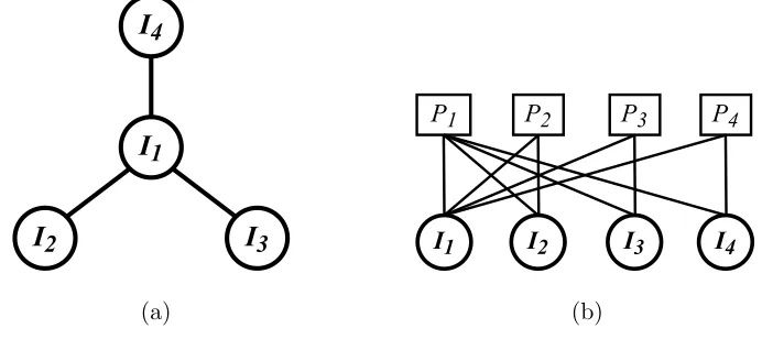
FIG. 1. The fully independent model from [26]. There areN individuals who are distributed over

M places such thatIn visits placePm with probabilitypnm. Individuals interact with one another

when they meet, for example, I1 andI2 can interact with one another when they meet in P1.

II. THE MODELLING FRAMEWORK

The modelling framework is given in full generality in [26]. It incorporates three key

com-ponents; the population structure, the evolutionary dynamics and the evolutionary game. In

particular the general population structure is very flexible. Below we describe an important

special case, which will be the basis of the work in this paper.

A. The fully independent model

A population contains N individuals I1, . . . , IN who are able to move around M places

P1, . . . , PM. The probability of individual Inbeing at placePm is denoted bypnm; see Figure

1 for a visual representation using a bi-partite network. Based on discrete time, at each time

step of the simulation, all individuals move following their given distribution, resulting in the

formation of groups at the different places (the group formed is simply the collection of all

individuals at the given place). Letting G denote any group of individuals, the probability

χ(m,G) that groupG forms in place Pm is given by

χ(m,G) = Y

i∈G

pim

Y

j /∈G

(1−pjm). (1)

will receive a payoff that depends upon the groupGit is present in and the placePm occupied

by this group, denoted by Rn,m,G. IndividualIn’s fitness is then calculated by averaging its

payoffs over all possible groups and places, which is given by

Fn=

X

m

X

G

n∈G

χ(m,G)Rn,m,G. (2)

The fully independent model is still very general, and different examples were introduced

in [26]. Perhaps the most important one of these was the territorial raider model, which was

further developed in [36] and is the basis of the work in this paper.

B. The territorial raider model

In the territorial raider model of [26], a population of N individualsI1, . . . , IN can move

to, and interact at,N different placesP1, . . . , PN, see Figure 2(a). In particular it is assumed

that individualIn lives at place Pn and can also move to neighbouring places, that is,

indi-vidual In has placePn as its original place, returning to it at the end of each iteration. The

population is modelled using a network to represent this scenario, with nodes representing

both individuals and places.

We assume that all individuals make moves which are independent of the moves of others,

and also of the past movements of all individuals (including itself). The probability of an

individual In being at place Pm at any time can thus be denoted by pnm. The networks

that we will study in later sections are thus representations of territorial raider models as

described here, and not the standard graph as in evolutionary graph theory, i.e. they relate

to the general representation as shown in Figure 2(b).

We could allow each individualInto have a distinct movement distribution (pnm)m=1,...,N,

but this would generate (up to)N−1 independent movement parameters for each individual,

and make comparison between different networks difficult. We instead use a natural model

where a single parameterhgoverns every movement, so that an individual withdneighbours

stays at its home node with probabilityh/(h+d) and moves to the node of a given one of its

neighbours with probability 1/(h+d), that is, the individual does not move with probability

h/(h+d) and moves with probability d/(h+d). We term h the home fidelity parameter,

as it is a measure of an individual’s preference for its home node. For high home fidelity,

and there is usually a lot more interaction within the population. Note that choosing h= 1

means that all allowable places, including the home node, are visited with equal probability.

(a) (b)

FIG. 2. (a) Population structure represented using a network where nodes represent individuals

and places. IndividualInlives in place Pnand can visit any neighbouring places. For example, the

home place of I1 is placeP1 but it can visit placesP2, P3 and P4. (b) An alternative visualization

on a bi-partite network where individuals and places are clearly separated.

C. Evolutionary dynamics

An evolutionary graph [1, 44] is a graph with a weighted adjacency matrix W = (wij)

where wij ≥ 0 is the replacement weight, strongly influencing which individuals are more

likely to replace which others. Often weights are right-stochastic, i.e. P

jwij = 1, and this

is the case for the current paper. Every node vn of the evolutionary graph is occupied by

precisely one individual and if wij > 0 then the individual on vi can place a copy of itself

in vj to replace the existing individual. Weights are selected so that the graph is strongly

connected, so there is a route between any pair of nodes.

In this paper, the evolution of the population is described using the Invasion Process[1],

a birth-death process in which the selection happens in the birth event. This process is very

commonly used in evolutionary graph theory, originating in [45], and was adapted to the

modelling framework used here in [36]. In particular, an individual is chosen to give birth

to an offspring with probability

bi =

Fi

PN

n=1Fn

who then replaces one of its neighbours with probability

dij =

wij

PN

k=1wik

. (4)

There are other replacement dynamics that can be considered, for example see [37, 44] for

a list of different evolutionary dynamics that can be used.

We shall define a well-mixed population as one where all replacement weights (except

perhaps the self-replacement weights) take equal value.

The replacement weights used in this paper are based on the assumption that an offspring

of individual Ii is likely to replace another individual Ij proportional to the time Ii and Ij

spend together (note that the offspring of Ii can also replace Ii itself, and the probability

that this happens is proportional to the time Ii is alone). The probability that Ii and Ij

meet is given by summing χ(m,G) over all m such that i, j ∈ G. When they meet, it is

assumed that Ii will spend an equal amount of time with each other individual in group G

and, therefore, we weightχ(m,G) with 1/(|G| −1) since there are |G| −1 other individuals.

Note that this is consistent with the payoffs from our public goods game, as we define in

Section II D, where each pairwise payoff equally contributes to the total payoff an individual

receives. When i =j, we can sum χ(m,G) over all m such that G = {i}. Here there is no

need to weightχ(m,G) becauseIi is alone. The replacement weights are therefore calculated

as follows

wij =

           X m X G i,j∈G

χ(m,G)

|G| −1 i6=j,

X

m

χ(m,{i}) i=j.

(5)

Let S be a state of the population such that n ∈ S implies that node n is occupied by

an individual of type A. There are two absorbing states ∅ in which there are no type A

individuals, and N = {1,2, . . . , N}, where all individuals are of type A. The probability

that a population with initial state S is absorbed in state N is denoted ρA_S, and is referred

to as the fixation probability for state S, most commonly when there is only one type A

individual in S, i.e. S ={i} for i∈ N. The probabilityρA

S is obtained by solving

ρA_S = X

S0_{⊂{1,2,...,N}}

where PSS0 is the probability of transitioning from state S to S0. Since there are N states

with one type A individual in them, the average fixation probability ρA _{is taken which is}

calculated as follows,

ρA= 1

N N

X

i=1

ρA_{i}. (7)

We can similarly define the fixation probability for a type B individual.

The temperature of an individual was defined in [1] to measure how likely an individual

will be replaced in the case of a neutral population where all individuals have constant

fitness. The temperature is defined as follows

Tj =

N

X

i=1,i6=j

wij. (8)

Note that the higher the temperature of an individual, the more likely that that individual

will be replaced. In a homogeneous population structure, like a complete network, each

individual will have the same temperature.

D. Multiplayer games in structured populations

In this section we shall describe three multi-player games, the Public Goods game, the

Hawk-Dove game and the “game” with fixed fitnesses. In each game we will consider a

contests between two different types of individual, A and B, and we will later consider the

fixation probability of a single A in a population ofBs as well as the fixation probability of

a single B in a population ofAs.

1. The multiplayer Hawk-Dove game

A population consists of Hawks, which we label A and Doves, which we label B. All

individuals that meet on a place play a multiplayer Hawk-Dove game, competing for a single

rewardV. If all of these individuals are Doves, they divide the reward equally amongst them.

If there are one or more Hawks, the Doves concede and then all of the Hawks fight, with

the winner getting the reward, while the others receive a costC. In addition, all individuals

Therefore, for a single game involving a group ofa Hawks and b Doves, the average payoffs

for the Hawks and the Doves, respectively, are

R_a,bA =R+V −(a−1)C

a , (9)

R_a,bB =



 

 

R, if a >0,

R+V

b, if a= 0.

(10)

We note that the classical two player Hawk-Dove game is just a special case of our game

as defined. For the two player game for the infinite well-mixed population there is a unique

mixed evolutionarily stable strategy (ESS) ifV < C, and otherwise pure Hawk is the unique

ESS. For a fixed group size n this condition becomes V <(n−1)C, and depends upon the

distribution of the group size when this is variable, as in our case. The parameter values we

have used in this paper (V = 2, C = 1) would thus favour Hawks for the 2-player game, but

not necessariliy for larger groups.

2. The Public Goods game

Here a population consists of Cooperators, A, and Defectors, B. They again start with

a background payoff R, and then play a Public Goods game amongst all of the individuals

on a given place. Following [33], a Cooperator pays a cost C so that other individuals in

the group share the benefit V. We note that we assume that this cost is always paid even

if the Cooperator is alone. Whether this is in fact the case would depend upon the precise

nature of the biological scenario, and it would have been equally plausible to assume that

for lone individuals the cost is not paid. An interesting alternative way of considering lone

individuals was also modelled in [46]. The method that we use is consistent with that used in

[36] and makes the evolution of cooperation harder to achieve than if this was not the case,

and this game is thus a tougher test of when cooperation can evolve than alternatives. We

also note that no similar ambiguity about lone individuals exists for the Hawk-Dove game

above, where the payoff to lone individuals is a natural extension of the contested game.

average payoffs for Cooperators and Defectors of

RA_a,b =



 

 

R−C, a= 1, b= 0,

R−C+ _a+a−_b−1₁V, otherwise,

(11)

RB_a,b =R+ a

a+b−1V. (12)

3. Fixed fitness case

For the fixed fitness game, fitness is frequency-independent and individuals do not really

interact with each other but simply receive a constant payoff depending only upon their

type, independently of the composition of the group. For a group ofa individuals of typeA

and b individuals of type B, we define

RA_a,b=R+V, (13)

RB_a,b=R. (14)

E. Evolutionary graph theory and complex networks

As discussed in Section II B, the territorial raider model that we use is based upon

an underlying network structure, and different network structures can yield very different

results, for example in terms of fixation probability. We shall consider a range of such

networks in this paper, and here we discuss these, together with a few important network

properties.

Erd¨os and R´enyi [47] formulated a random network model, wheren nodes are connected

by e edges randomly chosen among the n(n − 1)/2 possible edges, so that the network

contains a fractionq =e/(n(n−1)/2) of possible edges (this fraction of existing edges is also

called thedensity). Watts and Strogatz [48] proposed a model with similar average shortest

path length to the Erd¨os-R´enyi network (usually small), which can also aggregate nodes

in clusters. Consider a regular network with each node connected to m close individuals,

then rewire a fractionpof the connections. It creates a small-world network, mainly locally

connected with long distance random connections. When p = 1, the network is totally

Such an aggregation of nodes is measured by theclustering coefficient. Consider a nodei

of the network, then the clustering coefficientci for the nodeiis the fraction of existing

con-nections among these neighbors and the total possible, and the average clustering coefficient

is given by ¯c= (1/n)Pn

i=1ci [48].

Some real networks have the property of the rich get richer, that is, nodes that are

introduced into the network are more likely to connect with nodes that have a high number

of connections (the degree of a node). The degree distribution of these networks follows the

expression π(k) ∼ k−γ_{, with γ ' 2.2 [49, 50]. A distribution of nodes π(k) = Ak}−γ_{, with}

A and k constants, is termed scale-free [51] Derived from the scale-free model, Barab´asi

and Albert [52] proposed a different rule: preferential attachment, where the probabilityπba

that a new node will connect to a node i is a proportional to ki, the degree of i, that is,

πba(ki) =ki/

Pn

j=1kj.

III. METHODOLOGY

The networks are representations of territorial raider models. We will consider five models

of undirected networks: Erd¨os-R´enyi, small-world, Barab´asi-Albert, scale-free and regular,

with fixed size of N = 20 nodes. The parameters forming the networks will be varied

accordingly in order to provide the widest topological range within a model. The library

iGraph [53] generates the networks and returns the topological properties.

For the Erd¨os-R´enyi network, the only parameter used as an input is the fraction of

connections. Therefore, mer is varied for the values mer = 0.2,0.205,0.21,0.215, . . . ,1,

generating 161 types of random network. For small-world, the number of close neighbours

connected to each nodemsw and the fraction of rewired connectionspsw are the input

param-eters, and the ranges of each parameter are: msw = 2,4, . . . ,18 and psw = 0.05,0.01, . . . ,1

generating 180 different types of network.

The Barab´asi-Albert networks also have two input parameters: mba is the number of

connections generated per node, and γba the exponent of the probability of a node i with

degree ki being chosen to get an edge πba(ki) = (ki/

Pn

j=1kj)γba according to the

non-linear preferential attachment. When γba = 1 we have the linear and traditional form

of the Barab´asi-Albert model [52]. Therefore, these parameters are varied according to:

The scale-free networks also have the exponent γsf as an input, as well as qsf. The first

is the exponent of the power law distribution π(ki) ∼ k

−γ

i of the network, and the second

is the percentage of total edges to be added to the network. Therefore, we used the values:

qsf = 0.25,0.25,0.3. . . ,1 and γsf = 2,2.25,2.5. . . ,5, generating 208 types of network. In

this case, the configuration model used by iGraph is described in [54].

For regular networks, the only input parameter for generating the network is the degree

of each node, which varies in the interval k= 3,4, . . . ,19, and we have 17 types of network.

Each combination of the three games described in Section II D with two situations per

game (the invasion of a randomly placed individual of each type placed into a population of

the other type) as simulated for each type of network listed previously. Moreover, in order

to have enough variation forh, 50 simulations with randomhwere run for each combination

of games and situations and each type of network, giving 226500 cases. The value of h is

randomly chosen in the interval 0.01 ≤ h ≤ 100 uniformly distributed on the logarithmic

scale.

One simulation is delineated as follows:

• Given the parameters, a network is formed using iGraph;

• The mutant is randomly put on one of the nodes;

• Each individual moves (or not) from its home place according to the model. Every

group with one or more individuals plays the multi-player game;

• Each individual moves (or not) from its home place according to the model. Run

the Birth-Death Process: Randomly pick an individual proportional to its fitness,

and it replaces a random individual from the group it is in; if it is alone, there is no

replacement;

• The simulation ends when either individualsA or B dominate the population.

• This process is run 50000 times to minimise the statistical variability of the results

(95% confidence intervals of estimates always have width (sometimes much) less than

0.01).

Note that we use the typical initial condition called uniform initialization [55], that is,

consis-tency with the previous work [36]. There is also an alternative method called temperature

initialization, see for example [56].

IV. RESULTS

The aim of our analysis is to find good predictors of the key properties of our evolutionary

process, concentrating on the most important, the fixation probability. When dealing with

complex networks, the first objective is often to analyze the dynamical properties of the

system with topological parameters. However, in the model presented, the standard

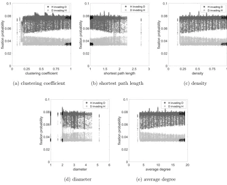
param-eters, including the clustering coefficient, shortest path length, density and diameter, seem

to give very little information about the fixation probability. We can see this in the case of

a. clustering coefficient, b. shortest path length, c. density and d. diameter for all networks

simulations for the Hawk-Dove game in Figure 3. The cases for all networks separately, and

also for the other two games in combination with each of the networks, are similar. However,

as we shall see, the clustering coefficient does have an important secondary role to play.

Note: from here, we will use the original letters of the game’s strategies. For the Public

Goods game, with C for cooperators and D for defectors, and for the Hawk-Dove game, H

for hawks and D for doves.

For small networks [36], we have already seen that the temperature is a good predictor

of the fixation probability. Thus we considered it for this far wider range of (and, with 20

nodes, larger) networks. The temperature is similarly a good predictor over the range of

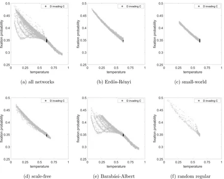
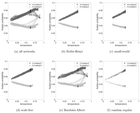
possibilities that we have considered. Figures 4, 5 and 6 show the fixation probability as a

function of temperature for a. all networks, b. Erd¨os-R´enyi, c. small-world, d. scale-free,

e. Barab´asi-Albert and f. random regular networks, for our three games, the public goods

game, hawk-dove game and the fixed fitness case, respectively. Moreover, Figures 7, 8 and

9 show the fixation probability as a function of average group size for the same cases.

In this paper we consider the group size from the individual’s perspective, as opposed to

from the observer’s perspective, see [36] (in [57] these were referred to as the “experienced

group size” and simply the group size, respectively). For example if half of all groups are

of size 2 and half are of size 6, then 3/4 of individuals are in groups of size 6, so the mean

from the individual’s perspective is 5, but from the observer’s perspective is 4).

re-(a) clustering coefficient (b) shortest path length (c) density

(d) diameter (e) average degree

FIG. 3. Fixation probability as a function of a. Clustering coefficient, b. shortest path length, c.

density, d. diameter and e. average degree for all networks simulations for the Hawk-Dove game.

The dark grey dots represent case of H invading D, the light grey dots represent the case of D

invading H and for both cases, black dots represent simulations with well-mixed networks. The

parameter values areR= 10, C= 1, V = 2.

sults. There are many combinations of games and parameters where one of the strategies is

completely dominant for all networks, or where there is no appreciable difference across the

networks, so that the effects are drowned out by the statistical variability due to our

simu-lations. This is in fact a useful observation; for networks generated in the different random

ways that we do, there is often no appreciable difference between fixation probabilities over

exceptional contructed networks, which while of interest lack general applicability.

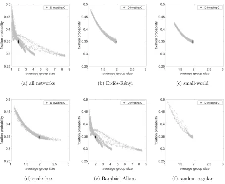
For the Public Goods game we could not find a marked network effect in cases where each

strategy could reasonably invade the other, so a non-flat line could only be found for one

strategy to invade at the expense of the other. Thus in Figures 4 and 7, the probability of C

invading D is small for all networks leading to a flat line close to zero, so we have omitted this

and plotted a range of values on the y-axis to better illustrate the more interesting case of

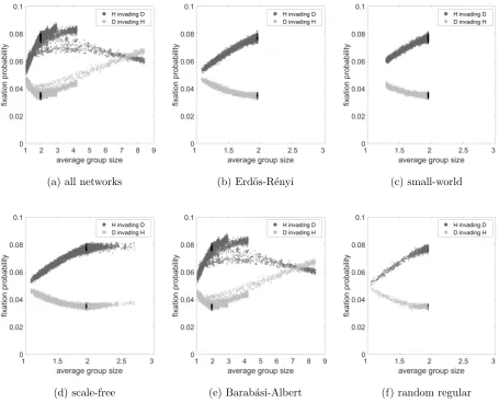
D invading C. For Hawk-Dove games there was interesting behaviour for many parameters,

so we have simply chosen parameters as in [36] in Figures 5 and 8. Finally for the Fixed

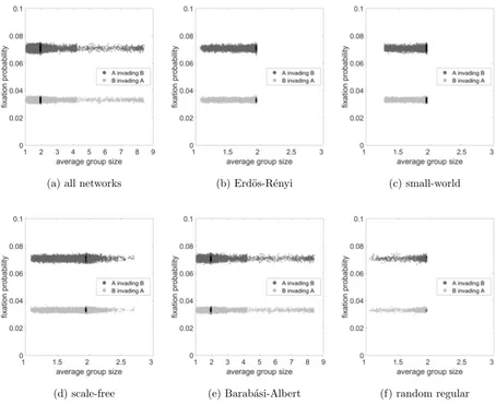
Fitness case there was no interesting behaviour, and we have simply selected parameters

that feature both fixation probabilities clearly on the graph in Figures 6 and 9, but these

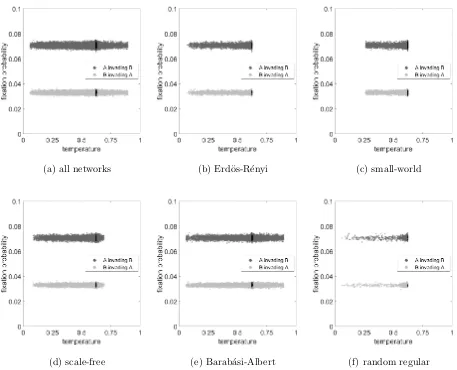
flat lines happened in all cases.

It is worth noting that in Figures 4-9.e, Barab´asi-Albert networks have the wider range

of fixation probability and temperatures values and their curves are thus almost the same

as for the all network data (Figures 4-9.a).

In Figure 4 we see that for the Public Goods game there is a strong linear trend for the

fixation probability in terms of the temperature for all networks, and a straight line fit would

be accurate over the full range for the majority of the networks. However there are some

outlying networks, and the Barab´asi-Albert networks in particular yield some very unusual

behaviour for the lower temperatures. We shall revisit this interesting feature in Section

IV B below.

The Hawk-Dove game in Figure 5 similarly yields nice straight line fits for the fixation

probability in terms of the temperature for all network types except again for Barab´

asi-Albert networks, and to some extent scale-free networks. For Hawks invading a Dove

pop-ulation this is an increasing trend, but for a Dove invading a Hawk poppop-ulation a decreasing

one. For Barab´asi-Albert and scale free networks the trend is reversed at around the

com-pletely mixed temperature, marked by the black dots (see Section IV A) for invading Doves,

and a value somewhat higher than that for the invading Hawks. This is complicated by

the split in the trend in the case of Barab´asi-Albert networks, where a branch breaks off

the main trend in at least two places for both types of individual; we shall investigate this

phenomenon in more detail in Section IV B .

The fixed fitness game simply yields flat lines in Figure 6. There is some between network

(a) all networks (b) Erd¨os-R´enyi (c) small-world

(d) scale-free (e) Barab´asi-Albert (f) random regular

FIG. 4. Fixation probability as a function of temperature considering Public Goods game for a. all

networks, b. Erd¨os-R´enyi, c. small-world, d. scale-free, e. Barab´asi-Albert and f. random regular

networks. For the selected parameters, the fixation probability for C invading D is effectively zero

in all cases, so we have omitted these results. The light grey dots represent the case of D invading

C and the black dots represent simulations with well-mixed networks. The parameter values are

R= 2, C= 1,V = 2.

in predicting these at all.

Figure 7 shows a clear relationship between fixation probability and average group size for

the Public Goods game. Figure 8 shows a similar relationship between fixation probability

and average group size for the Hawk-Dove game. We discuss the interesting issues above in

(a) all networks (b) Erd¨os-R´enyi (c) small-world

(d) scale-free (e) Barab´asi-Albert (f) random regular

FIG. 5. Fixation probability as a function of temperature considering the Hawk-Dove game for

a. all networks, b. Erd¨os-R´enyi, c. small-world, d. scale-free, e. Barab´asi-Albert and f. random

regular networks. The dark grey dots represent case of H invading D, the light grey dots represent

the case of D invading H and for both cases, black dots represent simulations with well-mixed

networks. The parameter values areR= 10, C= 1, V = 2.

general average group size and temperature are strongly correlated, so it is not a surprise to

see a similar relationship here.

Linearity with the temperature can partly be explained by the fact that for the models in

this paper an individual’s temperature effectively reduces to the probability of it not being

alone at the replacement event and in the contests that lead to payoffs (note that these two

(a) all networks (b) Erd¨os-R´enyi (c) small-world

(d) scale-free (e) Barab´asi-Albert (f) random regular

FIG. 6. Fixation probability as a function of temperature considering the fixed fitness game for

a. all networks, b. Erd¨os-R´enyi, c. small-world, d. scale-free, e. Barab´asi-Albert and f. random

regular networks. The dark grey dots represent the case of A invading B, the light grey dots

represent the case of B invading A and for both cases, black dots represent simulations with

well-mixed networks. The parameter values are R= 50,C = 1,V = 2.

subpopulations formed on nodes [37]). Thus for small temperatures, mean temperature is

strongly correlated with the intensity of selection, and the fixation probabilities are close to

straight lines at a temperature of 0. This can be most clearly seen for the Hawk-Dove game,

where lone individuals of both types gain reward V and the intercept with the y-axis is simply

1/N=1/20. This is also true for the public goods game, though here the y-axis intercept is

our chosen parameter values the defectors have twice the fitness of the co-operators, and the

value of (actually marginally above ) 1/2 is that obtained from the classical Moran process.

It is remarkable here, however, that even for quite low temperatures there is quite a variety

in fixation probabilities, i.e. this linear relationship breaks down quite quickly.

(a) all networks (b) Erd¨os-R´enyi (c) small-world

(d) scale-free (e) Barab´asi-Albert (f) random regular

FIG. 7. Fixation probability as a function of average group size considering Public Goods game for

a. all networks, b. Erd¨os-R´enyi, c. small-world, d. scale-free, e. Barab´asi-Albert and f. random

regular networks. The light grey dots represent the case of D invading C and black dots represent

(a) all networks (b) Erd¨os-R´enyi (c) small-world

(d) scale-free (e) Barab´asi-Albert (f) random regular

FIG. 8. Fixation probability as a function of average group size considering the Hawk-Dove game

for a. all networks, b. Erd¨os-R´enyi, c. small-world, d. scale-free, e. Barab´asi-Albert and f. random

regular networks. The dark grey dots represent case of H invading D, the light grey dots represent

the case of D invading H and for both cases, black dots represent simulations with well-mixed

networks. The parameter values areR= 10, C= 1, V = 2.

A. Well-mixed and completely mixed populations

A well-mixed population was previously defined in Section II C as one where all

replace-ment weights (except perhaps the self-replacereplace-ment weights) take equal value. For the

ter-ritorial raider model with movement controlled by the single home fidelity parameter h

(a) all networks (b) Erd¨os-R´enyi (c) small-world

(d) scale-free (e) Barab´asi-Albert (f) random regular

FIG. 9. Fixation probability as a function of average group size considering the fixed fitness game

for a. all networks, b. Erd¨os-R´enyi, c. small-world, d. scale-free, e. Barab´asi-Albert and f. random

regular networks. The dark grey dots represent case of A invading B, the light grey dots represent

the case of B invading A and for both cases, black dots represent simulations with well-mixed

networks. The parameter values areR= 50, C= 1, V = 2.

completely mixed population which occurs when h = 1.

The temperature at a given node, as stated in Section II C, in the territorial raider model

is the probability that that individual is not alone. For a complete network with h = 1,

temperature is simply given by

Tw = 1−

1− 1

n

n−1

≈1−e−1 = 0.632 (15)

(note that the value of the above formula for the case n = 20 used in this paper is Tw =

0.623). Networks with many connections and h not too far from 1 will have temperatures

close to this. We note that here the distribution of the number of an individual’s groupmates

is approximately Poisson (1) and so for example the probability of groups of size 1,2,3 and

4 or more are 0.368, 0.368, 0.184 and 0.080 respectively. Here the mean group size is just 2,

and so larger mean groups will present larger actual group sizes with higher probability.

Erd¨os-R´enyi, small-world and random regular networks have a maximum temperature of

around 0.63, so that the temperatures of completely mixed populations are the maximum

value found. The small average group size is due to the random (and uniform) distribution

of connections which does not concentrate individuals in larger groups. Barab´asi-Albert

networks and scale free networks can reach higher temperatures and higher group sizes than

the other types of network, however. In general more irregular networks combined with low

h can give higher temperatures; for example a star withh= 0 would yield a temperature of

1−1/n, as the central individual would always be alone at another node, whilst all others

would be together in the centre. The black dots in Figures 4 to 9 indicate cases where the

population is close to being completely mixed. We have used randomly generated h values

(and only a few of our networks were complete), so none of the selected networks are exactly

completely mixed. Thus we have marked networks where 0.9≤ h ≤ 1.1 and the density is

higher than 0.9, since these are approximately completely mixed (and as we see, give close

to the above completely mixed fixation probability).

Moreover, Barab´asi-Albert networks and to a small extent scale-free networks have a

change in the temperature trend when the temperature is around 0.63 and average group

size is around 2 in the case of the Hawk Dove game. These values are related to well-mixed

populations and are a threshold between networks of different character, where the higher

temperature networks have connections concentrated on a few nodes and low clustering

B. Unusual network features

In this section we investigate some unusual features of our plots. In particular we consider

two aspects. Firstly, why there is a turning point in the main trend for the Hawk-Dove

game in Figures 5.e and 8.e. Secondly, why on some plots a subset of the networks display

completely different trends to the rest, in particular the two breakaway lines in Figure 5.e

and the set of diverse trends for the low temperature values in Figure 4.e.

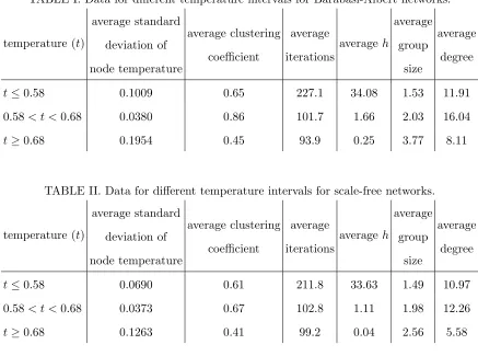
Tables I and II show the average standard deviation of the node temperature, average

clustering coefficient, average iterations (number of iterations for either type of individual

to dominate the population), average h, the average group size and the average degree for

different intervals of temperature for Barab´asi-Albert and scale-free networks, respectively.

The interval 0.58 < t < 0.68 is centered around where the turning point occurs for the

Hawk-Dove game, and the intervalst ≤0.58 and t≥0.68 display two distinct linear trends,

separated by this turning point.

We can see from the tables that the mid-temperature networks have both a higher

clus-tering coefficient and lower standard deviation of the node temperature than for the lower

and higher temperature networks. These mid-temperature networks are generally the best

connected, which naturally leads to a higher clustering coefficient, at least in the types of

net-work that we have considered. These are also the netnet-works closest to the completely mixed

populations, where identical nodes lead to zero standard deviation in the node temperature.

Thus in this range, this standard deviation is low.

We also see that higher temperature is correlated with larger group size. This can help

explain the turning point for the Hawk-Dove game, where Hawks do best (as invader or

invaded population) compared to the other cases. In the cases that we consider Hawks

generally outperform Doves, but for lone inidividuals the payoffs are the same. Thus for low

temperature and so group size Hawk and Dove fixation probabilities are not much different

(each converging to 1/20, since the population size is 20 as temperature converges to 0/ group

size converges to 1). Similarly large groups can involve multiple Hawk-Hawk fights and so

are also bad for Hawks. There is thus an intermediate region where Hawk performance is

relatively at its highest.

Now consider the unusual patterns which depart from a linear trend in the earlier figures,

TABLE I. Data for different temperature intervals for Barab´asi-Albert networks.

temperature (t)

average standard deviation of node temperature average clustering coefficient average iterations average h average group size average degree

t≤0.58 0.1009 0.65 227.1 34.08 1.53 11.91

0.58< t <0.68 0.0380 0.86 101.7 1.66 2.03 16.04

t≥0.68 0.1954 0.45 93.9 0.25 3.77 8.11

TABLE II. Data for different temperature intervals for scale-free networks.

temperature (t)

average standard deviation of node temperature average clustering coefficient average iterations average h average group size average degree

t≤0.58 0.0690 0.61 211.8 33.63 1.49 10.97

0.58< t <0.68 0.0373 0.67 102.8 1.11 1.98 12.26

t≥0.68 0.1263 0.41 99.2 0.04 2.56 5.58

10 we see a colour-coded plot, where four of the key figures from before are repeated, but

this time lighter dots represent higher clustering coefficients. Considering subfigure 10.a

we can clearly see the different lines for low temperature correspond to different values of

clustering coefficent in a very clear way. Higher clustering coefficients give the linear trend

of fixation probability, while low values give the different patterns of low temperatures. The

split into distinct lines here comes about from the way we chose our parameters for the

Barab´asi-Albert model. For instance, the darkest line near low temperatures on Figure 10.a

is related to the number of connections generated per nodemba = 2, and the space between

this trend and the next would be filled if we used mba = 3, since the next trend is related

to mba = 4. We note that for higher temperatures there is less variability in the clustering

coefficients, with all mba cases tending to the same a single trend line here.

Regarding Figures 10.b, 10.c and 10.d, the unusual patterns are always related to low

clustering coefficient values. Comparing these results with Figure 11, we can see that these

points are also related to high values of the standard deviation of the node temperature. Note

(a) Public Goods game, temperature

(b) Hawk-Dove game, temperature

(c) Public Goods game, average group size

(d) Hawk-Dove game, average group size

FIG. 10. Fixation probability as a function of temperature (a. Public Goods game, b. Hawk-Dove

game) and average group size (c. Public Goods game, d. Hawk-Dove game) with a closer look

at the clustering coefficient (see the vertical bar accompanying each figure), with D invading C/D

invading H.

deviation of the node temperature is high. For Figures 10.c, 10.d, 11.c and 11.d, for large

average group size there are a few large groups, which decreases the clustering coefficient

and increases the standard deviation of the node temperature.

(a) Public Goods game, temperature

(b) Hawk-Dove game, temperature

(c) Public Goods game, average group size

(d) Hawk-Dove game, average group size

FIG. 11. Fixation probability as a function of temperature (a. Public Goods game, b. Hawk-Dove

game) and average group size (c. Public Goods game, d. Hawk-Dove game) with a closer look at

the standard deviation of node temperature (see the vertical bar accompanying each figure), with

D invading C/D invading H.

low clustering coefficient are the first to be plotted, and high clustering coefficient are in the

front of the figure. Figure 12 shows a three-dimensional perspective of the same networks,

adding the clustering coefficient in the new axis. Note that the low clustering coefficient

the curves are related to the parameters chosen to form the network. For instance, the curve

with the lowest clustering coefficient is associated with mba= 2, followed by the curve with

mba = 4 and so on.

(a) Public Goods game, temperature

(b) Hawk-Dove game, temperature

(c) Public Goods game, average group size

(d) Hawk-Dove game, average group size

FIG. 12. Three-dimensional figure for the fixation probability as a function of clustering coefficient

and temperature (a. Public Goods game, b. Hawk-Dove game) and average group size (c. Public

Goods game, d. Hawk-Dove game) with a closer look at the standard deviation of node temperature

(see the vertical bar accompanying each figure), with D invading C/D invading H.

Defectors perform better for the cases with a lower clustering coefficient, and so should allow

for better mixing within the population, which is known to favour Defectors. In addition,

as we saw in Tables I and II, a lower clustering coefficient is associated with a higher

standard deviation of node temperature and thus also with a more variable group size, and

we see a consistent effect in Figure 11. The advantage of Defectors over Cooperators in

any given group is the size of the cost C (the only chance for Cooperators to outperform

Defectors being in clustering preferentially with other Cooperators), but the total payoff is

smaller, and so the relative advantage larger, for lone individuals, with any group size above

1 which involves a cooperator being approximately equivalent. Thus Defectors have the

largest fixation probability when the probability of individuals being alone is largest, which

occurs when the group size is most variable. More variable group sizes are similarly bad

for Hawks as we have discussed above, so there is a similar effect here with lower clustering

coefficients favouring Doves. For a fixed temperature group size increases with a decreasing

clustering coefficient. Thus for a fixed temperature, a lower clustering coefficient again

favours Doves as we see in Figure 10.a. However, for Defectors, this effect is reversed with a

higher clustering coefficient favouring Defectors, since the smaller group sizes means there

is a greater probability of being a lone individual.

In summary, the Barab´asi-Albert model is the only one to allow temperatures significantly

higher than those found in well-mixed populations, considering the size of the network used

in this paper. The preferential attachment rule of the model allows the network to have

a small number of highly connected nodes, which return a higher average group size. The

networks with few connections have low clustering coefficient and the widest temperature

range. Small groups favour Hawks invading Doves and Defectors invading Cooperators

(the small groups should be bigger than one to favour the Hawks). Since Barab´asi-Albert

networks allow large groups, it favours Doves invading Hawks and decreases the fixation

probability for Defectors invading Cooperators.

V. DISCUSSION

In this paper, we have built upon the existing framework of Broom and Rycht´aˇr [26],

in particular investigating factors that determine the fixation probability of mutants

model is built on an underlying network structure, and we used five types of complex

net-works: Erd¨os-Renyi (random), small-world, scale-free, Bar´abasi-Albert and random regular

networks. We also considered a number of population properties in conjunction with these

networks; these were five topological parameters of the generated networks: average degree,

clustering coefficient, shortest path, density and diameter, together with the graphical

tem-perature (using the replacement weight matrix), the mean group size and the model’s “home

fidelity” parameter.

The main objective of the paper was to find population properties which could predict

the fixation probability. The topological parameters were poor predictors, and out of the

other factors, the graphical temperature was the best predictor, as also found in previous

work on very small networks [36], and average group size was also a strong predictor. In

addition, the clustering coefficient proved to a useful secondary predictor, in conjunction

with the others.

The predictions of our model are often in accord with those from classical evolutionary

graph theory. Populations structured over star networks tend to favour Doves invading

Hawks due to large groups [45], and we also have this effect for small networks [36]. In

[29], the wealth distribution model using Public-Goods game found that stars increase the

inequality in the population due to a better situation for Defectors. In [11], scale-free

net-works were the hottest network in the paper, and the hottest cases were where the Doves

performed better. We note that the linear relationship with mean temperature is new;

typi-cally evolutionary graph theory models exclude self-weights, and then the mean temperature

is just 1 for all graphs (for some consequences of including self-weights in evolutionary graph

theory, see [58]). A similar relationship with a differently defined temperature can be seen

in [59] for a model of a finite well-mixed population.

This similarity of predictions is not surprising, as both models are built on sensible

assumptions which are realistic for non-extreme situations (e.g. graphs that are close to

being well-mixed). There are some phenomena that we have observed in our model that

have not been observed for evolutionary graph theory, however, in particular the results from

section IV B where we discuss unusual features of our plots, including the turning point in

the graphs with high temperatures and the plots where for some temperatures there are

multiple trend lines associated with different clustering coefficients. These features occur for

group sizes, and it is in such graphs where the assumptions of our model and those of classical

evolutionary graph theory differ most. When large groups can form, the non-linearity of our

model and the payoffs of the constituent games are most in evidence.

In general, an important feature of our model is the existence of variable group sizes,

which is a realistic feature absent from evolutionary graph theory models. The fact that

evolutionary graph theory and our more involved framework often yield similar results can be

argued as a case of the simpler model being sufficient to make good predictions in a range

of circumstances, just as well-mixed populations from classical evolutionary game theory

give results close to evolutionary graph theory in general, and only when the structural

component is significant do the advantages of the evolutionary graph theory methodology

become apparent. In the same way, it is when structure would yield significantly variable

group sizes, and in particular large groups, that evolutionary graph theory models do not

produce the predictions that our methodology does.

The variability of group sizes includes the possibility of being alone. Thus how we define

the payoff for being alone can have a significant effect, especially when mean group sizes

are small, as we have mentioned in Section II D 2. We note that it would be possible to

consider lone individuals in evolutionary graph theory too by introducing self-loops within

the graph, and the likelihood of individual interactions could be decided by choosing an

appropriate weight to this link. The public goods game considered also has a maximum

payoff of V, irrespective of how many cooperators there are. Alternative games could thus

yield a stronger effect of group size overall. We note that there are many different multiplayer

games that we could use, including different types of public goods games, and we consider

these, and the effect of different mean group sizes, in the paper [60]. In fact the discussion

about the effect of individuals being alone can in one sense be seen as a strength of our

work. Lone individuals arise naturally as part of our framework, and we would argue that

this important feature has often been lost due to the imposition of pairwise models for all

interactions.

An interesting feature of our results is that for the public goods game, the fixation

probability of defectors has a decreasing trend with the average group size. At first sight

this contradicts earlier work where the defectors’ fixation probability increased with the

group size as in [37] or [33]. A key difference here is that in the above work the group sizes

very variable group sizes, with a significant probability of lone individuals. This particularly

affects the initial trend for small mean group sizes as defectors do well for lone individuals,

and cooperators do especially well for actual (as opposed to mean) group size two (again see

[37]). We can see from the figures 7.d and 7.e that the trend is initially steep but flattens

down. In our version of the public goods game, lone cooperators still pay a cost. We have

checked an alternative version of the game where they do not (figure not shown). In that

version, the trend is reverted, and we observe a clear increase in the fixation probability

with the mean group size, for all group sizes.

The existence of lone individuals is not completely the answer, as the trend does keep

decreasing even for quite large group sizes. The variability of the group sizes itself is an

important factor here. A common (but definitely not universal) feature of variable group

sizes (see [60], which considered a range of multi-player games) is that the more variable the

group size, the better the cooperators perform relative to the defectors (in particular the

larger the incentive function, the larger the payoff to a cooperator minus that to a defector).

As group sizes go up for our model both mean and variance increase, so that these effects

pull in opposite directions. In general specific choice of game, underlying graph, dynamics

and variability of group size will all have an effect on this issue.

Although the temperature (and to a lesser extent group size) is a good predictor of the

fixation probability, an interesting result is the non-monotonic trend found on scale-free and

Bar´abasi-Albert networks for the Hawk-Dove game. Moreover, the temperature has values

higher than for the completely mixed case only for these networks, and the turning point in

the trend happened at around the completely mixed temperature of 0.632. For these cases,

consideration of the clustering coefficient helped us to understand that the concentration of

connections to a small number of nodes enables “hotter” networks that suppresses selection.

In particular, when the clustering coefficient is low, there could be a marked deviated from

the trend as observed in the figures.

Moreover, the proposed numerical methodology is an alternative to deal efficiently with

large networks. The system of linear equations grows exponentially with the number of nodes

[36, 61] and considering the large number of different networks treated here, an analytical

resolution would be arduous. The methodology used here can be applied to consider models

from the framework of [26] even for much larger populations. Therefore, this framework can

There are a number of promising directions for future work. In previous work, especially

[36], we have only considered this model for relatively small networks, and whilst our results

are consistent with theirs, consideration of many larger networks have enabled a clearer

pattern, and also unusual features, to emerge. In future work we will explore these various

patterns in more detail, and also consider the effect of different dynamics on the fixation

probability. We can apply the methodology for larger networks as described above. Although

the simulations for 20 nodes took about 1100 hours to complete in a PC with 4.4GHz and

16Gb RAM, increasing the size of the network would result in a wider range of parameters,

and it would be interesting to see if the trend change found for scale-free networks would

be similar to the Bar´abasi-Albert case. We use a infrastructure for parallel computation,

which reduced the simulation time by approximately 70%.

Can we combine the existing predictors, temperature, mean group size and clustering

co-efficient to provide a more effective single predictor? Can we find other additional secondary

predictors, that in combination with the existing predictors, especially the temperature,

pro-vide even more effective predictors?

There are a number of different evolutionary dynamics that can be applied, as detailed

in [37], and it is important to see what predictive factors are needed for these alternative

dynamics; for example, will a different type of temperature be needed in some cases? It is

known that different dynamics can have a big effect in evolutionary graph theory, and that

is also true in this framework, as seen in [37].

Predicting network properties is a relevant problem in different areas. In evolutionary

graph theory, the graph structures that promote the evolution of cooperation have been

extensively analysed, for instance, using direct reciprocity on graphs [62] and directed

net-works [63]. Recently, [64] considered linking together structures that are unpromising for

cooperation to produce an overall structure that favours it; this is a similar effect to that

from our more extreme Barab´asi-Albert networks which generate a small number of

sepa-rate clusters. Related problems consider the evolution of social behaviour [65] and spatial

ACKNOWLEDGMENTS

PHTS is supported by grants #303743/2016-6 and #402874/2016-1 of Conselho Nacional

de Desenvolvimento Cient´ıfico e Tecnol´ogico (CNPq) and grant #2017/12671-8, S˜ao Paulo

Research Foundation (FAPESP).

This work was supported by funding from the European Union’s Horizon 2020 research and

innovation programme under the Marie Sklodowska-Curie grant agreement No 690817 (MB).

KP is funded by EPSRC grant reference EP/N014499/1.

[1] E. Lieberman, C. Hauert, and M. Nowak, Nature 433, 312 (2005).

[2] T. Antal and I. Scheuring, Bulletin of Mathematical Biology 68, 1923 (2006).

[3] M. Nowak, Evolutionary Dynamics, Exploring the Equations of Life (Harward University

Press, Cambridge, Mass., 2006).

[4] M. Broom and J. Rycht´aˇr, Proceedings of the Royal Society A: Mathematical, Physical and

Engineering Science 464, 2609 (2008).

[5] B. Voorhees and A. Murray, Proceedings of the Royal Society A: Mathematical, Physical and

Engineering Science 469 (2013), 10.1098/rspa.2012.0676.

[6] W. Maciejewski, F. Fu, and C. Hauert, PLoS Computational Biology10(2014),

10.1371/jour-nal.pcbi.1003567, arXiv:arXiv:1312.2942v1.

[7] L. M. Ying, J. Zhou, M. Tang, S. G. Guan, and Y. Zou, Frontiers of Physics 13(2018).

[8] J. Maynard Smith,Evolution and the Theory of Games (Cambridge University Press, 1982).

[9] J. Hofbauer and K. Sigmund,Evolutionary games and population dynamics (Cambridge

Uni-versity Press, 1998).

[10] M. Broom and J. Rycht´aˇr,Game-Theoretical Models in Biology (CRC Press, Boca Raton, FL,

2013).

[11] H. Ohtsuki, C. Hauert, E. Lieberman, and M. A. Nowak, Nature 441, 502 (2006),

arXiv:NIHMS150003.

[12] F. Santos and J. Pacheco, Journal of Evolutionary Biology 19, 726 (2006).

[13] C. Hadjichrysanthou, M. Broom, and J. Rycht´aˇr, Dynamic Games and Applications 1, 386

[14] M. Nowak and R. May, Nature359, 826 (1992).

[15] M. Nowak and R. May, International Journal of Bifurcation and Chaos 3, 35 (1993).

[16] M. Schaffer, Journal of Theoretical Biology 132, 469 (1988).

[17] T. Killingback and M. Doebeli, Proceedings of the Royal Society of London. Series B: Biological

Sciences 263, 1135 (1996).

[18] A. Li, B. Wu, and L. Wang, Scientific Reports4 (2014).

[19] J. Ginsberg and D. Macdonald, Foxes, wolves, jackals, and dogs: an action plan for the

conservation of canids (IUNC, Gland, Switzerland, 1990).

[20] S. Kelley, D. Ransom Jr, J. Butcher, G. Schulz, B. Surber, W. Pinchak, C. Santamaria, and

L. Hurtado, Journal of Field Ornithology 82, 165 (2011).

[21] G. Palm, Journal of Mathematical Biology 19, 329 (1984).

[22] M. Broom, C. Cannings, and G. Vickers, Bulletin of Mathematical Biology 59, 931 (1997).

[23] M. Bukowski and J. Miekisz, International Journal of Game Theory 33, 41 (2004).

[24] C. Gokhale and A. Traulsen, Proceedings of the National Academy of Sciences 107, 5500

(2010).

[25] C. Gokhale and A. Traulsen, Dynamic Games and Applications , 1 (2014).

[26] M. Broom and J. Rycht´aˇr, Journal of Theoretical Biology 302, 70 (2012).

[27] C. Hauert, S. De Monte, J. Hofbauer, and K. Sigmund, Science296, 1129 (2002).

[28] M. Milinski, D. Semmann, H. Krambeck, and J. Marotzke, Proceedings of the National

Academy of Sciences of the United States of America 103, 3994 (2006).

[29] F. C. Santos, M. D. Santos, and J. M. Pacheco, Nature454, 213 (2008), NIHMS150003.

[30] S. Kurokawa and Y. Ihara, Proceedings of the Royal Society B: Biological Sciences276, 1379

(2009).

[31] M. Souza, J. Pacheco, and F. Santos, Journal of Theoretical Biology 260, 581 (2009).

[32] F. Santos and J. Pacheco, Proceedings of the National Academy of Sciences108, 10421 (2011).

[33] M. van Veelen and M. Nowak, Journal of Theoretical Biology 292, 116 (2012).

[34] S. Kurokawa and Y. Ihara, Theoretical Population Biology 84, 1 (2013).

[35] M. Bruni, M. Broom, and J. Rycht´aˇr, Involve, a Journal of Mathematics 7, 129 (2014).

[36] M. Broom, C. Lafaye, K. Pattni, and J. Rycht´aˇr, Journal of Mathematical Biology 71, 1551

(2015).

[38] K. Pattni, M. Broom, and J. Rycht´aˇr, Discrete & Continuous Dynamical Systems - B 23,

1975 (2017).

[39] N. Galanter, D. Silva, J. T. Rowell, and J. Rycht´aˇr, Journal of Theoretical Biology412, 100

(2017).

[40] F. D´ebarre, C. Hauert, and M. Doebeli, Nature Communications5, 3409 (2014).

[41] A. McAvoy and C. Hauert, Journal of the Royal Society, Interface / the Royal Society 12,

20150420 (2015).

[42] S. Boccaletti, V. Latora, Y. Moreno, M. Chavez, and D. U. Hwang, Physics Reports 424,

175 (2006).

[43] L. Hindersin, M. M¨oller, A. Traulsen, and B. Bauer, BioSystems 150, 87 (2016), 1511.02696.

[44] K. Pattni, M. Broom, J. Rycht´aˇr, and L. J. Silvers, Proceedings of the Royal Society of London

A: Mathematical, Physical and Engineering Sciences 471 (2015), 10.1098/rspa.2015.0334.

[45] H. Lieberman and M. A. Nowak, Nature 1, 1 (2005).

[46] C. Hauert and G. Szab´o, Complexity 8, 31 (2003).

[47] P. Erdos and A. R´enyi, I. Publicationes Mathematicae6, 290 (1959).

[48] D. Watts and S. Strogatz, Nature393, 440 (1998).

[49] R. Albert and A. L. Barabasi, Reviews of Modern Physics74, 47 (2002).

[50] M. Newman,Networks: An Introduction(Oxford University Press, Inc., New York, NY, USA,

2010).

[51] B. Bollob´as, O. Riordan, J. Spencer, and G. Tusndy, Random Structures & Algorithms 18,

279 (2001).

[52] A.-L. Barab´asi and R. Albert, Science 286, 509 (1999).

[53] G. Csardi and T. Nepusz, InterJournal, Complex Systems , 1695 (2006).

[54] K.-I. Goh, B. Kahng, and D. Kim, Phys. Rev. Lett. 87, 278701 (2001).

[55] B. Adlam, K. Chatterjee, and M. A. Nowak, Proceedings of the Royal Society of London

A: Mathematical, Physical and Engineering Sciences 471 (2015), 10.1098/rspa.2015.0114,

http://rspa.royalsocietypublishing.org/content/471/2181/20150114.full.pdf.

[56] B. Allen, A. Traulsen, C. Tarnita, and M. Nowak, Journal of Theoretical Biology 299, 97

(2012).

[57] J. Pe˜na and G. N¨oldeke, Journal of Theoretical Biology 389, 72 (2016).

Mathematical, Physical and Engineering Sciences, Vol. 471 (2015).

[59] A. Traulsen, M. A. Nowak, and J. M. Pacheco, Journal of Theoretical Biology 244, 349

(2007).

[60] M. Broom, K. Pattni, and J. Rycht´aˇr, Bulletin of Mathematical Biology , 1 (2018).

[61] M. Broom, C. Hadjichrysanthou, and J. Rycht´aˇr, Proceedings of the Royal Society A:

Math-ematical, Physical and Engineering Science 466(2010), 10.1098/rspa.2009.0487.

[62] H. Ohtsuki and M. A. Nowak, Journal of Theoretical Biology 247, 462 (2007).

[63] N. Masuda and H. Ohtsuki, New Journal of Physics11(2009).

[64] B. Fotouhi, N. Momeni, B. Allen, and M. A. Nowak, Nature Human Behaviour2, 492 (2018).

[65] S. Kurokawa and Y. Ihara, Theoretical Population Biology 84, 1 (2013).

[66] B. Allen, J. Gore, and M. A. Nowak, Elife 2, e01169 (2013).

[67] J. Pe˜na, G. N¨oldeke, and L. Lehmann, Journal of Theoretical Biology 382, 122 (2015).